| Issue |
A&A
Volume 687, July 2024
|
|
|---|---|---|
| Article Number | A185 | |
| Number of page(s) | 13 | |
| Section | Astrophysical processes | |
| DOI | https://doi.org/10.1051/0004-6361/202349134 | |
| Published online | 09 July 2024 | |
Black hole outflows initiated by a large-scale magnetic field
Effects of aligned and misaligned spin
1
Center for Theoretical Physics, Polish Academy of Sciences, Al. Lotników 32/46, 02-668 Warsaw, Polandbestin@cft.edu.pl
e-mail: bestin@cft.edu.pl
2
Astronomical Institute, Czech Academy of Sciences, Boční II, 141 00 Prague, Czech Republic
Received:
30
December
2023
Accepted:
23
March
2024
Context. Accreting black hole sources show variable outflows at different mass scales. For instance, in the case of galactic nuclei, our own Galactic center Sgr A* exhibits flares and outbursts in the X-ray and infrared bands. Recent studies suggest that the inner magnetospheres of these sources have a pronounced effect on these emissions.
Aims. Accreting plasma carries the frozen-in magnetic flux along with it down to the black hole horizon. During the infall, the magnetic field intensifies, and this can lead to a magnetically arrested state. We investigate the competing effects of inflows at the black hole horizon and the outflows that develop in the accreting plasma through the action of the magnetic field in the inner magnetosphere, and we determine the implications of these effects.
Methods. We started with a spherically symmetric Bondi-type inflow and introduced a magnetic field. In order to understand the influence of the initial configuration, we started the computations with an aligned magnetic field with respect to the rotation axis of the black hole. Then we proceeded to the case of magnetic fields that are inclined to the rotation axis of the black hole. We employed the 2D and 3D versions of the code HARM for the aligned field models and used the 3D version for the inclined field. We compared the results of computations with each other.
Results. We observe that the magnetic lines of force start to accrete with the plasma while an equatorial intermittent outflow develops. This outflow continues to push some material away from the black hole in the equatorial plane, while some other material is ejected in the vertical direction from the plane. In consequence, the accretion rate fluctuates as well. The direction of the black hole spin prevails at later stages. It determines the flow geometry near the event horizon. On larger scales, however, the flow geometry remains influenced by the initial inclination of the field.
Key words: accretion / accretion disks / black hole physics / magnetic fields / magnetohydrodynamics (MHD) / relativistic processes
© The Authors 2024
 Open Access article, published by EDP Sciences, under the terms of the Creative Commons Attribution License (https://creativecommons.org/licenses/by/4.0), which permits unrestricted use, distribution, and reproduction in any medium, provided the original work is properly cited.
This article is published in open access under the Subscribe to Open model. Subscribe to A&A to support open access publication.
1. Introduction
Various observational studies indicate that an accreting black hole acts as an engine that powers high-energy phenomena in jets from active galactic nuclei (AGN), including gamma-ray bursts (e.g., Dermer & Menon 2009; Meier 2012). Black holes attract the gaseous material from their surrounding environment (Rees & Volonteri 2006). The accretion of plasma onto the central compact object by its gravitational force produces various observable effects, including relativistic jets and outflows in the form of winds (in particular in stellar mass black holes; see Narayan & McClintock 2015; Fender & Gallo 2014). It is appropriate to assume that plasma at large scales is magnetized due to its environment. As the accretion proceeds, a strong magnetic pressure can develop near the black hole horizon and can act against accretion itself. This sometimes leads to the formation of a magnetically arrested disk (MAD; Narayan et al. 2003; Tchekhovskoy et al. 2011; Event Horizon Telescope Collaboration 2021). The accumulated magnetic flux can inhibit further accretion, and this plays a role in the formation of the relativistic jets that are observed from the black hole sources.
A mechanism that supports the formation and collimation of jets from a Kerr black hole surrounded by magnetic field was originally described by Blandford & Znajek (1977). According to this mechanism, the jet can extract energy from the rotation of the black hole, which was later demonstrated in general relativistic magnetohydrodynamic (GRMHD) simulations (Tchekhovskoy et al. 2011). On the other hand, in the case of rapidly spinning black holes, Meissner-like expulsion of magnetic field lines is expected, which can adversely affect the efficiency of the Blandford-Znajek mechanism (Bičák & Janiš 1985; King et al. 1975). It was later shown by Komissarov & McKinney (2007) and others that this effect is diminished by the inward force of accretion, and the Blandford-Znajek mechanism is often sustained. The black hole does not hold the magnetic field by itself. When the accretion rate begins to diminish, the magnetic field lines can push the clumps of plasma away from the black hole. The magnetically inhibited inflow can eventually transform into an outflow above and below the disk, where the current sheet forms (Ripperda et al. 2020, 2022).
While the occurrence of the magnetically arrested state is frequently observed in GRMHD simulations of accreting black holes, the development of the system is rather sensitive to the conditions at the outer boundary, to the dimensionality of the computation, and to other assumptions about the flow. El Mellah et al. (2022, 2023) revealed a separatrix and current sheet in a centrifugally determined flow where particles can be accelerated along a characteristic inclination angle, which is also seen in the synchrotron emission when the computation includes the associated radiation losses. In the latter paper, the authors presented global 3D general relativistic particle-in-cell (PIC) simulations of a black hole magnetosphere with the aim to replicate the observed hot spots and flares around Sgr A*. Their simulations revealed the formation of magnetic flux ropes and the subsequent dissipation of electromagnetic energy through magnetic reconnection. Furthermore, they showed that the synchrotron emission from these flux ropes can reproduce the observed flares, and that the hot spot motion and duration are consistent with the model predictions. Their study also offered constraints on the spin of Sgr A* through the study of the dynamics magnetosphere. Chashkina et al. (2021) presented a series of numerical simulations in which the outflows were activated from the black hole due to the advection of small-scale magnetic fields. They used small-scale magnetic field loops, and these configurations are shown to potentially support the formation of quasi-striped Blandford-Znajek jets. Their configuration also seemed to lead to enhanced dissipation and to the generation of plasmoids in current sheets that formed in the vicinity of the black horizon. This might act as a mechanism that powers hard X-ray emission in many accreting black hole systems.
Crinquand et al. (2022) identified a persistent equatorial current sheet and some flaring activity in a setup relevant for a very low accretion state (see also Hakobyan et al. 2023). Further, Kwan et al. (2023) explored Bondi-type accretion, and they demonstrated that even in this system, the flow can be magnetically arrested and can produce episodic jets that are launched predominantly along the common rotation axis of the black hole and the accretion disk. They demonstrated that the magnitude of the initial specific angular momentum of the gas plays a vital role in the formation of a MAD state and in the subsequent launching of powerful jets. They also noted that for a very powerful and stable relativistic jet, the accretion flow has to sustain a MAD state that requires a nonzero value of the specific angular momentum for the gas, even though this threshold value is very low (it corresponds to a circularization radius between 10rg and 50rg).
Ressler et al. (2021) also explored zero angular momentum accretion onto a rapidly rotating black hole and found that the jet power peaks for an initially tilted magnetic field with respect to the black hole spin axis as this geometry maximizes the magnetic flux across the event horizon. They assumed a uniform magnetic field with different tilt angles, with a uniform initial plasma β of 100 and a high value of the black hole spin (a = 0.9375). In this setup, they noted that polar jets developed almost regardless of the magnetic tilt angles, driven by a nearly magnetically arrested configuration in the equatorial region of the flow. Recently, Ressler et al. (2023) performed realistic 3D GRMHD model computations in the context of wind-fed accretion from a set of Wolf-Rayet stars near the Sgr A* supermassive black hole. They observed a stochastic behavior of the system, with a jet that changed its direction with respect to the black hole rotation axis, and the MAD state was temporarily suppressed during quiescent periods.
Curd & Narayan (2023) investigated the MAD state with their GRRMHD simulations. Their models resulted in relativistic jets. Their models showed significant variability in the outgoing radiation, which they attributed to episodes of magnetic flux eruptions. Suková et al. (2023) explored the possibility that jetted outflows might be assisted by repetitive triggering by orbiting perturbers, such as an intermediate secondary black hole.
In this work, we focus on the structure and rate of plasma outflows mediated by the presence of large-scale magnetic fields (e.g., Wald 1974) and the resultant evolution of the plasma and the frozen-in magnetic field in the vicinity of the black hole horizon. We examine the competing effects of mass inflows and outflows driven by a large-scale asymptotically uniform magnetic field in Kerr geometry, starting from a spherically symmetric inflow. When the magnetic field is aligned with the black hole spin, the process of accretion carries the magnetic field lines along with the plasma, while intermittent outflows develop mainly in the equatorial region.
Here, we use an initially spherically symmetric inflow, similar to the Bondi (1952) solution, as the initial stationary solution upon which the magnetic field is imposed, and we evolve it with time. We also consider a misalignment of the magnetic axis with respect to the black hole angular momentum vector. In the latter case, the outflows are significantly distorted by the rotating black hole, and we note the formation of a region with a low-density funnel near the rotation axis. Thus, we illustrate the important role that is played by the field inclination. Within the limit of test particles, it can be shown (Kopáček & Karas 2020) that the particle acceleration is significantly enhanced by frame-dragging effects when the magnetic field is moderately inclined, in contrast to the aligned case.
The article is organized as follows. In Sect. 2, we explain our numerical setup and the models. We describe the specific results from our models in Sect. 3, and we discuss them in Sect. 4. Finally, we conclude in Sect. 5.
2. Numerical setup and models
2.1. Basic equations and the numerical code
We modeled accretion onto a black hole in a fixed Kerr metric. The metric was not evolved in time, with the assumption that the accreted mass is negligible in comparison to the black hole mass over the timescale considered. For other possibilities, such as studies in which the Kerr metric is evolved in time and the black hole spin and mass change though the massive accretion in collapsars, we refer to Król & Janiuk (2021). We used a modified version of the code HARM, which is a conservative and shock-capturing scheme for evolving the equations of ideal magnetohydrodynamics in general relativity (GRMHD) (Gammie et al. 2003; Noble et al. 2006; Janiuk et al. 2018). The magnetic field lines here are frozen into the plasma. The code follows the evolution of the accreting gas and magnetic field by solving the continuity, energy-momentum conservation, and induction equations in the GRMHD scheme,


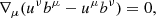
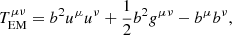
where ∇μ represents the covariant derivative, n is the baryon number density in the fluid frame, uμ is the four-velocity of the gas, u is the internal energy, p is the gas pressure, and bμ is the magnetic four-vector. T is the stress-energy tensor that comprises matter and electromagnetic parts, 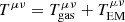 . These can be computed as

where ρ = mn, with m the mean rest mass per particle. The magnetic field B in the observer frame is connected to the magnetic four-vector bμ in such a way that bi = (Bi + btui)/ut, where bt = Biuμgiμ. In the code, we used Gaussian units with the natural unit convention G = c = M = 1, and a factor of  was absorbed into the definition of the Faraday tensor F. Thus, the velocities are dimensionless and the length and time scales can be measured in units of the black hole mass M. Therefore, the length is given in units of rg = GM/c2, and time is given in units of tg = GM/c3. The black hole mass can therefore scale the simulation results.
HARM uses a modified version of the spherical Kerr-Schild (KS) coordinates for its internal grid. In the KS coordinates, the accretion of matter proceeds smoothly through the black hole horizon, and thus, the flow evolution can be tracked properly without encountering coordinate singularities. The grid was adjusted to be logarithmic in radius near the black hole and superexponentially spaced in the outer region to achieve a finer resolution closer to the black hole. In the polar code coordinates, we also added an option to adjust the grid spacing close to the equatorial plane, which can be useful in the evolution of accretion disk flows. In the code, the KS radius r was replaced by the logarithmic radial coordinate x[1], such that
![$$ \begin{aligned} r = e^{x^{[1]}}; \end{aligned} $$](/articles/aa/full_html/2024/07/aa49134-23/aa49134-23-eq8.gif)
the KS latitude θ was substituted by x[2],
![$$ \begin{aligned} \theta = \pi x^{[2]} + \frac{(1-h)}{2}\sin \left(2\pi x^{[2]}\right), \end{aligned} $$](/articles/aa/full_html/2024/07/aa49134-23/aa49134-23-eq9.gif)
and the azimuthal angle ϕ was kept the same, that is,
![$$ \begin{aligned} \phi = x^{[3]}. \end{aligned} $$](/articles/aa/full_html/2024/07/aa49134-23/aa49134-23-eq10.gif)
The outer boundary of the computational domain was set either at 105rg or 104rg in our models so that it did not have any considerable effect on the accretion flows near the horizon, which are the focus of our study. The inner boundary was located at 0.98rH, that is, at a fraction inside the event horizon of the black hole, for the corresponding value of the black hole spin a so that the flow was causally connected. The 2D grid domain had a resolution of 600 × 512 in the (r, θ) directions. For the 3D models, we used a grid resolution of 288 × 256 × 128 in the (r, θ, ϕ) directions. We used a uniform angular resolution for the grid by setting the h parameter to the value 1.0 in Eq. (7) since the flow was initially spherically symmetric.
The adiabatic index was assumed to be that of an ideal gas with γ = 4/3. We used the plasma β parameter, which is defined as the ratio of gas to magnetic pressure (β ≡ pgas/pmag), to initially set either the maximum or minimum magnetic field strength in the domain when the field is enabled, where, pgas = (γ − 1)u and pmag = b2/2. In the models we used, with the initially spherically symmetric Bondi-type inflows, the maximum internal energy of the gas is located near the black hole horizon. We normalized the field strength either by the maximum or minimum value of beta in the domain, as given in Tables 1 and 3. The models with βmax = 0.1 in the domain have a minimum β value of ∼0.0027 at 104rg at the initial time (in comparison with the models with an inclined field with βmin = 0.0003 at 104rg given in Table 3). In the models with the aligned field, the distribution of β along the equator mainly depends on the gas distribution, while in the inclined-field models, they vary in a different fashion in the equatorial region because the geometry of the field is inclined as well. In these models with βmin = 0.0003, the maximum β in the domain is ∼106 near the horizon, and hence, its distribution is smoother than in the aligned-field models.
Summary of models with an aligned field.
2.2. The models and the initial setup
We used the dimensionless spin parameter a to quantify the black hole rotation, with a = 1 being the maximally spinning case. We began our models with a uniform density (of 10−1 in code units) over the entire computational domain with a Kerr black hole at the center and with a zero magnetic field. This configuration was evolved in time; the gas started accreting onto the black hole, and the mass accretion rate increased and reached a quasi-steady value. The evolution of the accretion rate at this stage is plotted in Fig. 1. At this point (at 1000tg given in Fig. 1 for our 2D and 3D models), we introduced the magnetic field of the chosen strength in our code. Similarly, in our 3D models with the inclined field, we introduced a relatively weaker magnetic field at a similar stage to avoid disrupting the gas flow abruptly because the field geometry is inclined to the BH rotation axis.
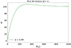 |
Fig. 1. Mass accretion rate at the black hole horizon for the initial part of the simulation before the magnetic field was introduced (β = ∞). The accretion rate initially grows and saturates to a quasi-steady value as time proceeds. It is given in geometric units, which can be scaled to physical units with the black hole mass M. The plot is given for only one spin value, but it is the same for all other values. |
2.2.1. Magnetic field aligned with the rotation axis of the black hole
The uniform magnetic field, which is vertically aligned to the rotation axis of the black hole, is prescribed in the code (the Wald 1974 solution). For this configuration, the magnetic field can be fully described by the only nonvanishing components of the vector potential,
![$$ \begin{aligned} A_t = B_0 a \left[r\Sigma ^{-1}(1+\cos ^2\theta )-1\right], \end{aligned} $$](/articles/aa/full_html/2024/07/aa49134-23/aa49134-23-eq13.gif)
![$$ \begin{aligned} A_{\phi } = B_0\left[\textstyle {\frac{1}{2}}(r^2+a^2)-a^2r\Sigma ^{-1}(1+\cos ^2\theta )\right]\sin ^2\theta , \end{aligned} $$](/articles/aa/full_html/2024/07/aa49134-23/aa49134-23-eq14.gif)
where Σ(r, θ) = r2 + a2cos2θ is a known metric function of the coordinates, and B0 is a constant with the meaning of the magnetic field intensity at a large radius.
We started with 2D models with different spin values, a = 0.99, 0.90, and 0.60, that is, from the near to maximum spin case to a moderate spin, to understand the effect of black hole rotation on the magnetic field and on the outflow development. We used a range of the β-parameter within the flow from 0.1 to 1.0, so that we covered the cases dominated by magnetic pressure and models in which the gas and magnetic pressure initially are at equipartition. We note that the highly magnetized case (β = 0.1) is supposed to exhibit the Meissner-like expulsion of the field lines and its potential influence on the gas flow. Karas et al. (2020) performed a similar study and investigated the very initial stages of the magnetic field and plasma evolution in the presence of a large-scale asymptotically uniform magnetic field. We note here that the original Wald (1974) configuration was determined as an electro-vacuum solution, but we here examine how it is modified at later stages by the presence of matter. With a better-resolved inner region (r ≲ 10 gravitational radii), we indeed confirm that the initial electro-vacuum structure is very quickly canceled because the magnetic field lines are dragged into the black hole event horizon.
The left panels in Fig. 2 show the initial configuration of the model with a black hole spin of a = 0.90 and an initial maximum β = 0.90 in terms of the initial density distribution, the initial geometry of the magnetic field, and also the velocity streamlines.
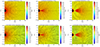 |
Fig. 2. Initial and evolved states of our fiducial model (b01.a90.2D, i.e., with β = 0.1 and a = 0.90) after the magnetic field was turned on, with fluid density in color contours with the magnetic field lines plotted on top (top row) and velocity streamlines overplotted (bottom row). The top panel demonstrates magnetic reconnection events in the equatorial region, and the bottom panel shows the outflows that developed and proceeded outward. |
We also investigated two 3D models for the case of an aligned magnetic field for the models with maximum magnetization (βmax = 0.1) to investigate the nonaxisymmetric effects that can occur in the evolution of the above 2D models and to ensure that they are physically viable. We used the same initial setup as described above. We started from a spherically symmetrically inflow to arrive at a quasi-steady accretion rate. At this point, we introduced the magnetic field given by the Wald (1974) solution and followed the evolution of the system.
2.2.2. Case of an inclined magnetic field
The initial density distributions for these models were obtained in the same way as for the models described in the previous section. Thus, all these models started with a spherically symmetric Bondi-type inflow with a quasi-steady accretion rate. The magnetic field inclined with the rotation axis of the black hole was prescribed according to the form given by Bičák & Janiš (1985). For this configuration, the components of the magnetic field vector in the observer frame are given as
![$$ \begin{aligned}&\mathcal{B} _\phi = A^{-1/2}(\Sigma + 2 Mr)^{-1/2} \Sigma ^{-2} \left\{ 4B_0 M^2 r^2 a^3 (1+\cos ^2 \theta ) \sin \theta \cos \theta \right. \nonumber \\&\qquad - B_1 a [\Sigma ^2(\Sigma + Mr) - 4M^2r^2a^2\sin ^2\theta ]\cos \psi \nonumber \\&\qquad - B_1\left[r\Sigma ^3 - Ma^2 \cos ^2\theta \Sigma ^2 \right. \nonumber \\&\qquad \left. \left. - 2M^2ra^2\sin ^2\theta (r^2 -a^2\cos ^2\theta )\right] \sin \psi \right\} , \end{aligned} $$](/articles/aa/full_html/2024/07/aa49134-23/aa49134-23-eq15.gif)
![$$ \begin{aligned}&\mathcal{B} _\theta = - (\Sigma + 2Mr)^{-1/2} \left\{ B_0 \sin \theta [r + \Sigma ^{-2} a^2M (r^2 - a^2\cos ^2\theta )(1+\cos ^2)] \right. \nonumber \\&\qquad -B_1\cos \theta (r\cos \psi - a\sin \psi ) + B_1 a M \Sigma ^{-2} \cos \theta \nonumber \\&\qquad \times \left[\!\left[ a[r^2 (1+\sin ^2\theta ) + a^4 \cos ^4 \theta ]\cos \psi \right. \right.\nonumber \\&\qquad \left. \left.\left. +r[r^2 + a^2(\cos ^2 \theta - 2 \sin ^2\theta )] \sin \psi \right]\!\right] \right\} , \end{aligned} $$](/articles/aa/full_html/2024/07/aa49134-23/aa49134-23-eq16.gif)
![$$ \begin{aligned}&\mathcal{B} _r = A^{-1/2} \Sigma ^{-2} \left\{ B_0 \cos \theta \left[\!\left[ (r^2 + a^2) [(r^2 - a^2) (r^2 - a^2 \cos ^2 \theta )\right.\right.\right. \nonumber \\&\qquad \left. \left. + 2a^2 r (r-M)(1+\cos ^2\theta )] - a^2\Delta \Sigma \sin ^2\theta \right]\!\right] \nonumber \\&\qquad + B_1 r \Sigma ^2\sin \theta [(r-M)\cos \psi - a\sin \psi ] + B_1 M\sin \theta \nonumber \\&\quad \left. \times [(r^2+a^2)(r^2-a^2\cos ^2\theta ) - \Sigma a^2\sin ^2\theta ] (r\cos \psi - a\sin \psi ) \right\} . \end{aligned} $$](/articles/aa/full_html/2024/07/aa49134-23/aa49134-23-eq17.gif)
The inclination angle with respect to the black hole rotation axis was set by the constants B0 and B1, whose values represent the relative field strengths in the Z (polar) and X directions, respectively. Thus, the inclination angle is given by tan−1(B1/B0). All the models in which the magnetic field was inclined to the black hole rotation axis were run in 3D since they are nonaxisymmetric configurations to begin with.
3. Results
3.1. Models with an aligned magnetic field
A summary of the models we studied is listed in Table 1, and the model names reflect the parameter values we used for them and the setup (2D or 3D). The middle and right columns of Fig. 2 show the evolved states of the fiducial model b01.a90.2D up to a radius of 20rg. In regions below 5rg in these panels, frozen-in magnetic field lines are reconnected while they are accreted onto the black hole.
At the beginning of the simulations (at t = 0tg), the magnetic field lines are expelled from the black hole horizon by the extreme rotation of the black hole. This effect has previously been observed in GRMHD simulations in the case of more extremally spinning black holes (Komissarov & McKinney 2007). As the accretion proceeds according to the initially prescribed Bondi solution, however, the plasma drags the magnetic field along with it to the black hole horizon, and the field lines start to bend in the equatorial region of the flow. As the accretion continues, the idealized initial configuration rapidly evolves into a complex structure with more turbulent field lines in the accreting region near the black hole and more organized field lines in the funnel-like regions close to the rotation axis of the black hole. Thus, the Meissner-like expulsion of the magnetic field lines disappears immediately when the accretion flow begins. Our models also show that this expulsion of the field lines that weakens the Blandford-Znajek mechanism is expected to decrease rapidly in the case of accreting black holes.
The density structures in the bottom middle and right panels of Fig. 2 show the mass outflows that developed in the equatorial region and their velocity directions. This is clearer in the velocity streamlines that are overplotted in the figure. All our magnetized models with an aligned field develop equatorial mass outflows similar to the model depicted in Fig. 2.
The magnetic flux on the black hole horizon was quantified by integrating the radial component of the magnetic field over the horizon and by normalizing it to the inward mass flux,
Figure 3 shows the time-evolution of the magnetic flux on the black hole horizon for models with an initial maximum β = 0.1. The initial flux is high because the initial uniform field strength is much higher than the gas pressure. As the accretion proceeds, this flux diminishes, but maintains values of ϕBH ∼ 30–45 as normalized to the inward mass flux. Values in this range suggest that the accretion is magnetically arrested and further inflow of matter can occur through magnetic reconnection and interchange instabilities.
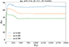 |
Fig. 3. Evolution of the magnetic flux on the black hole horizon with time for the 2D models with initial β = 0.1. |
The mass outflows are sustained in time, as shown in the plot of the outflow rates (again for the models with β = 0.1) in Fig. 4, computed at 10rg. This is the case with all our models with the highly magnetized models showing slightly higher outflow rates when averaged over time than models in which gas and magnetic pressure are in equipartition while being on the same order of magnitude.
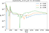 |
Fig. 4. Equatorial mass outflow rate with time at 10rg, after the magnetic field is turned on, for 2D models with β = 0.1 and different spin values. |
Figure 5 shows the inward mass accretion rate at the black hole horizon for the models with β = 0.1. Some quasi-periodic fluctuations in the mass accretion rate and in the magnetic flux on the horizon are visible (in Fig. 3), and these effects seem to depend on the black hole spin. The fluctuating behavior of the flux on the black hole horizon (and in turn, the mass accretion rate) might therefore be caused by the expulsion of the magnetic field lines by a highly spinning black hole. These plots also show that the model with highest black hole spin shows the highest mass outflow rate and the highest mass accretion rate.
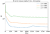 |
Fig. 5. Evolution of the inward mass accretion rate at the black hole horizon with time after the magnetic field is turned on for the model with β = 0.1. |
The models presented in Table 1 show that the black hole spin clearly affects the mass outflow rate. The outflow rates show a systematically increasing pattern, with the black hole spin parameter ranging from a = 0.60 to 0.99 in all models with a varying magnetic field strength. This can partly be attributed to the Meissner-like expulsion of the magnetic field lines by the rotating black holes, which increases with the spin of the black hole. This is in turn reflected in the outflow rates. At the same time, the strength of the magnetization does not show a clear influence on the rate of outflows. All models that vary from β = 0.1 to 1 show similar outflow rates without a clear trend. On the other hand, the black hole spin shows a less pronounced effect on the inward mass accretion rate. The accretion rates reach similar values for the dimensionless spin values of a = 0.60 and 0.90 at all levels of magnetization. It shows slightly higher values for the cases that have near to maximum spin. The Schwarzchild cases show higher accretion rates than the Kerr black holes, however, except in the most highly magnetized case. The table also lists the time-averaged values of the dimensionless flux of the magnetic field on the black hole horizon (ϕBH).
In the last column of Table 1, we list the estimated mass outflow rate for a realistic physical system considering its known parameters. To do this, we converted our results from code units into physical units as follows. Since we used a unit convention of G = c = M = 1 in the code, the length and time units for the simulation results are given by Lunit = GM/c2 and Tunit = GM/c3, respectively. The length and time values can therefore be converted into physical units by using the relevant value of the black hole mass. Table 2 lists the conversion of geometric to physical units considering the black hole mass for M87*. Now, the density unit of the plasma around the black hole is related to the length unit by  so that Mscale depends on the environment under consideration. This density scaling for the AGN accreting environments is rather arbitrary (more so than for GRBs) as the spatial extension of the plasma is large and the density drops by many orders of magnitude from the black hole to the broad-line region (Czerny et al. 2016). In Table 1 we list the outflow rates from our model for the central engine of M87 assuming a black hole mass of 6.2 × 10⁹ M⊙ and a density scaling of ρunit = 8.85 × 10⁻¹⁸ g cm−3 (Janiuk & James 2022).
Example of the conversion of geometric to cgs units. We adopted a black hole mass of M = 6.2 × 10⁹ M⊙ considering M87*.
We note the discontinuities in velocity while the outflow is expanding, which also means that the eruptions are discontinuous. With time, however, the outflows continue toward the outer boundary of the computational domain. The expansion of developed outflows to larger distances in one of our models (b01.a99.2D) is demonstrated in Fig. 6 with velocity streamlines. The flow remains symmetric to the equator over a longer period of time on average, even though some asymmetric behavior with respect to the equator can be observed at certain time instances.
 |
Fig. 6. Density color maps overplotted with the velocity streamlines for one of our representative models, b01.a99.2D, up to a radius of 1000rg showing the outflows extending to larger scales (eventually to the outer boundary of the computational domain) at time t = 500, 750, and 1000tg. The equatorial outflow marked by the outward velocity streamline expands in time as the simulation proceeds. Shocks are visible in the velocity field structure. |
We also investigated two models in 3D with the same initial configuration (for a = 0.90 and 0.99) as for the highly magnetized case (β = 0.1) to account more correctly for the evolution of the system. In Fig. 7, we plot the magnetic flux on the black hole horizon in the case of the 3D models. The values from the 2D models with the same parameters are included for comparison. From this, we note that the flux is slightly lower for the 3D models with the same parameters, but they are both on the same order of magnitude and in the magnetically arrested accretion state as well. Moreover, there are fewer fluctuations in these values for the 3D models. Figure 8 shows the azimuthally averaged equatorial outflow rate with time, computed at 10rg, for the 3D models. They are on the same order of magnitude as in the 2D models, and the time averaged values are given in Table 1. The values listed in the table show that the outflow rate is systematically higher in the two 3D models than in their 2D counterparts. The possibility of outflows along different azimuthal directions might be one reason for this. Thus, our 2D models tend to underestimate the outflow rates. Finally, Fig. 9 shows the inward mass accretion rate at the black hole horizon for the 3D models. The quasi-periodic fluctuations in the accretion rate are more smoothed out in the 3D models, similar to the fluctuations in the magnetic flux.
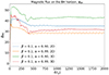 |
Fig. 7. Evolution of the magnetic flux on the black hole horizon with time for the 3D models with β = 0.1 and with different spin values from time t = 1000tg (the values of the 2D models are plotted for comparison). |
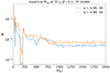 |
Fig. 8. Equatorial mass outflow rate with time at 10rg after the magnetic field is turned on for the 3D models with β = 0.1 and different spin values. |
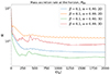 |
Fig. 9. Evolution of inward mass accretion rate at the black hole horizon with time after the magnetic field is turned on for the 3D models with β = 0.1 and different spin values (the values of the 2D models are plotted for comparison). |
Figure 10 shows the initial and the evolved density states in the 3D models. The two top rows show the magnetic field liens for these models plotted on top of the density contours (on the poloidal and equatorial slices), while the two bottom rows show the velocity streamlines at similar time instances of the evolution. As in the 2D models, we also note here that equatorial outflows developed due the magnetic reconnection events in the equatorial region closest to the black hole. By analyzing the equatorial slices, we note that the outflows continue to expand in time.
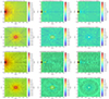 |
Fig. 10. Time evolution of the aligned magnetic field 3D model: selection of exemplary plots showing the density, the magnetic field (top two panels), and velocity (bottom two panels) evolution for the b01.a90.3D model. The equatorial plane (x, y) (view along the rotation axis) and the poloidal section (x, z) (view perpendicular to the rotation axis) are shown. The left panels show the initial configuration with the magnetic field turned on. The middle and right panels show the later evolved states. The first row depicts poloidal slices at ϕ = 0°, and the second row shows equatorial slices (θ = π/2). The third and fourth rows show similar slices for the velocities. |
To better understand the energy composition of the developed outflows, we estimated the radial component ( ) of the matter and electromagnetic parts of the stress-energy tensor, given by Eqs. (4) and (5), for one of our representative models, b01.a90.2D. Figure 11 shows the ratio of the matter and electromagnetic parts of the energy to the total energy. The plots illustrate the case of a matter-dominated equatorial outflow in the initial moments of the simulation (left and middle plots). This can be attributed to plasma that is pushed out along the equatorial direction as the (numerical) reconnection of magnetic field lines begins. At an evolved stage (1000tg, the right plot), the flow is mainly dominated by the electromagnetic contribution due to the persistent current sheet and the continued magnetic reconnection in the equatorial region and the outflows driven by it. The plot on the right also exhibits a higher electromagnetic energy content along the rotation axis of the black hole that is caused by accumulation of magnetic flux near the black hole horizon.
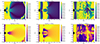 |
Fig. 11. Energy composition of the developed outflows in the representative model b01.a90.2D. The plots show the ratio of the matter (top row) and electromagnetic energy (bottom row) to the total energy at chosen time instances of 20, 30, and 1000tg. While the system is relatively organized at the beginning of the evolution, turbulent behavior gradually prevails in the course of time. Large-scale structures are still seen in the equatorial plane and along the axis, although no well-defined jet develops in this simulation. The value in the color-scale represents a fraction ranging from 0 to 1. |
3.2. Models in which the magnetic field is misaligned with respect to the rotation axis of the black hole
Table 3 summarizes the models we investigated in which the magnetic field was inclined with the rotation axis of the black hole. The model name reflects the magnetic field normalization, the black hole spin, and the inclination angle of the field. As listed in the table, we investigated a set of models with an inclination angle of 45° to the black hole rotation axis. Figure 12 shows the initial and evolved states of the density, the magnetic field, and the velocity field at chosen time instances for the model with a magnetic field inclined at 45°. While the initial magnetic field strength is smaller near the horizon for these models due to the chosen normalization, the Meissner-like expulsion of the field lines is still visible in the top left panel of Fig. 12. As the accretion proceeds and the plasma drags the frozen-in magnetic field lines to the black hole horizon, reconnection events in the equatorial region of the flow in these models become visible, similar to the aligned field lines. As the simulation proceeds, the initially inclined magnetic field tends to align along the black hole rotation axis, as shown in the top middle and right columns of Fig. 12. This in turn affects the development of a more ordered and spread-out outflow, as shown in the plots. The velocity streamlines depicted in the two bottom panels of the figure show that these structured outflows originate in the equatorial region near the black hole horizon and eventually spread out as they move outward. Thus, the outflows developed in these models are not confined to the equatorial region, as is the case of the aligned-field line models.
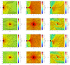 |
Fig. 12. Selection of exemplary moments in the evolution of the 3D model with a magnetic field inclined at 45° to the rotation axis of the black hole, which shows the density, the magnetic field (two top panels), and the velocity (bottom two panels) evolution of the misaligned configuration. The left column shows the initial configuration when we turned the magnetic field on, and the middle and right columns correspond to later time frames, as indicated by the labels attached to each panel. The first row from the top depicts poloidal slices at ϕ = 0°, and the second row shows equatorial slices (θ = π/2). The third and fourth rows show analogous slices with the velocity field. |
Summary of two representative models with the magnetic field inclined with respect to the rotation axis of the black hole.
Figure 13 shows the time evolution of the magnetic flux on the black hole horizon for the inclined-field models. In contrast to the models with an aligned field, here, we started with a field configuration that was weaker near the horizon to avoid disrupting the gas flow. As the accretion proceeded, however, the plasma brought in more magnetic flux to the black horizon and the magnetic flux on the horizon reached values (ϕBH ∼ 30 − 40) very similar to the aligned-field line models. Thus, these models also reach and sustain a magnetically arrested accretion state as accretion proceeds, and the inward accretion rate settles to a value that is similar to the aligned-field line models, as shown in Fig. 14 and Table 3. Thus, the models with misaligned and aligned fields with respect to the black hole spin appear to reach a similar inward accretion rate and a similar magnetic flux on the horizon as the accretion proceeds. While this is true, the velocity patterns developed the in the equatorial region and the plasma distribution seem to be different when the field is misaligned with respect to the spin. This is evident when we compare the velocity stream line plots in the equatorial region in Figs. 10 and 12. This difference is shown more clearly in Fig. 15. The model with the aligned field develops much more turbulent velocity patters in the equatorial region of the flow, while in the inclined-field model, the flow seem to be more streamlined.
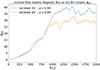 |
Fig. 13. Evolution of the magnetic flux on the black hole horizon with time for the 3D inclined-field models with different spin values. |
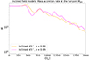 |
Fig. 14. Evolution of the inward mass accretion rate at the black hole horizon with time after the magnetic field is turned on for the 3D inclined-field models. |
 |
Fig. 15. Comparison of velocity patterns at several time instances for the 3D aligned (b01.a90.3D; top row) vs. 3D inclined models (incl45.bmin0003.a90; bottom row) in the inner regions. The plots show that more turbulent structures developed in the equatorial region of the flow in the aligned (top) case, whereas an outflow and a low-density funnel along the spin (vertical) direction emerge in the latter (bottom) case. |
4. Discussion
Several previous works have investigated the inner magnetospheric evolution of black holes and its effect on the observed parameters. They varied in their initial configuration in terms of the matter distribution, the accretion state of the system, and the geometry and strength of the initial magnetic field, however. The configuration investigated by Ressler et al. (2021) is similar to our initial condition because they began from a nonrotating inflow and an asymptotically uniform magnetic field. Their studies were focused on electromagnetic jets that were launched along the rotation axis of the black hole. We introduced the magnetic field in our models in an evolved accretion state that already reached a Bondi-like solution, and we investigated the matter outflows in the equatorial region, mediated by the formation of current sheets, and the velocity patterns there in more detail. This study is significant because the inner magnetopheric evolution, the matter distribution there, and the associated plasmoid-mediated flows there are shown to have effects on the emission that is observed from a region like this (Ripperda et al. 2022). The equatorial outflow rate and the influence of the magnetic field on these flows has not been investigated so far. Several kinetic simulations of the inner black hole magnetosphere, as described in the introduction, support the formation of equatorial current sheets, which in turn supports the outflows and observed flares from supermassive black hole observations (Crinquand et al. 2022; El Mellah et al. 2022, 2023). The results from all our models show persistent magnetic reconnection activity in the inner magnetosphere at ∼5 − 10rg, which in turn supports consistent outflows in the equatorial region. This is evident from the mass outflow rate computed at 10rg for the models with an aligned magnetic field, as shown in Figs. 4 and 8. While being able to capture more physics at smaller scales, PIC simulations have the limitation that the initial magnetic field quickly dies out after a few dozen tg because the current sheet is extended to the outer boundary of the simulation box, which is often provided with open boundary conditions (Crinquand et al. 2021). Because our models are GRMHD simulations, they show persistent reconnection events in the equatorial region and a continued outflow throughout the simulation timescale. Future modeling studies would benefit from a combined approach that involves a coupling of kinetic and fluid approaches, as reported in the experiments initiated by Makwana et al. (2017), for instance.
The 3D GRMHD models discussed in Kwan et al. (2023) required a minimum value of the initial specific angular momentum for the models to reach and sustain a magnetically arrested state. On the other hand, the flows in our models lack any significant angular momentum at the initial or the evolved stages, and they seem to sustain a high amount (> 20 normalized to the inward mass flux, as shown in Figs. 3, and 7) of magnetic flux on the black hole horizon, which is characteristic of a MAD state in the case of disk accretion. Moderate effects of frame dragging are visible in the inner regions of the flow, where the flow and the magnetic field lines are forced to corotate with the black hole. This result is evident in the models with an inclined field as well, where we started with a relatively lower strength of the initial magnetic field.
We note that the initial distribution of β was not uniform in our inclined models due to the Bondi-like distribution of the gas and the resulting gas pressure. It is worth noting that in the models with an inclined field, the regions near the black hole horizon acquired a considerable degree of magnetization with time, as shown in Fig. 13, which depicts the time dependence of the magnetic flux on the horizon. As the models evolved further in time, they also developed outflows, even though they did not specifically focus on the equatorial latitude. This can be attributed to the somewhat differently ordered distribution of the magnetic field lines. Thus, the density patterns developed at later stages in the flow and, consequently, the outflows of matter seem to posses a prevailing inclination similar to the initially imposed field geometry but are also affected by the black hole spin (see Fig. 16). Furthermore, while the general trend on the horizon (in Fig. 13) shows an initial monotonic increase of the magnetic flux due accretion of the frozen-in field lines, the fluctuations caused by the flow instabilities appear to have a magnitude comparable to the effect of spin. The two influences therefore cannot be disentangled.
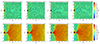 |
Fig. 16. Volume rendered 3D plots show the initial configuration (at zero time in the left panel) and two subsequent more evolved states (at t = 1500tg in the middle panel and t = 2000tg in the right panel). The different color levels indicate the density for the representative run incl45.bmin0003.a90, which covers radii up to 150rg. Starting from the initial Bondi-type inflow at a large distance, an outflow develops and proceeds twisted and inclined with respect to the black hole spin (Z) axis. The color scale ranges from a negligible (close to floor; shown in dark blue) up to a maximum value (red, in code units). |
In the models beginning with an inclined magnetic field, the formation of a low-density vertical funnel region along the rotation axis of the black hole as opposed to no such formation in the aligned magnetic field models was observed. This effect and the associated velocity distribution of matter is depicted in Fig. 15. Our models also suggest variability in density, manifested in terms of variable outflows in a range of ∼10rg. This can be relevant in the context of rapid variability from our own Galactic center Sgr A*, observed within a few to dozens of gravitational radii above the ISCO (GRAVITY Collaboration 2018; Witzel et al. 2021). While we were unable to verify the circular motion of plasmoids (as suggested by the GRAVITY observations), the relevance of strong poloidal magnetic fields in the innermost regions of the flow is evident from our models. The difference in the tilt of the magnetic field also has a significant effect in the turbulence that developed in the flow. This is shown in Fig. 15, where the model with the aligned field depicted in the top row develops much more turbulent velocity patterns in the equatorial region of the flow, while the model with the tilted field develops more streamlined outflows.
5. Summary and conclusions
We investigated the inner magnetospheric structure, the magnetic field evolution, and the flow lines of plasma near the event horizon and the associated outflows that develop in the vicinity of an accreting black hole. The details of some interesting findings can be investigated in more detail in the future. Our results are listed below.
-
The initially uniform magnetic field is promptly dragged by plasma that flows into the black hole even for high magnetization, β ≪ 1, and an almost extreme spin, a → 1.
-
In the aligned 2D and 3D configurations, an equatorial sheet develops, and the magnetic structure suggests an enhanced turbulence and subsequent outflow that diverts a fraction of the accreted material to the outflow.
-
Comparing the 2D simulation results with the corresponding 3D models, we note slightly increased outflow rates that can be attributed to enhanced reconnection events caught by the 3D simulations.
-
The outflow rates have no clear dependence on the magnetic field strength, while the black hole spin seems to have a more considerable effect.
-
In the inclined-field configurations, a low-density funnel develops predominantly along the spin axis rather than in the initial magnetic field direction.
-
At the same time, a dense outflow still persists roughly along the initial inclination of the magnetic field at later stages (in the inclined-field models).
-
The black hole spin has a considerable effect on the flow geometry in all our models, especially in regions near the black hole horizon. This is evident in all models, regardless of the magnetic field inclination. The inclination of the magnetic field only affects the flow geometry at large distances (some hundred rg).
Acknowledgments
We thank Dr. Petra Suková and Dr. Gerardo Urrutia for helpful discussions regarding the presentation of our work. We also greatly acknowledge the anonymous reviewer for very constructive and valuable comments that helped to improve our manuscript. This research was supported in part by the grant DEC-2019/35/B/ST9/04000 from the Polish National Science Center and EXPRO grant 21-06825X from the Czech Science Foundation. The Czech-Polish Mobility program of the two Academies of Sciences, titled “Appearance and dynamics of accretion onto black holes”, is greatly appreciated. We gratefully acknowledge the Polish high-performance computing infrastructure PLGrid (HPC Centers: ACK Cyfronet AGH) for providing computing facilities and support within the computational grant No. PLG/2023/016178. This research was carried out also with the support of the Interdisciplinary Center for Mathematical and Computational Modeling at the University of Warsaw (ICM UW) under the grant Nos. g90-1368 and g92-1500.
References
- Bičák, J., & Janiš, V. 1985, MNRAS, 212, 899 [CrossRef] [Google Scholar]
- Blandford, R. D., & Znajek, R. L. 1977, MNRAS, 179, 433 [NASA ADS] [CrossRef] [Google Scholar]
- Bondi, H. 1952, MNRAS, 112, 195 [Google Scholar]
- Chashkina, A., Bromberg, O., & Levinson, A. 2021, MNRAS, 508, 1241 [NASA ADS] [CrossRef] [Google Scholar]
- Crinquand, B., Cerutti, B., Dubus, G., Parfrey, K., & Philippov, A. 2021, A&A, 650, A163 [NASA ADS] [CrossRef] [EDP Sciences] [Google Scholar]
- Crinquand, B., Cerutti, B., Dubus, G., Parfrey, K., & Philippov, A. 2022, Phys. Rev. Lett., 129, 205101 [NASA ADS] [CrossRef] [Google Scholar]
- Curd, B., & Narayan, R. 2023, MNRAS, 518, 3441 [Google Scholar]
- Czerny, B., Du, P., Wang, J.-M., & Karas, V. 2016, ApJ, 832, 15 [NASA ADS] [CrossRef] [Google Scholar]
- Dermer, C. D., & Menon, G. 2009, High Energy Radiation from Black Holes: Gamma Rays, Cosmic Rays, and Neutrinos (Princeton University Press) [Google Scholar]
- El Mellah, I., Cerutti, B., Crinquand, B., & Parfrey, K. 2022, A&A, 663, A169 [NASA ADS] [CrossRef] [EDP Sciences] [Google Scholar]
- El Mellah, I., Cerutti, B., & Crinquand, B. 2023, A&A, 677, A67 [NASA ADS] [CrossRef] [EDP Sciences] [Google Scholar]
- Event Horizon Telescope Collaboration (Akiyama, K., et al.) 2021, ApJ, 910, L13 [Google Scholar]
- Fender, R., & Gallo, E. 2014, Space Sci. Rev., 183, 323 [NASA ADS] [CrossRef] [Google Scholar]
- Gammie, C. F., McKinney, J. C., & Tóth, G. 2003, ApJ, 589, 444 [Google Scholar]
- GRAVITY Collaboration (Abuter, R., et al.) 2018, A&A, 618, L10 [NASA ADS] [CrossRef] [EDP Sciences] [Google Scholar]
- Hakobyan, H., Ripperda, B., & Philippov, A. A. 2023, ApJ, 943, L29 [Google Scholar]
- Janiuk, A., & James, B. 2022, A&A, 668, A66 [NASA ADS] [CrossRef] [EDP Sciences] [Google Scholar]
- Janiuk, A., Sapountzis, K., Mortier, J., & Janiuk, I. 2018, Supercomput. Front. Innovations, 5, 86 [Google Scholar]
- Karas, V., Sapountzis, K., Janiuk, A., et al. 2020, in Proceedings of RAGtime 20-22: Workshops on Black Holes and Neutron Stars, ed. Z. Stuchlík, et al. (Opava: Silesian University), 107 [Google Scholar]
- King, A. R., Lasota, J. P., & Kundt, W. 1975, Phys. Rev. D, 12, 3037 [CrossRef] [Google Scholar]
- Komissarov, S. S., & McKinney, J. C. 2007, MNRAS, 377, L49 [Google Scholar]
- Kopáček, O., & Karas, V. 2020, ApJ, 900, 119 [Google Scholar]
- Król, D. Ł., & Janiuk, A. 2021, ApJ, 912, 132 [CrossRef] [Google Scholar]
- Kwan, T. M., Dai, L., & Tchekhovskoy, A. 2023, ApJ, 946, L42 [Google Scholar]
- Makwana, K. D., Keppens, R., & Lapenta, G. 2017, Comput. Phys. Commun., 221, 81 [NASA ADS] [CrossRef] [Google Scholar]
- Meier, D. L. 2012, Black Hole Astrophysics: The Engine Paradigm (Heidelberg: Springer, Berlin) [Google Scholar]
- Narayan, R., Igumenshchev, I. V., & Abramowicz, M. A. 2003, PASJ, 55, L69 [NASA ADS] [Google Scholar]
- Narayan, R., & McClintock, J. E. 2015, in General Relativity and Gravitation: A Centennial Perspective, ed. A. Ashtekar, et al. (Cambridge: Cambridge University Press), 133 [Google Scholar]
- Noble, S. C., Gammie, C. F., McKinney, J. C., & Del Zanna, L. 2006, ApJ, 641, 626 [NASA ADS] [CrossRef] [Google Scholar]
- Rees, M. J., & Volonteri, M. 2006, Proc. Int. Astron. Union, 2, 51 [CrossRef] [Google Scholar]
- Ressler, S. M., Quataert, E., White, C. J., & Blaes, O. 2021, MNRAS, 504, 6076 [NASA ADS] [CrossRef] [Google Scholar]
- Ressler, S. M., White, C. J., & Quataert, E. 2023, MNRAS, 521, 4277 [CrossRef] [Google Scholar]
- Ripperda, B., Bacchini, F., & Philippov, A. A. 2020, ApJ, 900, 100 [NASA ADS] [CrossRef] [Google Scholar]
- Ripperda, B., Liska, M., Chatterjee, K., et al. 2022, ApJ, 924, L32 [NASA ADS] [CrossRef] [Google Scholar]
- Suková, P., Zajaček, M., Karas, V., et al. 2023, in Proceedings of RAGtime 23-25: Workshops on Black Holes and Neutron Stars, ed. Z. Stuchlík, et al. (Opava: Silesian University), 109. [Google Scholar]
- Tchekhovskoy, A., Narayan, R., & McKinney, J. C. 2011, MNRAS, 418, L79 [NASA ADS] [CrossRef] [Google Scholar]
- Wald, R. M. 1974, Phys. Rev. D, 10, 1680 [Google Scholar]
- Witzel, G., Martinez, G., Willner, S. P., et al. 2021, ApJ, 917, 73 [NASA ADS] [CrossRef] [Google Scholar]
All Tables
Example of the conversion of geometric to cgs units. We adopted a black hole mass of M = 6.2 × 10⁹ M⊙ considering M87*.
Summary of two representative models with the magnetic field inclined with respect to the rotation axis of the black hole.
All Figures
|
Fig. 1. Mass accretion rate at the black hole horizon for the initial part of the simulation before the magnetic field was introduced (β = ∞). The accretion rate initially grows and saturates to a quasi-steady value as time proceeds. It is given in geometric units, which can be scaled to physical units with the black hole mass M. The plot is given for only one spin value, but it is the same for all other values. |
| In the text | |
|
Fig. 2. Initial and evolved states of our fiducial model (b01.a90.2D, i.e., with β = 0.1 and a = 0.90) after the magnetic field was turned on, with fluid density in color contours with the magnetic field lines plotted on top (top row) and velocity streamlines overplotted (bottom row). The top panel demonstrates magnetic reconnection events in the equatorial region, and the bottom panel shows the outflows that developed and proceeded outward. |
| In the text | |
|
Fig. 3. Evolution of the magnetic flux on the black hole horizon with time for the 2D models with initial β = 0.1. |
| In the text | |
|
Fig. 4. Equatorial mass outflow rate with time at 10rg, after the magnetic field is turned on, for 2D models with β = 0.1 and different spin values. |
| In the text | |
|
Fig. 5. Evolution of the inward mass accretion rate at the black hole horizon with time after the magnetic field is turned on for the model with β = 0.1. |
| In the text | |
|
Fig. 6. Density color maps overplotted with the velocity streamlines for one of our representative models, b01.a99.2D, up to a radius of 1000rg showing the outflows extending to larger scales (eventually to the outer boundary of the computational domain) at time t = 500, 750, and 1000tg. The equatorial outflow marked by the outward velocity streamline expands in time as the simulation proceeds. Shocks are visible in the velocity field structure. |
| In the text | |
|
Fig. 7. Evolution of the magnetic flux on the black hole horizon with time for the 3D models with β = 0.1 and with different spin values from time t = 1000tg (the values of the 2D models are plotted for comparison). |
| In the text | |
|
Fig. 8. Equatorial mass outflow rate with time at 10rg after the magnetic field is turned on for the 3D models with β = 0.1 and different spin values. |
| In the text | |
|
Fig. 9. Evolution of inward mass accretion rate at the black hole horizon with time after the magnetic field is turned on for the 3D models with β = 0.1 and different spin values (the values of the 2D models are plotted for comparison). |
| In the text | |
|
Fig. 10. Time evolution of the aligned magnetic field 3D model: selection of exemplary plots showing the density, the magnetic field (top two panels), and velocity (bottom two panels) evolution for the b01.a90.3D model. The equatorial plane (x, y) (view along the rotation axis) and the poloidal section (x, z) (view perpendicular to the rotation axis) are shown. The left panels show the initial configuration with the magnetic field turned on. The middle and right panels show the later evolved states. The first row depicts poloidal slices at ϕ = 0°, and the second row shows equatorial slices (θ = π/2). The third and fourth rows show similar slices for the velocities. |
| In the text | |
|
Fig. 11. Energy composition of the developed outflows in the representative model b01.a90.2D. The plots show the ratio of the matter (top row) and electromagnetic energy (bottom row) to the total energy at chosen time instances of 20, 30, and 1000tg. While the system is relatively organized at the beginning of the evolution, turbulent behavior gradually prevails in the course of time. Large-scale structures are still seen in the equatorial plane and along the axis, although no well-defined jet develops in this simulation. The value in the color-scale represents a fraction ranging from 0 to 1. |
| In the text | |
|
Fig. 12. Selection of exemplary moments in the evolution of the 3D model with a magnetic field inclined at 45° to the rotation axis of the black hole, which shows the density, the magnetic field (two top panels), and the velocity (bottom two panels) evolution of the misaligned configuration. The left column shows the initial configuration when we turned the magnetic field on, and the middle and right columns correspond to later time frames, as indicated by the labels attached to each panel. The first row from the top depicts poloidal slices at ϕ = 0°, and the second row shows equatorial slices (θ = π/2). The third and fourth rows show analogous slices with the velocity field. |
| In the text | |
|
Fig. 13. Evolution of the magnetic flux on the black hole horizon with time for the 3D inclined-field models with different spin values. |
| In the text | |
|
Fig. 14. Evolution of the inward mass accretion rate at the black hole horizon with time after the magnetic field is turned on for the 3D inclined-field models. |
| In the text | |
|
Fig. 15. Comparison of velocity patterns at several time instances for the 3D aligned (b01.a90.3D; top row) vs. 3D inclined models (incl45.bmin0003.a90; bottom row) in the inner regions. The plots show that more turbulent structures developed in the equatorial region of the flow in the aligned (top) case, whereas an outflow and a low-density funnel along the spin (vertical) direction emerge in the latter (bottom) case. |
| In the text | |
|
Fig. 16. Volume rendered 3D plots show the initial configuration (at zero time in the left panel) and two subsequent more evolved states (at t = 1500tg in the middle panel and t = 2000tg in the right panel). The different color levels indicate the density for the representative run incl45.bmin0003.a90, which covers radii up to 150rg. Starting from the initial Bondi-type inflow at a large distance, an outflow develops and proceeds twisted and inclined with respect to the black hole spin (Z) axis. The color scale ranges from a negligible (close to floor; shown in dark blue) up to a maximum value (red, in code units). |
| In the text | |
Current usage metrics show cumulative count of Article Views (full-text article views including HTML views, PDF and ePub downloads, according to the available data) and Abstracts Views on Vision4Press platform.
Data correspond to usage on the plateform after 2015. The current usage metrics is available 48-96 hours after online publication and is updated daily on week days.
Initial download of the metrics may take a while.