| Issue |
A&A
Volume 687, July 2024
|
|
|---|---|---|
| Article Number | A2 | |
| Number of page(s) | 16 | |
| Section | Astrophysical processes | |
| DOI | https://doi.org/10.1051/0004-6361/202349129 | |
| Published online | 24 June 2024 | |
Impact of disc magnetisation on MHD disc wind signature
1
Astronomical Institute of the Czech Academy of Sciences, Boční-II 1401, Praha 4, Prague 141 00, Czech Republic
e-mail: datta@asu.cas.cz
2
NE 211, IISc, Bengaluru 560012, India
e-mail: write2susmita@gmail.com
3
Univ. Grenoble Alpes, CNRS, IPAG, 38000 Grenoble, France
4
NASA Goddard Space Flight Center, Greenbelt, MD 20771, USA
5
Northwestern University, CIERA, Evanston, IL 60201, USA
6
Friedrich-Alexander-Universität Erlangen-Nürnberg, Erlangen, Germany
7
Dipartimento di Matematica e Fisica, Università degli Studi Roma Tre, Via della Vasca Navale 84, 00146 Roma, Italy
Received:
29
December
2023
Accepted:
19
March
2024
Context. Observations of blue-shifted X-ray absorption lines indicate the presence of wind from the accretion disc in X-ray binaries. Magnetohydrodynamic (MHD) driving is one possible wind-launching mechanism. Recent theoretical developments have made self-similar magnetic accretion-ejection solutions much more generalised, showing that wind can be launched at a much lower magnetisation than the equipartition value, which had previously been the only possibility.
Aims. In this work, we model the transmitted spectra through MHD-driven photoionised wind models with different levels of magnetisation. We investigate the possibility of detecting absorption lines by upcoming instruments, such as XRISM and Athena. We investigate the robustness of the method of fitting asymmetric line profiles by multiple Gaussians.
Methods. We used the photoionisation code XSTAR to simulate the transmitted model spectra. To cover the extensive range of velocity and density of the wind spanned over a large distance (∼105 gravitational radii), we divided the wind into slabs following a logarithmic radial grid. Fake observed spectra are finally produced by convolving model spectra with instrument responses. Since the line asymmetries are apparent in the convolved spectra as well, this can be used in future XRISM and Athena spectra as an observable diagnostic to fit for. We applied some amount of rigor in assessing the equivalent widths of the major absorption lines, including the Fe XXVI Lyα doublets, which will be clearly distinguishable thanks to the superior quality of future high-resolution spectra.
Results. Disc magnetisation stands as another crucial MHD variable that can significantly alter the absorption line profiles. Pure MHD outflow models at low magnetisation are dense enough to be observed by the existing or upcoming instruments. Therefore, these models can serve as simpler alternatives to MHD-thermal models. Fitting with multiple Gaussians is a promising method for handling asymmetric line profiles, as well as the Fe XXVI Lyα doublets.
Key words: accretion, accretion disks / atomic processes / magnetohydrodynamics (MHD) / telescopes / X-rays: binaries
© The Authors 2024
 Open Access article, published by EDP Sciences, under the terms of the Creative Commons Attribution License (https://creativecommons.org/licenses/by/4.0), which permits unrestricted use, distribution, and reproduction in any medium, provided the original work is properly cited.
This article is published in open access under the Subscribe to Open model. Subscribe to A&A to support open access publication.
1. Introduction
Observations of X-ray binaries (XRBs) frequently reveal blue-shifted absorption lines, which are signatures of outflowing wind from the accretion disc (Lee et al. 2002; Miller et al. 2004, 2006a, 2008, 2016; Neilsen & Lee 2009; Ueda et al. 2009; Kallman et al. 2009; King et al. 2012; for review, see Díaz Trigo & Boirin 2016; Ponti et al. 2016). Over the past two decades, XMM-Newton and Chandra (currently NICER and NuSTAR as well) have been providing a wealth of data on winds in X-rays. X-ray winds are mainly observed in highly inclined XRBs during the high-soft state of their outburst (Ponti et al. 2012; Parra et al. 2024). The dependence on the inclination suggests an equatorial geometry. The absence of wind signatures in X-ray spectra, in the canonical hard states, cannot be attributed to mere changes in the illuminating spectra (Lee et al. 2002; Ueda et al. 2009, 2010; Neilsen et al. 2011; Neilsen & Homan 2012) and there is still no consensus about the reason for this dependence on spectral states. Thermodynamic instability could be one possible reason (Chakravorty et al. 2013; Bianchi et al. 2017; Petrucci et al. 2021). Recently wind signatures have been observed in the hard states as well, but in infrared and optical (Rahoui et al. 2014; Muñoz-Darias et al. 2019; Jiménez-Ibarra et al. 2019; Cúneo et al. 2020; Mata Sánchez et al. 2022; Muñoz-Darias & Ponti 2022). This suggests the presence of winds during the entire outburst, albeit with state-dependant changes in the physical properties of the wind. Wind signatures also change from one source to another and, in some cases, for the same source from one observation to another, even in very similar spectral states (e.g. Neilsen & Homan 2012; Parra et al. 2024). This is possibly due to an inhomogeneous medium along the line of sight (LOS).
Matter from the accretion disc around compact objects can be launched via a range of different mechanisms, including magnetohydrodynamic (MHD; Blandford & Payne 1982; Ferreira & Pelletier 1993, 1995; Contopoulos & Lovelace 1994; Contopoulos 1995; Ferreira 1997; Miller et al. 2006b), thermal (Begelman et al. 1983; Woods et al. 1996; Higginbottom et al. 2017; Tomaru et al. 2020; Tetarenko et al. 2020), or radiation (Icke 1980; Shlosman & Vitello 1993; Proga & Kallman 2002; Higginbottom et al. 2024) driving or even a combination (e.g. magneto-thermal Casse & Ferreira 2000, see also Waters & Proga 2018). For XRBs, the matter is highly ionised compared to the winds from AGN which diminishes the line driving possibility and makes the radiation driving inefficient. Both MHD and thermal mechanisms are promising sources for wind driving in XRBs.
At equipartition magnetic field strength, MHD driving is like a bead (matter lifted from the accretion disc) on a wire (the magnetic field line) anchored in the disc and co-rotating with it. If the magnetic field line is sufficiently inclined, the bead is ejected out due to centrifugal force, overcoming the gravitational attraction (Blandford & Payne 1982). The vertical gradient of magnetic pressure can also play a dominant role in launching winds depending on the coupling between different components of the magnetic field. Thermal driving, on the other hand depends on heating the disc material. The scale height of the accretion disc increases with its radius, which makes the outer region inflated and irradiated by the radiation from the central part of the disc. This heats up the material and ejection is achieved when thermal velocity overcomes the escape velocity (Begelman et al. 1983).
Over the last two decades, MHD models developed by two groups, namely (a) Ferreira & Pelletier (1993) and (b) Contopoulos & Lovelace (1994), have been used on several occasions to bridge the gap between theoretical solutions and wind observations in XRBs (Chakravorty et al. 2016, 2023; Fukumura et al. 2010, 2017, 2021, 2022). The primary difference between these two classes of MHD models lies in the connection of the winds with the disc. Accretion-ejection solutions of Ferreira (1997), Casse & Ferreira (2000), Jacquemin-Ide et al. (2019) linked the density of the wind to the disc through the accretion rate, while wind solutions of Blandford & Payne (1982), Contopoulos (1995) treat the density of the wind as a free parameter, independent of the disc. Based on the solutions of Contopoulos & Lovelace (1994), Contopoulos (1995), Fukumura et al. (2017) showed that MHD-driven winds can explain the observation of blue-shifted absorption lines in black hole systems across different mass scales.
The modelling of absorption through a photoionised MHD wind is studied in detail by Chakravorty et al. (2016, hereafter Paper I) where different classes (“cold” and “warm” solutions introduced as CHM and WHM in Sect. 2) of MHD wind solutions are incorporated. The “cold” solutions (Ferreira 1997) are purely MHD winds, whereas “warm” solutions (Casse & Ferreira 2000; Ferreira & Casse 2004) are magneto-thermal since they include external heating at the disc’s surface which aid the MHD forces in lifting outflow material. “Cold” solutions have turned out to be too tenuous and therefore inefficient to reproduce the observed wind signatures, whereas the denser “warm” solutions can indeed reproduce them. A typical 100 ks observation using the upcoming instruments onboard Athena or XRISM can easily detect the wind signatures of “warm” solutions (Chakravorty et al. 2023, hereafter, Paper II) as well as the line asymmetries, which is one of the prominent features of MHD driven winds (Fukumura et al. 2022). However, these “cold” and “warm” solutions were highly magnetised, with a magnetic field energy near equipartition (with thermal pressure). In accretion discs in XRBs, it is expected that the outer region, which contributes mostly in absorption (Chakravorty et al. 2013; Paper I), will have a much lower magnetisation compared to the inner region (Ferreira et al. 2006; Petrucci et al. 2008; Marcel et al. 2018). That is why recently developed generalised “cold” MHD solutions (Jacquemin-Ide et al. 2019) have become crucial in providing denser (compared to high-magnetised “cold” solutions) wind at a lower magnetisation. We may expect that even without the need of any additional disc surface heating, these cold, low magnetised (CLM) solutions possibly will be able to provide the observed equivalent width of absorption lines. In addition, similarly dense solutions are possible at different magnetisations, which further motivates us to study the effect of magnetisation on the transmitted spectra. Thus, this paper is dedicated to exploring the effect of disc magnetisation in the transmitted spectra, while keeping other parameters nearly fixed; this approach is based on the solutions developed by Jacquemin-Ide et al. (2019). We discuss the different classes of accretion-ejection solutions in more detail in Sect. 2.
The plan of the paper is as follows. In Sect. 2, we discuss the theoretical solutions and how different physical constraints are used to select the detectable wind region. The spectrum radiated by the central region of the disc and incident on the wind is constructed in Sect. 3. The mechanism of XSTAR computation is detailed in Sect. 4. Section 5 describes our results, namely, understanding the XSTAR simulated “model spectra” in Sect. 5.1; and analysing the XRISM and Athena-like fake-spectra in Sect. 5.2. A discussion is given in Sect. 6 and our conclusions are presented in Sect. 7. Further details on MHD solutions, incident spectra, and XSTAR computation are given in Appendices A–C respectively.
2. MHD solutions
2.1. Overview of available solutions
An MHD ejection of matter can occur self-consistently along with accretion to the central accretor (Ferreira & Pelletier 1993). In fact, the ejection of matter through the magnetic field line anchored in the disc helps significantly in transporting angular momentum outward and consequently helps in accretion. The basic assumption for these semi-analytical solutions is self-similarity in distance from the black hole (Ferreira & Pelletier 1993).
One major model quantity is the disc ejection efficiency, p, defined as the exponent of the disc accretion rate Ṁa(r) ∝ rp. This exponent1 cannot be larger than unity if ejection is to be powered by accretion alone (Ferreira 1997). It controls the amount of mass lifted from the disc, hence the wind density. The maximum speed achieved along a magnetic surface anchored on a radius, ro, is  , where VKo is the Keplerian speed at ro and λ the magnetic lever arm (Blandford & Payne 1982). It turns out that λ ≃ 1 + 1/2p (Ferreira 1997); thus, depending on the value of the disc ejection efficiency, p, an accretion-ejection solution can be used to model a jet or a wind.
A second very important parameter is the disc magnetisation, μ, defined at the equatorial plane as
where VAz is the vertical component of the Alfvén velocity, Cs is the sound speed, Bz is the vertical component of the large scale magnetic field, μ0 is the magnetic permeability of vacuum, and, Ptot = Pgas + Prad is the sum of the kinetic and radiation pressures. We note that this definition does not include the turbulent magnetic field; namely, it only includes the laminar large scale vertical component present in the disc. As time progresses, different classes of these solutions have been obtained and are outlined one by one of the following.
2.1.1. Cold, highly magnetised (CHM) solutions
It is natural to think that MHD effects will be best able to impact accretion-ejection structures when the magnetic field is near equipartition, with μ between ∼0.1 and 1 (Ferreira & Pelletier 1995). For these cold solutions, namely either isothermal or adiabatic outflows emitted from near-Keplerian thin discs, the typical disc ejection efficiency is found to be around p ∼ 0.01. In Paper I, we studied the physical properties of these CHM solutions (for different possible ejection indices) and concluded that they are not dense enough, regardless of their radial extent, to produce the observed winds.
2.1.2. Warm, highly magnetised (WHM) solutions
One way to have denser winds at same magnetisation is to consider that the surface layers of the disc are heated up by irradiation or MHD turbulence, naturally leading to magneto-thermal models (Casse & Ferreira 2000; Ferreira & Casse 2004). These WHM solutions can produce sufficiently dense observable winds (Paper I). It has also been tested that Athena and XRISM will be able to detect absorption lines from warm MHD outflows and even the line asymmetries should be detected with standard 100 ks observation (Paper II). While the heating of the outer disc surface is actually expected due to irradiation by light coming from the central regions of the disc, these models suffer from the caveat that the amount of extra heating is a free parameter.
2.1.3. CLM (cold, low magnetised) solutions
Garnering progress on the theoretical side of magnetised accretion-ejection solutions, Jacquemin-Ide et al. (2019) showed, for the first time, that significantly denser MHD wind solutions (as dense as WHM solutions) could be achieved with a much weaker magnetic field (μ ranging from ∼10−4 to 0.1), without any requirement for additional heating. At a much smaller magnetic field, ejection resembles a magnetic tower (Ferreira 1997; Lynden-Bell 2003), with a strong toroidal component uplifting the disc material. These CLM solutions are generalised in the sense that they also reproduce the CHM solutions when the strength of the field reaches equipartition (see Figs. 1 and 7 in Jacquemin-Ide et al. 2019).
In the present paper, we focus on these new generalised CLM solutions. Earlier works already showed that although we can ignore the effect of the disc aspect ratio, ϵ (Paper I), the ejection index, p, plays a very dominant role in determining the final transmitted spectra through the wind density (Paper II). With the discovery of the new generalised CLM solutions, a much larger range of magnetisation become accessible to produce the wind. Thus, different dynamics (within the flows) can be achieved with different magnetisation, even if the ejection index remains near constant for those different MHD solutions. In this paper we test the effect of disc magnetisation on MHD disc winds. Hence, we used MHD models whereby the ejection index is fixed to (nearly) the same value p ∼ 0.1, but their magnetisation μ vary through a range of about 1.8 dex.
2.2. Effect of the disc magnetisation on the wind structure
We chose five accretion-ejection CLM solutions with different disc magnetisations: μ = 1.0 × 10⁻³, 2.9 × 10⁻³, 5.9 × 10⁻³, 16 × 10−3, and 67.4 × 10⁻³. All solutions have the same disc aspect ratio, ϵ = H/R = 0.1, the same MHD turbulence parameters, and nearly the same disc ejection efficiency, p ∼ 0.1 (see Appendix A). The outflows are computed assuming isothermal magnetic surfaces, so the winds are “cold” (thermal effects are negligible) and are all of the “magnetic tower” type (see Fig. 7 in Jacquemin-Ide et al. 2019).
Despite the weak magnetic field, the dominant torque leading to accretion remains attributed to the wind (see Fig. 9 in Jacquemin-Ide et al. 2019). This is because MHD turbulence due to the magneto-rotational instability scales with μ1/2 and is also small (see e.g. Salvesen et al. 2016 and references therein). Nevertheless, accretion is subsonic, while the MHD wind carries away a significant portion of the released power (around 50%). Figure 1 shows poloidal cuts of three such solutions: magnetic surfaces in black solid lines and background color showing the ionisation ξ2 (see a discussion in the next section). The spatial oscillations seen in the disc region (within red zone) are characteristic non-linear “channel mode” behaviours due to the magneto-rotational instability (see discussion Sect. 3.1 in Jacquemin-Ide et al. 2019). As μ increases, the disc displays from three (left) to only one (right) oscillations, highly magnetised (near equipartition) solutions having no such oscillations.
 |
Fig. 1. Variation of ξ in the r − z plane for different magnetisations, μ = 0.0059, 0.0160, 0.0674 (from left to right). The Compton-thick region with Nh > 1024.18 along the LOS is shown in red. The white line shows the lowest possible Compton-thin LOS and the value of corresponding i value is given next to it. Black solid lines spread over the whole region are the poloidal magnetic field lines anchored at different radii. Density contours are shown in blue dashed lines. The corresponding log of density (in cc) is written just next to each density iso-contour. |
Since all solutions used here share the same ejection efficiency p ∼ 0.1, the jet asymptotic speed is nearly the same. However, the wind geometry and therefore both velocity and density profiles are actually changing with μ in the acceleration zone near the disc. This is best seen in Fig. 2 where, for each solution, we show only one magnetic surface anchored at 6 Rg (Rg is the gravitational radius). The black solid line is our chosen LOS with an inclination of i = 21°. It can be seen that as μ increases, the magnetic surfaces get more and more vertical (all solutions eventually recollimate toward the axis, Ferreira 1997; Jannaud et al. 2023). This is because the magnetic tension due to the poloidal field increases with μ. Note that this effect has nothing to do with the hoop-stress, which is related to the toroidal field and plays a role only beyond the Alfvén surface. The poloidal magnetic tension, which acts against the inertia of the outflowing plasma and tends to close the magnetic surface, is mostly effective in the sub-Alfvénic region (Ferreira 1997). Thus, along a given LOS, for higher magnetisation solutions, the wind solutions start at slightly closer (see the inset) distances from the black hole.
 |
Fig. 2. Poloidal magnetic field lines for different magnetisations, μ. For each solution we show only one field line anchored at 6 Rg (Rg is the gravitational radius). The solid black line indicates the LOS at an inclination of i = 21° (θ = 69°). Inset shows a zoomed in view of the LOS crossing the magnetic field lines with different magnetisations. We see that the same LOS cuts the different field lines at different distances, due to the different geometry of the magnetic field lines. Please note that the axes of the inset are non-logarithmic. |
The density and the velocity distributions of the wind play crucial roles in deciding the absorption line strength and profile, respectively. The variation of density and velocity along the LOS is shown in Fig. 3. Although the disc magnetisation, μ, affects both the density and velocity, the variations in density (Fig. 3, panel B) are not as significant as those for the velocity profile (Fig. 3, panel A).
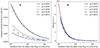 |
Fig. 3. Radial profile of (A) velocity and (B) density of wind along a LOS of i = 21° for different disc magnetisations, μ. Note that although wind is present from a distance of ∼10 Rg from the black hole (inset of Fig. 2), here we only show the part of the wind with a low enough ionisation to contribute significantly to absorption. That is why the radial distance from the black hole extends outwards from ∼500 Rg in this figure. |
It can be seen that, as μ increases, the projected velocity significantly decreases (by factor of 4). This projection effect thus leads to a somewhat counter-intuitive result, namely, that the smaller the magnetic field, the greater the detected wind velocity. This is something to keep in mind when interpreting line profiles.
Note that in Fig. 3, the range of radial distance from the black hole (x-axis) extends outwards from ∼500 Rg. Of course, according to our model formulation, outflowing material exists in the region inwards of ∼500 Rg as well. However, the range emphasised in the figure is for the part of the outflow which has low enough ionisation so that it can “significantly” absorb photons resulting in Fe XXVI (and lower ions) absorption lines in the X-ray spectrum. Discussions in the second paragraph of Sect. 4 and Appendix C.3 detail the method of using a cutoff of log ξ ≤ 6 to select the wind region with low enough ionisation.
2.3. Selection of the LOS for theoretical spectra
In the disc-wind system, optically thin wind is launched from an optically thick disc which lies at the equatorial region. Consequently, for a typical accretion-ejection solution, the LOS that is too close to the equatorial region becomes Compton-thick (NH ≥ 1.5 × 1024 cm−2). This constrains the minimum inclination angle below which wind signatures can not be observed.
On the other hand, if the wind is heavily photoionised, no absorption is possible. Since photoionisation depends inversely on the density, in the polar regions the wind becomes easily over-ionised due to low densities, as can be seen in Fig. 1. Using these two constraints (Compton-thick at low i and over-ionisation at high i), we can find the detectable region of the wind (for more details, see Paper I). In this work, we assume that the disc is extended up to a distance of 105 Rg from the black hole, thereby fixing the distance at which the last magnetic field line is anchored.
We present the spatial distribution of log(ξ) in the r − z plane for μ = 0.0010, 0.0157, and 0.0674 in Fig. 1. The Compton-thick region is shaded in red. The lowest LOS, which is Compton-thin, is shown as a straight white line and the corresponding value of i is mentioned beside it. The density contours are shown in blue dashed lines and the values next to them give an understanding of how density changes with LOS. Paper II showed that variation of LOS can lead to a significant change in the absorption spectra, for MHD models whose density falls fast with increase in i. Here, in this paper, we solely concentrate on the effect of magnetisation on the spectra and hence fixed the LOS at i = 21° throughout the work. The luminosity calculated in Appendix B is used here to find the ionisation distribution.
3. Incident ionising spectrum
The spectral energy distribution (SED), both its shape and normalisation, determines how the material in the outflow will be photoionised, which in turn determines the transmitted spectra. The SEDs of black hole XRBs have two distinct components (Remillard & McClintock 2006; Done et al. 2007): (1) a multi-temperature blackbody component and (2) a non-thermal power-law component. To model the multi-temperature disc component, we have followed the same procedure as mentioned in Bhat et al. (2020). The power-law component had then been added following the prescription of Paper II. The required elaborate details are also recorded in Appendix B. In this section, we offer a summary and present only the necessary parameters for the reader’s information.
To generate the thermal multi-temperature blackbody component of the SED, we use the diskbb model (Mitsuda et al. 1984; Makishima et al. 1986) in XSPEC3 (Arnaud 1996). A hard power-law with a high energy cut-off (hνmax = 100 keV) and low-energy cut-off (hνmin = 20 eV) is then added to diskbb component (fdisk, ν) to generate a fiducial Soft state SED, as follows:
![$$ \begin{aligned} f_{\nu }(\nu )=f_{\rm disk, \nu }(\nu )+\left[A_{\rm pl}\nu ^{-\alpha }\times \exp ^{-\frac{\nu }{\nu _{\rm max}}}\right] \times \exp ^{-\frac{\nu _{\rm min}}{\nu }}. \end{aligned} $$](/articles/aa/full_html/2024/07/aa49129-23/aa49129-23-eq3.gif)
The normalisation factor of the power-law (Apl) is adjusted such that the disc contributes 80% of the 2−20 keV flux. The values of all the parameters involved here and the method in more details are written in Appendix B. The SED prepared above with appropriate normalisation is shown in Fig. 4.
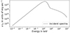 |
Fig. 4. Spectral energy distribution of the ionising radiation emitted from the innermost vicinity of the black hole, and illuminating the wind. |
The self-consistency of the MHD accretion-ejection solutions we are using is that the density of the wind is linked to the disc through the accretion rate. In this work, we impose this consistency between our flow density and the luminosity of the incident SED by assuming that the accretion rate provided in diskbb (to find the luminosity) is the same as that used to find the density (and subsequently, the ionisation) distribution of the wind.
4. Computation using XSTAR
In earlier works (Papers I and II), we used the photoionisation code CLOUDY4 (Ferland et al. 1998, 2017; version C08.00) to compute the transmitted spectra. However, for wind observations from XRB, Fe XXVI Lyα doublet can play a crucial role (Tomaru et al. 2020), which cannot be accurately modelled using CLOUDY (we checked up to the latest version C23.00). Fe XXVI Lyα doublet will be an important part of our analysis in this paper and also all of our subsequent studies on black hole XRB spectra. Hence, we chose XSTAR (version 2.54a) to synthesise the transmitted spectra. For greater flexibility, we used the subroutine version of XSTAR5. Although we followed the usual procedure (Paper I; Fukumura et al. 2017; Paper II), for the sake of completeness, we describe the method in some detail in Appendix C.1 (where we also include a discussion on the input parameters required by XSTAR). To carry out such a study, it is customary to handle the radiation and the wind separately, as explained in Appendix C.3.
To simulate the spectra from the wind which is spread across a large extent (∼105 Rg), we split the wind region into slabs by assuming a logarithmic radial grid ΔRsph/Rsph = 0.115, where ΔRsph is the width of each slab and Rsph is the location (midpoint) of the slab. The choice of the radial resolution is explained in Appendix C.4. For the computation of transmitted spectra from each slab through XSTAR, we need to provide density, column density, and ionisation parameter (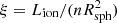 ) of the slab, where Lion is the ionising luminosity illuminating the wind and also the input luminosity parameter in XSTAR. We compute Lion by integrating the incident spectra (Eq. (2)) in the energy range 1−1000 Rydberg and assuming the source to be isotropic (Eq. (B.5)). The calculation of ionising luminosity is further detailed in Appendix B. We already have the rest of the required inputs from Sects. 2 and 3. We thus have a series of slabs whose physical properties are dictated by MHD solution and the ionising radiation. We note that the slabs (and, hence, the outflow) are considered to be present from 6 Rg outwards. However, the ion fraction of Fe XXVI falls below 10% above log ξ = 6 (see Fig. 5 for the solution of μ = 0.0674). Hence, we chose this value of log ξ = 6 as an upper limit for our XSTAR calculations. For each MHD solution and LOS, we found the slab for which log ξ = 6 and we conducted XSTAR calculations from this slab and outwards. Although Lion is the same throughout this work, different density distributions for the different outflow models with different μ make the ionisation distribution different. Consequently, the starting radius for absorption changes. The outflowing MHD wind also has a wide velocity range, as shown in Fig. 3A, which is likely to result in a Doppler shift of the spectrum seen by each slab, as well as the final spectrum seen by the observer. This effect is crucial for creating the shape of the asymmetric line profile due to MHD wind. This whole method of Doppler-shifting the SEDs is similar to what was done in Papers I and II, (Fukumura et al. 2017) and the process is discussed further in Appendix C.2.
 |
Fig. 5. Variation of ion fraction with the ionisation parameter, log ξ for the MHD model of μ = 0.0674 along LOS of i = 21°. Ion fraction drops rapidly at higher ionisation, and at log ξ = 6.0 Fe XXVI becomes less than 10% of Fe, whereas Fe XXV becomes almost zero. Essentially, no absorption will take place for log ξ ≳ 6.0, for these ions. Distance from the black hole is shown in the upper x-axis. We use log ξ = 6.0 as a marker to start the XSTAR computation (Chakravorty et al. 2013). |
5. Results
In this section, we take a deep look at the theoretical spectra computed using Xstar as well as those derived after convolving the theoretical spectra with the instrument responses of XRISM and Athena.
5.1. Model spectra and their variations with μ
5.1.1. Model spectra
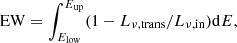
In Fig. 6, we plot the variation in transmitted spectra for the different CLM solutions with varying disc magnetisation. Panel A shows the 6−10 keV spectra, whereas panels B and C focus on the Fe XXV and Fe XXVI line, respectively. These XSTAR output spectra are termed as model spectra to distinguish from fake-spectra generated using instruments’ response later.
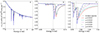 |
Fig. 6. Variation of transmitted spectra for different magnetisations. The angle of the LOS is i = 21° from the plane of the disc. The cutoff of log ξ = 6 sets the inner boundary. The outer boundary is set by the field line anchored on the disc at a distance of 105 Rg from the black hole. Broadband view of 6−10 keV is presented in panel A indicating the most prominent absorption lines are Fe XXV and Fe XXVI, zoomed in view of which are shown in panels B and C respectively. Rest frame energy of Fe XXV resonance line (6.70040 keV) in panel B and, Fe XXVI Lyα1 (6.97316 keV) and Lyα2 (6.95197 keV) in panel C are indicated by the vertical grey lines. Magnetisation clearly plays a decisive role in shaping the transmitted spectra. |
Fe XXVI is one of the very few ions that shows significant absorption features in this heavily ionised medium, and due to spin-orbit coupling, Fe XXVI Lyα line splits into doublet with rest frame energy at 6.952 and 6.973 keV. Figure 6C focuses on the Fe XXVI Lyα doublet. Panel B concentrates on the Fe XXV absorption line. In both panels we notice that the blue shift and the broadening of the line increases significantly with decreasing magnetisation. This result was hinted by the evolution of wind velocity with disc magnetisation, seen in Fig. 3A in Sect. 2.2. In this section, we analyse how the physical parameters of the outflow can influence the extent of absorption and results in the line profiles that we are seeing.
5.1.2. Absorption measure distribution
The most suitable way to understand the variations in the line profiles (as a function of μ) is to study the absorption measure distribution (AMD; Holczer et al. 2007; Behar 2009) which is the variation of absorption with respect to the ionisation parameter, ξ. The popular way to represent the AMD is to plot the “equivalent” hydrogen column density along the LOS as a function of log ξ. To focus on a specific ion, the hydrogen column density can be replaced by the ionic column density. For Fe XXVI ion, we can write:

Here, dNFe XXVI represents the Fe XXVI ionic column density of each slab in our computation, and d(log ξ) is the ionisation spread within the slab. The advantage of using AMD(ξ) is that for self-similar wind solutions, AMD(ξ) [or any other AMD(x)] becomes independent of the slab’s width and scales only with ξ [the physical parameter x]. For details, we refer to Sect. 3 of Behar (2009).
Panel A of Fig. 7 shows the AMD(ξ)’s. We see that irrespective of the MHD model, maximum absorption occurs from slabs with log ξ ∼ 5.3, indicating the well established fact that absorption is driven by ionisation distribution. The upper limit of log ξ = 6.0 where all the AMDs have their cut-off, arises due to the choice we made (see last paragraph in Sect. 4 for details). At the lower limit, different AMDs are cut off at different values of ξ – even if we consider the disc to be 105 Rg for all models. This is because of the varying geometry of the flow (varying shapes of the field lines) we get different densities for different μ solutions (Fig. 3B).
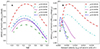 |
Fig. 7. For Fe XXVI, AMD(ξ) versus log ξ is plotted in panels A and B shows the AMD(vout) with respect to vout. |
However, the ionisation parameter does not relate the absorption to the more direct physical parameters, namely, the velocity and density of the outflow. We chose to extend the concept of AMD as a function of outward velocity (vout), or LOS velocity of the wind, as shown in panel B of Fig. 7. We chose the physical parameter velocity since velocity is reflected directly in high-resolution spectra as blue-shifts of absorption lines or as the spread and asymmetry in the line profiles. We immediately see that unlike the different AMD(ξ)’s that had more or less similar shape, the different AMD(vout)s end up being diverse in terms of shape. The peak of the ones with lower μ is at higher velocities and the AMDs are also spread over a much larger velocity range. For example, the peak of the AMD(vout) moves from 0.001c for the model with μ = 0.0674 to 0.006c for the one with μ = 0.0010. For these respective models, the velocity range Δvout over which absorption is happening also increases from 0.005c to 0.02c. The effect is directly reflected in the corresponding line spectra. This is most prominently seen in Fig. 6C, particularly via the Fe XXVI Lyα1 line, which is the most (least) blue shifted for the μ = 0.0010 (0.0674) model and has the largest (smallest) spread and asymmetry in the line profile. For an asymmetric line profile it is challenging to calculate its blue-shift. Since the peak of the AMD(vout) denotes maximum absorption, one can crudely state that the velocity of that physical region of the outflow will most significantly influence the blue shift of the absorption line. In Sect. 6.3, we make an attempt to compare the maximum theoretical velocity of the wind with the maximum velocity that can be traced by fitting the asymmetric lines in the fake-spectra with multiple Gaussian components.
In Fig. 6C we can easily notice the two distinct lines of Fe XXVI Lyα doublet, more so for the higher magnetisation solutions with μ = 0.0059, 0.0160, 0.0674. Since absorption occurs through a much larger velocity range for lower magnetisation solutions, the individual lines in the doublet suffer through more smearing out due to gradual Doppler broadening. Hence for lower magnetisation solutions, the distinction between the doublet features are less apparent, but still present.
Figure 6A tells us that for 6−10 keV energy range, rest of the absorption lines are quite weak relative to the Fe XXV and Fe XXVI ones. We have further checked (not shown in the figure) that all absorption lines below 6 keV (for the physical scenario considered in this paper) are also weak. Quantifying how much weaker these lines are goes beyond the scope of this paper and we shall attempt such an analysis in future publication, including the fitting of actual observations. Therefore, in the rest of the paper, whenever we present quantitative measures of absorption, we are focussing only on the Fe XXV lines and the Fe XXVI Lyα doublet. Below, we present calculations of the equivalent widths of the lines in the model spectra.
5.1.3. EW from model spectra
To calculate the equivalent width (EW) of any absorption line within the model spectra, we need to find the difference in the area under the incident (Lν, in) and transmitted (Lν, trans) spectra corresponding to that line. We define the EW as follows:
Elow and Eup are the lower and upper bound of the energy range over which the absorption line is spread. For Fe XXV, Elow = 6.69 keV, Eup = 6.82 keV and for Fe XXVI, Elow = 6.94 keV, and Eup = 7.15 keV. Following this procedure, we estimate the EW for Fe XXV and the composite Fe XXVI (consisting of the doublet) absorption lines, which are represented in Table 1, for the various magnetisations considered in this paper.
However, to distinguish between the two components within the Fe XXVI Lyα doublet (Lyα1 at 6.973 keV, Lyα2 at 6.952 keV), we need to make our procedure more sophisticated. Because of Doppler broadening the right wing of Lyα2 (due to higher velocity absorbing gas) overlaps with the Fe XXVI Lyα1 (due to lower velocity absorbing gas), thus blending the two lines into the resultant profile. This is true for all the MHD models that we consider in this paper. In Fig. 8, we demonstrate our attempt to separate out the two lines using the following method. We extend the right wing of Fe XXVI Lyα2 using a slope which is the average of the gradients (of the SED) of last two energy grid points available just before the profile falls into the trough of Fe XXVI Lyα1. This gives us the best estimate of the line profile for Fe XXVI Lyα2, and following the procedure mentioned above, we measure the EW of it. By subtracting the EW of Fe XXVI Lyα2 from the total EW of Fe XXVI Lyα doublet, we eventually find the EW of Fe XXVI Lyα1. The estimated EW of Lyα1, Lyα2 and their ratio from model spectra are shown in Table 2.
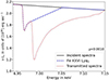 |
Fig. 8. Within the line profile of the Fe XXVI Lyα doublet structure (dotted, red), from the model spectrum (for the MHD model with μ = 0.0010), we find the best approximation for the Fe XXVI Lyα2 line (in dashed blue). |
Ideally, the ratio of EW for Lyα1/Lyα2 should be 2.0 if the absorption line is in the linear regime of curve of growth. If the absorption reaches to saturation regime, the ratio becomes lesser than 2.0. This fact is reflected from the lower values of Lyα1/Lyα2 for model spectra for μ = 0.0160 and 0.0674 solutions due to very narrow velocity range over which absorption occurs and reaches the saturation regime. Lyα1/Lyα2 values greater than 2.0 indicates that we have underestimated the EW of Lyα2.
5.2. XRISM and Athena-like view of the spectra
In this section, we check whether the instruments with superior spectral resolution onboard XRISM and Athena are sufficient to detect the absorption lines, including the resolved doublet line profiles. We further attempted multiple Gaussian fitting within the fake-spectra to handle highly asymmetric and complicated line profiles.
5.2.1. Fake-spectra as proxies for future observations
We convolved the model spectra with XRISM (Tashiro 2022) and Athena (Barret et al. 2023) response for a typical standard exposure time of 100 ks using the FAKEIT command in XSPEC. Assuming the same distance to the source (8 kpc) chosen in Sect. 3, the observed flux is 3.15 × 10⁻⁹ ergs cm−2 s−1 (∼132 mCrab) for all the μ values. After convolving the spectra with the instrument’s response6, we always rebinned the spectra using the FTGROUPPHA tool in XSPEC setting grouptype = opt, which implements an optimal binning scheme following Kaastra & Bleeker (2016). The convolved spectra for μ = 0.0010 along with the continuum model (diskbb+power-law) is shown in Fig. 9, and indicates clearly that XRISM with 100 ks exposure will be able to detect the Fe XXV and Fe XXVI absorption lines. The proposed Athena telescope has an effective area ∼0.20 m2 (Bavdaz et al. 2018) at 6 keV compared to that of XRISM which is ∼0.03 m2 at 6 keV (XRISM Science Team 2020). This fact is reflected in the counts of the convolved spectra for XRISM and Athena (Fig. 10). Thus, all physical parameters remaining same, the same absorption line will be detected by Athena with much lower exposure time; or for the same exposure time, Athena can provide better statistics on line asymmetries.
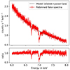 |
Fig. 9. Spectrum along i = 21° through the MHD model with μ = 0.0010 convolved with XRISM response function for 100 ks exposure. The source has a flux of 3.15 × 10⁻⁹ ergs cm−2 s−1 (∼132 mCrab) (consistent with the incident spectra generated in Sect. 3), and corresponds to a total number of 800 photon counts in the energy range 6.0−8.0 keV. Top: simulated spectra (solid, red line) along with the model (diskbb+power-law; dashed, black line) to fit the continuum after the optimal binning. Bottom: ratio of data and model. |
5.2.2. EW from fake-spectra
To estimate EW from the observed spectra, it is typical to fit the absorption line with a Gaussian. However, for magnetically driven wind, the asymmetric absorption line shape cannot be fitted well by a single Gaussian; thus, multiple Gaussian components become necessary to fit one absorption line (method used in Paper II). The Gaussian components are added till the ftest7 probability of adding another Gaussian component becomes below 90%. Figure 10 shows the use of this method, for μ = 0.0010, to fit the Fe XXV (left panels) and Fe XXVI (right panels) absorption lines. We then add the EWs of the constituent Gaussians to get the effective EW of the absorption line. Results are presented in Table 1 along with 90% confidence range (within brackets). Estimated EWs from model spectra for all the cases lie within the range of 90% confidence limit. This implies that even if the lines are asymmetric and have very complicated profiles, the multiple Gaussian fitting methods can correctly measure of the actual strength of absorption and be proxy of the physics involved. If rigorous quantification of the individual lines of the Fe XXVI Lyα doublet complex is required, then we would need even better fitting methods. While it is beyond the main scope of the paper, we briefly describe a demonstration in Sect. 6.2.
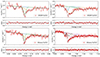 |
Fig. 10. Fitting the Fe XXV (left) and Fe XXVI (right) absorption line in the fake-spectra (red, plus symbols) of XRISM (top) and Athena (bottom) with multiple Gaussians components. The fake-spectra correspond to 100 ks observations along i = 21° through the MHD model with μ = 0.0010. Each fit also shows the constituent Gaussian components. The total model is shown in black dashed line. The higher photon counts indicates Athena’s higher effective area. The shape of the line profile is captured more accurately by Athena because of higher energy resolution. The ratio of data/model is shown at the bottom of each fit. |
6. Discussion
6.1. MHD versus MHD-thermal outflow models
In Papers I and II, we found that only WHM solutions (which included “external” heating at the disc surface) were likely to yield blue-shifted absorption lines, compatible with those observed in high resolution spectra of XRBs. Further, as stated earlier as well, all those solutions (even the cold ones considered in those papers) had a high disc magnetisation, μ. We can think of the WHM solutions as MHD-thermal outflow models that were found to be “effective”, whilst the cold solutions (which were pure MHD solutions) were not dense enough. However, we see in this paper that, since the variety of pure MHD cold solutions have been enhanced by introduction of the CLM solutions, these new solutions are dense enough to produce detectable absorption lines. In this section, we attempt to make a comparison between these two kinds of solutions (WHM and CLM solutions) to better understand the relevant (for observables like absorption lines in XRBs) parameter space of MHD solutions.
We chose the WHM solution with the closest values for p(= 0.1) and ϵ(= 0.07) compared to that of the CLM solutions [p ∼ 0.1 and ϵ = 0.1] that have been used in the previous sections of this paper8. According to Paper I, the slight difference in the disc thickness (ϵ) should not introduce any significant change in the wind signatures. The WHM solution has a disc magnetisation of μ = 0.074, which is at the lower end of near-equipartition solutions. Nevertheless, by comparing it with our CLM solution with μ = 10−3, it provides a stark contrast in disc magnetisation (as intended). Both the outflow models were subject to the same illuminating SED (hence, with the same disc accretion rate). However we allowed the inclination angle to vary. While the CLMs use a LOS i = 21°, we chose a LOS i = 12° for the WHM because our analysis showed that although these solutions are different, it was these LOSs that provided similar LOS density profile. This is because the larger the μ the larger is the accretion speed. Hence, for the same disc accretion rate, the CLM displays a denser disc, hence, a denser wind.
The observable of concern for us is the absorption line(s). As we show in the comparison in Fig. 11, it will be impossible to distinguish between these two models in a real observation. While the existence of an external heating due to irradiation seems reasonable, and thereby, the existence of magneto-thermal winds from the outer regions of accretion discs, the same wind signatures can be accounted for by pure MHD (CLM) winds. Here, obviously, a degeneracy between the plausible models crops up, particularly if the inclination is unknown or poorly constrained. Addressing such degeneracy is beyond the scope of this paper and we shall attempt such exercises in later publications where we shall fit actual observations.
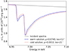 |
Fig. 11. Comparison between transmitted spectra for the WHM (μ = 0.0740) solution and the CLM (μ = 0.0010) solution. Note: to keep the density profile similar, a different LOS (closer to the disc) has been chosen for the WHM solution. Both solutions are illuminated with the same SED and the disc has the same accretion rate. |
6.2. Ratio of Fe XXVI Lyα from fake-spectra
The right panels of Fig. 10 seem to indicate that Fe XXVI doublet line profile needs finer fitting methods than that used in Sect. 5.2.2. It is difficult to separate out some of the component Gaussians and assign to either Lyα1 or Lyα2 – these “problematic” components have significant overlap in the energy ranges of both the lines of the doublet. Here we show another finer attempt with the aim to get some measure of the separate EW of the two lines of the doublet.
We restricted the hard limit for the width of the constituent Gaussians to 5 eV. Furthermore, we applied this method to the higher resolution Athena fake-spectra only, where the two lines of the doublet complex are easier to distinguish than in the XRISM fake-spectra. The fit for μ = 0.0010 (same fake-spectra as in bottom right panel of Fig. 10) is presented in Fig. 12. Fe XXVI Lyα2 (a lower energy component of the doublet) is always fitted by one or two narrow Gaussians, and no Gaussian overlaps between Lyα1 and Lyα2. Hence, a simple addition of EWs of the constituent Gaussians can now give us estimates of separate EWs of Lyα1 and Lyα2. For all the μ values, the EWs and their 90% confidence range, estimated through this procedure are given in Table 2.
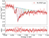 |
Fig. 12. Fitting the Fe XXVI Lyα absorption line in the fake-spectra for Athena with multiple Gaussians while the hard limit of the line width of each Gaussian component is fixed to 5 eV. The fake-spectra are computed for μ = 0.0010, assuming 100 ks observation of Athena (same as bottom right panel of Fig. 10). The total model is shown in black dashed line while the different Gaussian components are in different colors (solid lines). |
We note that in this method, we lose information on any plausible large velocity tail of the Lyα2 that may exist within the energy range of the Lyα1 line. Thus, this method suffer from the risk of underestimating the EW of Lyα2 and overestimating the EW of Lyα1. The line ratios are given in the last two columns of Table 2. We note that the line ratios in this method are far higher than what was calculated using the previous “theoretical” method using the model spectra (Sect. 5.1.3). The difference between the line ratios predicted from model spectra and Athena fake-spectra decreases gradually with increasing magnetisation. This is not a surprising trend because, with increasing magnetisation, the lines become narrower (less velocity spread, Fig. 6C); hence, the contamination from Lyα2 inside the energy range of Lyα1 is lower. This is a general problem to estimate the EW of any absorption line whenever it is polluted by some other line. The methods that we have described may be made more accurate using the velocity information available in the outflow models. However such endeavours will come at the cost of loss of generality and is also beyond the scope of this paper.
6.3. Maximum velocity of wind from fake-spectra
Typically, MHD winds are expected to create broad asymmetric Fe XXVI absorption lines because the wind is present and hence absorb over a wider (than thermal winds) range of velocity. From the fits (in Sect. 6.2), if we compare the line centre of the most energetic Gaussian component with the rest frame energy of the Fe XXVI Lyα1 line (6.97316 keV), we can get an estimate of the maximum velocity at which the wind is moving. Since, in this paper, we know a priori at what maximum velocity the wind starts to absorb (slab closest to black hole along LOS), this value can be compared to the one derived from the fake-spectra. Such a comparison can help us assess how well the Athena observations can reflect the real physical scenario. The result of this exercise is presented in Table 3. We find that fitting with Gaussian components whose widths are constrained to less than 5 eV gives us very good agreement to the “real” wind – indicating that such (or similar) techniques are quite promising to model asymmetric line profiles.
Comparison of maximum velocity of absorbing gas along LOS estimated (a) directly from MHD models (Col. 2), and (b) by fitting Fe XXVI Lyα1 line in Athena fake-spectra with multiple Gaussians whose widths are restricted to 5 eV (Col. 3).
7. Concluding remarks
In this work, we have simulated, using XSTAR, the transmitted spectra of CLM (cold low magnetised) solutions of a new kind. These purely MHD winds are cold (isothermal) outflows emitted from the outer disc regions where a CLM solution is assumed to be settled. We varied the disc magnetisation, μ, and looked for its influence on wind signatures, if any. Besides the disc magnetisation, μ, the five accretion-ejection solutions used in this work share the same disc aspect ratio, disc ejection efficiency, p ≃ 0.1, and MHD turbulence properties. The key findings are summarised below.
(1) The CLM solutions can produce significant absorption lines. This is due to the fact that for the same disc accretion rate, weakly magnetised discs launch winds that are denser than those from highly magnetised (near-equipartition) discs. With lowering the magnetisation, field lines become more bent and the LOS projected velocity increases, leading to a broader and more blue-shifted absorption line. Differences in disc magnetisation can therefore lead to very different line profiles.
(2) Upcoming instruments such as XRISM and Athena, with a typical 100 ks exposure time, will be able to detect not only the absorption line, but also the line asymmetries (assuming the MHD wind is produced from the entire disc surface), which are crucial features of MHD winds.
(3) For an asymmetric absorption line, fitting with multiple Gaussians is a good technique – not only for estimations of equivalent widths, but also to asses physical quantities such as the velocity.
(4) The asymmetry of the absorption line strongly depends on the velocity range over which absorption occurs, namely, the radial extension of the wind. The MHD wind can be produced only from the outer part of the disc which seems now plausible due to weakly magnetised wind. In that case, even with MHD wind, we may not see asymmetric line profile. However, this is not explicitly demosntrated in this paper.
(5) The CLM accretion-ejection solutions (pure MHD) can give rise to spectra similar to those obtained for WHM solutions (thermal MHD). This can be obtained by allowing for a slight variation of the LOS (much less than typical observational uncertainty) and likely by also playing with other model parameters (which have been kept constant in our study). Thus, WHM winds are no longer necessary to describe the observed wind signatures in XRBs.
 , where Lion is the ionising luminosity illuminating the wind, n is the density of the wind, and Rsph is the distance of the wind from the ionising source, discussed in detail in Sect. 4.
See Appendix D for the details of the response files used here and the comparison with the ones recently released during the review process of this paper. The main difference is a significant decrease in the effective area for both instruments, meaning that the exposure time used here should be significantly increased (100% for XRISM and 40−50% for Athena) to reach the same signal-to-noise ratio (S/N).
The WHM solutions used in Paper II had ϵ = 0.01 and MHD parameters αm = 2, 𝒫m = 1, while values used here are αm = 𝒫m = 1 (see Appendix A for more details).
Acknowledgments
S.R.D. thanks for the support from the Czech Science Foundation project GACR 21-06825X and the institutional support from RVO:6798581. P.O.P., M.P., J.F., N.Z. and M.C. acknowledge financial support from the High Energy National Programme (PNHE) of the national french research agency (CNRS) and from the french spatial agency (CNES). S.B. and M.P. acknowledge support from the European Union Horizon 2020 Research and Innovation Framework Programme under grant agreement AHEAD2020 No. 871158, from PRIN MUR 2022 SEAWIND 2022Y2T94C, supported by European Union – Next Generation EU, and support from INAF LG 2023 BLOSSOM.
References
- Arnaud, K. A. 1996, in Astronomical Data Analysis Software and Systems V, eds. G. H. Jacoby, & J. Barnes, ASP Conf. Ser., 101, 17 [NASA ADS] [Google Scholar]
- Barret, D., Albouys, V., Herder, J.-W. D., et al. 2023, Exp. Astron., 55, 373 [NASA ADS] [CrossRef] [Google Scholar]
- Bavdaz, M., Wille, E., Ayre, M., et al. 2018, in Space Telescopes and Instrumentation 2018: Ultraviolet to Gamma Ray, eds. J. W. A. den Herder, S. Nikzad, & K. Nakazawa, SPIE Conf. Ser., 10699, 106990X [NASA ADS] [Google Scholar]
- Begelman, M. C., McKee, C. F., & Shields, G. A. 1983, ApJ, 271, 70 [CrossRef] [Google Scholar]
- Behar, E. 2009, ApJ, 703, 1346 [NASA ADS] [CrossRef] [Google Scholar]
- Bhat, H. K., Chakravorty, S., Sengupta, D., et al. 2020, MNRAS, 497, 2992 [NASA ADS] [CrossRef] [Google Scholar]
- Bianchi, S., Ponti, G., Muñoz-Darias, T., & Petrucci, P.-O. 2017, MNRAS, 472, 2454 [Google Scholar]
- Blandford, R. D., & Payne, D. G. 1982, MNRAS, 199, 883 [CrossRef] [Google Scholar]
- Blum, J. L., Miller, J. M., Cackett, E., et al. 2010, ApJ, 713, 1244 [NASA ADS] [CrossRef] [Google Scholar]
- Casse, F., & Ferreira, J. 2000, A&A, 361, 1178 [NASA ADS] [Google Scholar]
- Chakravorty, S., Lee, J. C., & Neilsen, J. 2013, MNRAS, 436, 560 [Google Scholar]
- Chakravorty, S., Petrucci, P. O., Ferreira, J., et al. 2016, A&A, 589, A119 [NASA ADS] [CrossRef] [EDP Sciences] [Google Scholar]
- Chakravorty, S., Petrucci, P.-O., Datta, S. R., et al. 2023, MNRAS, 518, 1335 [Google Scholar]
- Contopoulos, J. 1995, ApJ, 450, 616 [NASA ADS] [CrossRef] [Google Scholar]
- Contopoulos, J., & Lovelace, R. V. E. 1994, ApJ, 429, 139 [NASA ADS] [CrossRef] [Google Scholar]
- Cúneo, V. A., Muñoz-Darias, T., Sánchez-Sierras, J., et al. 2020, MNRAS, 498, 25 [CrossRef] [Google Scholar]
- Díaz Trigo, M., & Boirin, L. 2016, Astron. Nachr., 337, 368 [Google Scholar]
- Done, C., Gierliński, M., & Kubota, A. 2007, A&ARv, 15, 1 [Google Scholar]
- Ferland, G. J., Korista, K. T., Verner, D. A., et al. 1998, PASP, 110, 761 [Google Scholar]
- Ferland, G. J., Chatzikos, M., Guzmán, F., et al. 2017, Rev. Mex. Astron. Astrofis., 53, 385 [NASA ADS] [Google Scholar]
- Ferreira, J. 1997, A&A, 319, 340 [Google Scholar]
- Ferreira, J., & Casse, F. 2004, ApJ, 601, L139 [NASA ADS] [CrossRef] [Google Scholar]
- Ferreira, J., & Pelletier, G. 1993, A&A, 276, 625 [NASA ADS] [Google Scholar]
- Ferreira, J., & Pelletier, G. 1995, A&A, 295, 807 [NASA ADS] [Google Scholar]
- Ferreira, J., Petrucci, P.-O., Henri, G., Saugé, L., & Pelletier, G. 2006, A&A, 447, 813 [NASA ADS] [CrossRef] [EDP Sciences] [Google Scholar]
- Fukumura, K., Kazanas, D., Contopoulos, I., & Behar, E. 2010, ApJ, 715, 636 [NASA ADS] [CrossRef] [Google Scholar]
- Fukumura, K., Kazanas, D., Shrader, C., et al. 2017, Nat. Astron., 1, 0062 [NASA ADS] [CrossRef] [Google Scholar]
- Fukumura, K., Kazanas, D., Shrader, C., et al. 2021, ApJ, 912, 86 [NASA ADS] [CrossRef] [Google Scholar]
- Fukumura, K., Dadina, M., Matzeu, G., et al. 2022, ApJ, 940, 6 [NASA ADS] [CrossRef] [Google Scholar]
- Higginbottom, N., Proga, D., Knigge, C., & Long, K. S. 2017, ApJ, 836, 42 [Google Scholar]
- Higginbottom, N., Scepi, N., Knigge, C., et al. 2024, MNRAS, 527, 9236 [Google Scholar]
- Holczer, T., Behar, E., & Kaspi, S. 2007, ApJ, 663, 799 [NASA ADS] [CrossRef] [Google Scholar]
- Icke, V. 1980, AJ, 85, 329 [NASA ADS] [CrossRef] [Google Scholar]
- Jacquemin-Ide, J., Ferreira, J., & Lesur, G. 2019, MNRAS, 490, 3112 [Google Scholar]
- Jannaud, T., Zanni, C., & Ferreira, J. 2023, A&A, 669, A159 [NASA ADS] [CrossRef] [EDP Sciences] [Google Scholar]
- Jiménez-Ibarra, F., Muñoz-Darias, T., Casares, J., Armas Padilla, M., & Corral-Santana, J. M. 2019, MNRAS, 489, 3420 [Google Scholar]
- Kaastra, J. S., & Bleeker, J. A. M. 2016, A&A, 587, A151 [NASA ADS] [CrossRef] [EDP Sciences] [Google Scholar]
- Kallman, T. R., Bautista, M. A., Goriely, S., et al. 2009, ApJ, 701, 865 [NASA ADS] [CrossRef] [Google Scholar]
- King, A. L., Miller, J. M., Raymond, J., et al. 2012, ApJ, 746, L20 [NASA ADS] [CrossRef] [Google Scholar]
- King, A. L., Miller, J. M., Raymond, J., et al. 2013, ApJ, 762, 103 [Google Scholar]
- Lee, J. C., Reynolds, C. S., Remillard, R., et al. 2002, ApJ, 567, 1102 [NASA ADS] [CrossRef] [Google Scholar]
- Lesur, G., Ferreira, J., & Ogilvie, G. I. 2013, A&A, 550, A61 [NASA ADS] [CrossRef] [EDP Sciences] [Google Scholar]
- Luminari, A., Tombesi, F., Piconcelli, E., et al. 2020, A&A, 633, A55 [NASA ADS] [CrossRef] [EDP Sciences] [Google Scholar]
- Lynden-Bell, D. 2003, MNRAS, 341, 1360 [NASA ADS] [CrossRef] [Google Scholar]
- Makishima, K., Maejima, Y., Mitsuda, K., et al. 1986, ApJ, 308, 635 [NASA ADS] [CrossRef] [Google Scholar]
- Marcel, G., Ferreira, J., Petrucci, P.-O., et al. 2018, A&A, 617, A46 [NASA ADS] [CrossRef] [EDP Sciences] [Google Scholar]
- Marcel, G., Ferreira, J., Clavel, M., et al. 2019, A&A, 626, A115 [NASA ADS] [CrossRef] [EDP Sciences] [Google Scholar]
- Mata Sánchez, D., Muñoz-Darias, T., Cúneo, V. A., et al. 2022, ApJ, 926, L10 [CrossRef] [Google Scholar]
- Miller, J. M., Raymond, J., Fabian, A. C., et al. 2004, ApJ, 601, 450 [NASA ADS] [CrossRef] [Google Scholar]
- Miller, J. M., Raymond, J., Homan, J., et al. 2006a, ApJ, 646, 394 [NASA ADS] [CrossRef] [Google Scholar]
- Miller, J. M., Raymond, J., Fabian, A., et al. 2006b, Nature, 441, 953 [NASA ADS] [CrossRef] [Google Scholar]
- Miller, J. M., Raymond, J., Reynolds, C. S., et al. 2008, ApJ, 680, 1359 [NASA ADS] [CrossRef] [Google Scholar]
- Miller, J. M., Fabian, A. C., Kaastra, J., et al. 2015, ApJ, 814, 87 [NASA ADS] [CrossRef] [Google Scholar]
- Miller, J. M., Raymond, J., Fabian, A. C., et al. 2016, ApJ, 821, L9 [CrossRef] [Google Scholar]
- Mitsuda, K., Inoue, H., Koyama, K., et al. 1984, PASJ, 36, 741 [NASA ADS] [Google Scholar]
- Muñoz-Darias, T., & Ponti, G. 2022, A&A, 664, A104 [NASA ADS] [CrossRef] [EDP Sciences] [Google Scholar]
- Muñoz-Darias, T., Jiménez-Ibarra, F., Panizo-Espinar, G., et al. 2019, ApJ, 879, L4 [CrossRef] [Google Scholar]
- Neilsen, J., & Homan, J. 2012, ApJ, 750, 27 [NASA ADS] [CrossRef] [Google Scholar]
- Neilsen, J., & Lee, J. C. 2009, Nature, 458, 481 [NASA ADS] [CrossRef] [Google Scholar]
- Neilsen, J., Remillard, R. A., & Lee, J. C. 2011, ApJ, 737, 69 [Google Scholar]
- Parra, M., Petrucci, P. O., Bianchi, S., et al. 2024, A&A, 681, A49 [NASA ADS] [CrossRef] [EDP Sciences] [Google Scholar]
- Petrucci, P.-O., Ferreira, J., Henri, G., & Pelletier, G. 2008, MNRAS, 385, L88 [NASA ADS] [CrossRef] [Google Scholar]
- Petrucci, P. O., Bianchi, S., Ponti, G., et al. 2021, A&A, 649, A128 [NASA ADS] [CrossRef] [EDP Sciences] [Google Scholar]
- Ponti, G., Fender, R. P., Begelman, M. C., et al. 2012, MNRAS, 422, L11 [NASA ADS] [CrossRef] [Google Scholar]
- Ponti, G., Bianchi, S., Muñoz-Darias, T., et al. 2016, Astron. Nachr., 337, 512 [Google Scholar]
- Pringle, J. E. 1981, ARA&A, 19, 137 [NASA ADS] [CrossRef] [Google Scholar]
- Proga, D., & Kallman, T. R. 2002, ApJ, 565, 455 [NASA ADS] [CrossRef] [Google Scholar]
- Rahoui, F., Coriat, M., & Lee, J. C. 2014, MNRAS, 442, 1610 [Google Scholar]
- Remillard, R. A., & McClintock, J. E. 2006, ARA&A, 44, 49 [Google Scholar]
- Salvesen, G., Simon, J. B., Armitage, P. J., & Begelman, M. C. 2016, MNRAS, 457, 857 [Google Scholar]
- Shakura, N. I., & Sunyaev, R. A. 1973, A&A, 24, 337 [NASA ADS] [Google Scholar]
- Shlosman, I., & Vitello, P. 1993, ApJ, 409, 372 [NASA ADS] [CrossRef] [Google Scholar]
- Tashiro, M. S. 2022, Int. J. Mod. Phys., D, 31, 2230001 [NASA ADS] [CrossRef] [Google Scholar]
- Tetarenko, B. E., Dubus, G., Marcel, G., Done, C., & Clavel, M. 2020, MNRAS, 495, 3666 [Google Scholar]
- Tomaru, R., Done, C., Ohsuga, K., Odaka, H., & Takahashi, T. 2020, MNRAS, 494, 3413 [NASA ADS] [CrossRef] [Google Scholar]
- Trueba, N., Miller, J. M., Kaastra, J., et al. 2019, ApJ, 886, 104 [NASA ADS] [CrossRef] [Google Scholar]
- Ueda, Y., Yamaoka, K., & Remillard, R. 2009, ApJ, 695, 888 [NASA ADS] [CrossRef] [Google Scholar]
- Ueda, Y., Honda, K., Takahashi, H., et al. 2010, ApJ, 713, 257 [NASA ADS] [CrossRef] [Google Scholar]
- Waters, T., & Proga, D. 2018, MNRAS, 481, 2628 [NASA ADS] [Google Scholar]
- Woods, D. T., Klein, R. I., Castor, J. I., McKee, C. F., & Bell, J. B. 1996, ApJ, 461, 767 [NASA ADS] [CrossRef] [Google Scholar]
- XRISM Science Team 2020, arXiv e-prints [arXiv:2003.04962] [Google Scholar]
- Zimmerman, E. R., Narayan, R., McClintock, J. E., & Miller, J. M. 2005, ApJ, 618, 832 [NASA ADS] [CrossRef] [Google Scholar]
Appendix A: MHD solutions
The dynamics of accretion-ejection structures is intricate and complex due to the coupling between the disc and wind/jet, as well as the very involvement of the magnetic field (Ferreira & Pelletier 1995; Ferreira 1997; Jacquemin-Ide et al. 2019). Here, we briefly attempt to explain the difference between highly (CHM) and weakly (CLM) magnetised cold solutions, but the interested reader is referred to these papers.
The disc is assumed to be the locus of an MHD turbulence that leads to the presence of anomalous viscosity and magnetic diffusivities. The origin of such a turbulence is probably the magneto-rotational instability (hereafter, MRI), which provides a viscosity that scales with μ1/2 (see e.g. Salvesen et al. 2016 and references therein). Such a scaling appears to be consistent with the values chosen for the MHD turbulence parameters that were used in our self-similar solutions, namely αm = 1 or 2 and a turbulent magnetic Prandtl number of unity. While viscosity provides a torque, thereby allowing accretion to proceed (although the wind torque is usually dominant), magnetic diffusivity allows the plasma to cross the field lines, so that a steady-state situation can be achieved.
CHM accretion-ejection solutions, with μ ranging from 0.1 to unity, are such that MRI is marginally quenched as the MRI wavelength is of the order of the disc’s scale height. Angular momentum transfer from the disc to the outflowing wind by the large scale magnetic field can then also be seen as some sort of MRI process. Instead of leading to turbulence in that case, the non-linear stage of the instability is the jet launching (Lesur et al. 2013). When the magnetic field is much weaker (μ between 10−4 and 0.1), MRI leads to the formation of non-linear channel modes within the disc, that are manifested as steady-state spatial oscillations of all disc quantities (that can be seen in Fig. 1) and leads to the generalised CLM solutions. The number of oscillations depends on the MRI wavelength (Jacquemin-Ide et al. 2019). However, despite the presence of the turbulent torque, the wind still carries away a significant portion, b = 2Pjet/Pacc, of the accretion power, Pacc, released in the disc. For all solutions used in this paper, Table A.1 provides a number of physical quantities associated with them. We note that the first five solutions are isothermal (i.e. CLM) and emitted from a disc with an aspect ratio of ϵ = 0.1 and turbulence of αm = 1. The sixth solution is a WHM solution emitted from a disc with ϵ = 0.07 and αm = 2, where the total thermal energy represents only 7.5% of the MHD power carried away. Although it would be preferable to choose solutions with the same input parameters, namely, identical values of ejection index (p), similar MHD turbulence parameters and disc aspect ratio (ϵ), no WHM solution with p = 0.1 and ϵ > 0.07 is available.
Parameters and quantities associated with the six solutions used in this paper: disc magnetisation, μ, ejection index, p, midplane sonic Mach number, ms, fraction, b of the accretion power carried away by the two outflows, ratio, fjet, of heat deposition per unit mass in the jet to Bernoulli integral, normalised jet mass load, κ, magnetic lever arm, λ (Blandford & Payne 1982) and colatitude, θA, of the Alfvén point in degrees.
Some of the involved MHD parameters are more dominant than the others in determining (and hence, causing variations in) the strengths and shapes of the absorption lines. In Papers I and II, we found the model spectra are largely dominated by the ejection indices p (density stratification) of the MHD outflow. The LOS angle variation and the change in size of the disc also showed some effect on the final model spectra (Paper II), but their influence was found to be less than that of p. In this paper we are keen in finding the influence of the variation of magnetisation, μ; hence, we have chosen solutions having similar p values. We found that a variation in μ has indeed a significant effect in changing the absorption lines because of its influence on the wind geometry and projected velocity.
Moreover, it should be noted that different p values are possible within a very narrow interval for μ (see Fig. 7 in Jacquemin-Ide et al. 2019). Thus, throughout the investigations of Paper II and this one, we realise that there may be possibilities of degeneracy between input MHD parameters in the future, when we try to fit observed data with our models. However, it is beyond the scope of this paper to assess how strong those degeneracies will be and/or whether it is possible to break some of the degeneracies using constraints from other analysis methods (e.g. knowing the LOS to the source from optical light dipping analysis). In addition to the parameters of the MHD model, uncertainty in the input parameters of XSTAR can also induce changes in the model spectra which is elaborately written in Appendix C.5.
Appendix B: Details of the SED modelling and ionising luminosity
The spectral energy distribution (SED) of black hole XRB has two distinct components (Remillard & McClintock 2006; Done et al. 2007): (1) multi-temperature blackbody component and (2) non-thermal power-law component. During different states of the outbursts, the BHXBs show varying degrees of contribution from the components mentioned above. According to the definition of Remillard & McClintock (2006), the state where the multi-temperature blackbody component dominates and contributes more than 75% of the 2-20 keV flux is termed as Soft state, whereas in the hard state, this contribution drops below 20%.
To prepare the radiation component from the accretion disc, we follow the same procedure as mentioned in Bhat et al. (2020). A standard model to estimate the flux due to the thermal multi-temperature blackbody component of the SED is diskbb (Mitsuda et al. 1984; Makishima et al. 1986) in XSPEC9 (Arnaud 1996). The required input parameters for diskbb to generate the observed flux are:
the temperature at the innermost radius of the disc (Shakura & Sunyaev 1973; Pringle 1981) and
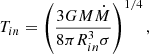
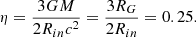
the normalisation due to distance and inclination. Here, we assume the mass of the black hole as M = 10 M⊙, the accretion rate as M = 0.1 ṀEdd, the innermost radius of the disc as Rin = 6RG (RG is the gravitational radius), the distance to the source as D = 8 kpc, and the angle between the LOS and the normal to the plane of the disc as θ = 70° (i = 20°). Here, G is the gravitational constant, σ is the Stefan-Boltzmann constant. To define ṀEdd, we need to define accretion efficiency (η) in the equation:

For the model of diskbb, zero torque is assumed at the inner boundary of the disc, which is termed as the standard torque scenario in Zimmerman et al. (2005). Following Eq. (10) of Zimmerman et al. (2005) for standard torque scenario and comparing with our Eq. (B.3), we get
This is the same method as mentioned in Bhat et al. (2020) to find the flux using diskbb. We use this value of η to find Ṁ in physical unit from ṀEdd as
where LEdd is the Eddington luminosity. Following the whole procedure, we find Tin = 0.56 keV as well as the flux per unit frequency fdisk, ν(ν) from the accretion disc as a function of frequency (ν).
Following Paper II, a hard power law with a high-energy cut-off (hνmax = 100 keV) is added to fdisk, ν(ν) to mimic the typical observed SED (Eq. (2)). We focus only on the soft state of the accretion flow and prepare the incident SED accordingly, as outflowing winds are observed primarily in the softer state of the accretion flow (Miller et al. 2008; Neilsen & Lee 2009; Blum et al. 2010; Ponti et al. 2012). Following Remillard & McClintock (2006), the energy index α is set to 1.5 (i.e. photon index, Γ, up to 2.5), normalisation factor, Apl, is adjusted to 3.11× 10⁻⁹ at or above 2 keV, and to (3.11/1.0005)× 10−9 below 2 keV, such that the disc contributes 80% of the 2-20 keV flux and the rest comes from the power law. An exponential lower energy cut-off (hνmin = 20 eV) is introduced to diminish the contribution of the power law in the lower energy regime. For more details, see Paper II.
The luminosity radiated from the central regions of the accretion disc is what ionises the wind material. To derive this ionising luminosity, we simply integrate the model SED within the 1-1000 Ryd energy range and then multiply it by 4πD2 (D = 8 kpc being the distance between the source and observer):
where fν(ν) is given by Eq. (2). We find that Lion = 9.87 × 1037 ergs sec−1. The incident SED normalised appropriately with Lion is shown in Fig. 4. The ionisation parameter, ξ, is calculated using Lion for each slab depending on its density and distance, and is used as input in our XSTAR calculations. We note that in general, Eq. (B.5) should also have had a correction factor pertaining to the LOS angle of the observer. However, here the model SED was prepared for an inclination angle of i = 20° and we are studying the transmitted spectra at 21°, thus rendering this correction factor redundant.
Appendix C: Details of XSTAR computation
C.1. Inputs to XSTAR
For the requirement of the photoionised cloud to be in thermal equilibrium, XSTAR10 computes the temperature and all other physical quantities of interest, for instance, the ion fractions, by taking into account all possible heating and cooling mechanisms. A single computation of XSTAR assumes the photoionised cloud to have constant density. However along the LOS through the wind, the density and velocity decreases with increasing distance from the black hole following the profiles prescribed by the given MHD solution. The anchoring radius of magnetic field lines for launching wind spans a wide distance range, from 6 RG to ∼105-106RG. Therefore, we have to split the whole wind region into slabs by assuming a logarithmic radial grid ΔRsph/Rsph = 0.115, so that each slab has ‘near constant’ density. The justification of the chosen radial resolution is discussed in Appendix C.4. Here, ΔRsph is the width of each slab and Rsph is the location (mid point) of the slab in radial coordinate assuming the disc in the equatorial plane at θ = 90° (i = 0°) and the black hole is at the center of the spherical polar coordinate. The density (n) of each slab is fixed to the density of the wind at that location (Fig. 3(B)). The column density (Nh) of each slab is calculated depending on the density and ΔRsph.
The atomic physics calculations within XSTAR depend on the flux FXSTAR(ν), whose SED is obviously the same as that of the input SED, but the normalisation is decided by Lion (Eq. B.5) provided as an input to XSTAR. To calculate flux from luminosity, XSTAR always assumes a spherical geometry of the cloud around the source leading to the dilution of flux from luminosity by  , where Rsph is the distance of the slab from the central source.
The abundance of the wind (and hence each slab) is set to solar abundance. We always fix the turbulent velocity parameter in XSTAR to be zero throughout the whole study in this work. Resolution of energy grid is set to quite high value of 63599 for all the calculations to keep the theoretical resolution finer than the energy resolution of upcoming instruments onboard, XRISM and Athena. Other required parameters for XSTAR, namely, the minimum electron abundance, threshold ion abundance, and so on, are kept at default values.
With the specified radial and energy resolution, computation of final transmitted spectra for one MHD solution takes run time ∼3-4 hours. The run time of XSTAR is almost proportional to the resolution of energy grid.
C.2. Doppler shifting the spectrum
The outward velocities of the slabs are set according to the velocity profile of the wind (Fig. 3(A)). This bulk velocity of wind Doppler shifts the spectra along LOS. The first slab is moving away from the central region of the disc. Therefore, the SED prepared in Section (3) is red-shifted using the velocity of the first slab (i.e. the one with log ξ = 6). For rest of the slabs, transmitted spectra from one slab is fed as the incident spectra of the next slab after Doppler-shifting appropriately depending on the velocity difference between the two slabs. We note that the output spectrum from each slab carries the signatures of the absorption caused by the various ions in the slab. The spectra from the last slab is blue-shifted according to its outward velocity to get the final observed spectrum. For more details about the procedure, we refer to Paper I and Paper II, Fukumura et al. (2017). The wind velocities we are considering are also too small to produce any relativistic Doppler correction in flux (Luminari et al. 2020).
C.3. Decoupled radiation zone and wind zone of accretion disc
To produce the final transmitted spectrum, we assume that the radiation generated from the accretion disc passes through the wind, which is also launched from the disc. This physical picture remains consistent with our method of calculation only because we can ignore (i) the outer region of the disc as a source of radiation and (ii) the inner region of the wind as a significant contributor to absorption. The radiation emitted by the accretion disc (following the Shakura-Sunyaev temperature profile) within a distance of ∼100Rg from the black hole is almost equal to the total radiation emitted by the disc. The compact size of the hot corona emitting hard X-ray power-law is also in line with this (Marcel et al. 2019).
On the other hand, the wind near the black hole is heavily ionised due to its close proximity to the source of most energetic X-rays, thus rendering the contribution from this part of the wind as insignificant in the absorption spectrum. To proffer a quantitative idea of the absorption, we show the Fe XXVI and Fe XXV ion fraction as a function of ionisation in Fig. 5 for the MHD model with μ = 0.0674 along a LOS of i = 21°. Ion fraction of Fe XXV becomes almost zero, and Fe XXVI falls much below 0.1 in the inner region (∼500Rg) of the wind indicating a negligible contribution in absorption (also see Chakravorty et al. 2013). Although, MHD outflow is present from the black hole horizon (according to our model calculations), still, upto distances ∼500-1000 Rg from the black hole, the gas will not contribute to absorption. Absence of Fe XXV and Fe XXVI due to over-ionisation confirms the absence of other ‘lower’ ions (whose ionisation potentials are at lower energy compared to that for Fe XXV and Fe XXVI) as well. Note that we have kept the ‘higher ions’ (e.g. He-like and H-like Neon ions) out of discussion here, because they are beyond the scope of this paper.
C.4. Slab size
The MHD wind covers a large range of velocity and density, which requires us to split the LOS into multiple individual zones that can be approximated by slabs. A higher number of slabs leads to more precise computation but will also be significantly more computationally expensive. We thus use the energy resolution of the telescope set as reference we should follow to optimally simulate the spectra. The wind velocity plays a major role in making the absorption line asymmetric, which is one of the key properties of MHD-driven wind. That is why in Paper I and II, wind along the LOS is divided depending on the criterion of velocity difference (or resolution) between two consecutive slabs which was set to 75 km/s at ∼6.5 keV (to keep it finer than the expected resolution of XRISM (300 km/s) and Athena (150 km/s) at 6.5 keV).
The inner region of the wind has large outflow velocity compared to outer region (Fig. 3(A)). Using the criterion of velocity resolution splits the inner region of the wind in larger number of slabs compared to that at the outer region. However we know that the outer region contributes more to absorption due to lower ionisation of the wind material there. Therefore, from the point of view of contribution in absorption, outer region should be populated with more slabs (in the physical model) to provide more correct prescription of the density of wind which is used by XSTAR in estimating the final spectra. The large range in the radial distance (∼105Rg) also necessitates the use of a logarithmic grid. All these considerations prompted us to choose a constant value of ΔRsph/Rsph as a criterion to split the wind into slabs. Following Fukumura et al. (2017), we assumed ΔRsph/Rsph = 0.115. However, it is equally important to check if the velocity difference between two consecutive slabs remains lesser than or equal to the resolutions of XRISM and Athena (≲150 km/s). For the MHD models that we use, except for the very inner region (first 4-5 slabs out of ∼45), which also contributes the least in absorption, the velocity difference between two consecutive slabs always remains below 150 km/s.
C.5. Uncertainties in input parameters
Possible uncertainties in the MHD model are mentioned in Appendix A. Moreover, there are also variants within XSTAR calculation, which can induce some changes in the model spectra. In the following, we record those effects, although a deeper quantitative analysis on those is beyond the scope of this paper.
Geometry: geometry of the wind is quite uncertain which dictates how much the wind covers the incident radiation, covering fraction (in XSTAR, this is denoted as cfrac). Covering fraction governs the escape probability of continuum radiation in inward and outward direction. If the radiation source is completely covered by the photoionised slab (i.e. cfrac = 1), then continuum emission in the inward direction eventually reenters the slab and the whole continuum transmits in the outward direction. Similar to continuum, this fact decreases the strength of absorption lines as well because emission lines from the other parts of the cloud adds up over the transmitted absorption lines. The reduction of strength of absorption due to covering fraction is nicely shown in Figure 4 of Trueba et al. (2019). The dependency on covering fraction is discussed in detail in Appendix F (“Recombination Continuum Emission and Escape”) of XSTAR manual11. It is also very natural that radiation from LOS will be lost due to Thomson scattering as it traverses through the wind, which has been included recently in XSTAR (version 2.54a and above). The loss of radiation from LOS is a function of covering fraction and similarly as earlier, there will be no loss due to scattering for a completely closed geometry. Therefore, for partially covered geometry, due to escaping of continuum in inward direction as well as due to loss of scattering, continuum along LOS will be reduced. Reduction in the continuum flux will decrease the ionisation of the wind and which typically will increase the absorption in our cases. Summing up, uncertainty in the geometry of the wind puts uncertainty in the absorption line profile. In past works (King et al. 2013; Miller et al. 2015; Trueba et al. 2019), an average value of 0.5 is assumed. In this work, we assume completely closed geometry (cfrac = 1) to estimate the line profile and this gives the lower limit of absorption as decreasing the covering fraction will increase the absorption.
Turbulent velocity of the gas: for the MHD wind, absorption happens over a large velocity range (Δv ∼ 0.02c) and, hence, the absorption lines have significant Doppler broadening even when the gas medium is considered to be entirely photoionised. However, if there is enough thermal energy in the medium to compete with the extent of the Doppler broadening, then a considerable value of turbulent velocity can also change the absorption line profile (Fukumura et al. 2010).
Appendix D: Response files of XRISM and Athena for fake-spectra simulations
The redistribution matrix file and ancillary response file (i.e. rmf and arf) used to simulate the XRISM spectra shown in this paper are ‘xarm_res_h7ev_20170818.rmf’ and ‘xarm_res_pnt_pa_20170818.arf’ and correspond to the old hitomi matrices. They were the official ones before February 2024. However, the current official files are named ‘rsl_Hp_5eV.rmf’ and ‘rsl_pointsource_GVclosed.arf’. They are available at https://heasarc.gsfc.nasa.gov/docs/xrism/proposals/responses.html12. The energy resolution is similar to the one we used, but the effective area is now very different due to the gate valve issue as shown at the top of Fig. D.1.
 |
Fig. D.1. Top: Comparison of effective area for XRISM between two sets of arf, one which is used in this paper to simulate fake-spectra (black dashed line) and one which is available as the latest on February, 2024 (red dotted line). Bottom: Same as above but for Athena. |
For the Athena simulations, we use ‘XIFU_CC_BASELINECONF_2018_10_10.rmf’ as redistribution matrix file and ‘XIFU_CC_BASELINECONF_2018_10_10.arf’ as ancillary response file in this work. They are available on the website directory of http://x-ifu-resources.irap.omp.eu/PUBLIC/OLDRESPONSESBEfOREREFORMULATION/CCCONFIGURATION/13 of X-IFU resources. These files have been revised recently and the official ones available in Feb. 2024 i.e. ‘athena_xifu_3eV_gaussian.rmf’ and ‘athena_xifu_13_rows_no_filter.arf’ are in the website directory http://x-ifu-resources.irap.omp.eu/PUBLIC/NEWATHENARESPONSEANDBACKGROUNDFILES/14. The energy resolution of this latest rmf file is 3 eV at 7 keV compared to 2.5 eV for the response used in this work. There is also a significant change in the effective area as shown at the bottom of Fig. D.1.
The paper review is occurring very close to the release of the new rmf and arf files of XRISM and Athena. Therefore, we were not able to use them in the present version of the paper. Since the changes are mainly decrease of effective area, to obtain simulated spectra with similar S/N as shown in this paper, one would just have to compensate by increasing the exposure time, when using the new response files. One has to increase the exposure time by 100% for the XRISM simulations and by 40-50% for Athena simulations.
All Tables
Comparison of maximum velocity of absorbing gas along LOS estimated (a) directly from MHD models (Col. 2), and (b) by fitting Fe XXVI Lyα1 line in Athena fake-spectra with multiple Gaussians whose widths are restricted to 5 eV (Col. 3).
Parameters and quantities associated with the six solutions used in this paper: disc magnetisation, μ, ejection index, p, midplane sonic Mach number, ms, fraction, b of the accretion power carried away by the two outflows, ratio, fjet, of heat deposition per unit mass in the jet to Bernoulli integral, normalised jet mass load, κ, magnetic lever arm, λ (Blandford & Payne 1982) and colatitude, θA, of the Alfvén point in degrees.
All Figures
|
Fig. 1. Variation of ξ in the r − z plane for different magnetisations, μ = 0.0059, 0.0160, 0.0674 (from left to right). The Compton-thick region with Nh > 1024.18 along the LOS is shown in red. The white line shows the lowest possible Compton-thin LOS and the value of corresponding i value is given next to it. Black solid lines spread over the whole region are the poloidal magnetic field lines anchored at different radii. Density contours are shown in blue dashed lines. The corresponding log of density (in cc) is written just next to each density iso-contour. |
| In the text | |
|
Fig. 2. Poloidal magnetic field lines for different magnetisations, μ. For each solution we show only one field line anchored at 6 Rg (Rg is the gravitational radius). The solid black line indicates the LOS at an inclination of i = 21° (θ = 69°). Inset shows a zoomed in view of the LOS crossing the magnetic field lines with different magnetisations. We see that the same LOS cuts the different field lines at different distances, due to the different geometry of the magnetic field lines. Please note that the axes of the inset are non-logarithmic. |
| In the text | |
|
Fig. 3. Radial profile of (A) velocity and (B) density of wind along a LOS of i = 21° for different disc magnetisations, μ. Note that although wind is present from a distance of ∼10 Rg from the black hole (inset of Fig. 2), here we only show the part of the wind with a low enough ionisation to contribute significantly to absorption. That is why the radial distance from the black hole extends outwards from ∼500 Rg in this figure. |
| In the text | |
|
Fig. 4. Spectral energy distribution of the ionising radiation emitted from the innermost vicinity of the black hole, and illuminating the wind. |
| In the text | |
|
Fig. 5. Variation of ion fraction with the ionisation parameter, log ξ for the MHD model of μ = 0.0674 along LOS of i = 21°. Ion fraction drops rapidly at higher ionisation, and at log ξ = 6.0 Fe XXVI becomes less than 10% of Fe, whereas Fe XXV becomes almost zero. Essentially, no absorption will take place for log ξ ≳ 6.0, for these ions. Distance from the black hole is shown in the upper x-axis. We use log ξ = 6.0 as a marker to start the XSTAR computation (Chakravorty et al. 2013). |
| In the text | |
|
Fig. 6. Variation of transmitted spectra for different magnetisations. The angle of the LOS is i = 21° from the plane of the disc. The cutoff of log ξ = 6 sets the inner boundary. The outer boundary is set by the field line anchored on the disc at a distance of 105 Rg from the black hole. Broadband view of 6−10 keV is presented in panel A indicating the most prominent absorption lines are Fe XXV and Fe XXVI, zoomed in view of which are shown in panels B and C respectively. Rest frame energy of Fe XXV resonance line (6.70040 keV) in panel B and, Fe XXVI Lyα1 (6.97316 keV) and Lyα2 (6.95197 keV) in panel C are indicated by the vertical grey lines. Magnetisation clearly plays a decisive role in shaping the transmitted spectra. |
| In the text | |
|
Fig. 7. For Fe XXVI, AMD(ξ) versus log ξ is plotted in panels A and B shows the AMD(vout) with respect to vout. |
| In the text | |
|
Fig. 8. Within the line profile of the Fe XXVI Lyα doublet structure (dotted, red), from the model spectrum (for the MHD model with μ = 0.0010), we find the best approximation for the Fe XXVI Lyα2 line (in dashed blue). |
| In the text | |
|
Fig. 9. Spectrum along i = 21° through the MHD model with μ = 0.0010 convolved with XRISM response function for 100 ks exposure. The source has a flux of 3.15 × 10⁻⁹ ergs cm−2 s−1 (∼132 mCrab) (consistent with the incident spectra generated in Sect. 3), and corresponds to a total number of 800 photon counts in the energy range 6.0−8.0 keV. Top: simulated spectra (solid, red line) along with the model (diskbb+power-law; dashed, black line) to fit the continuum after the optimal binning. Bottom: ratio of data and model. |
| In the text | |
|
Fig. 10. Fitting the Fe XXV (left) and Fe XXVI (right) absorption line in the fake-spectra (red, plus symbols) of XRISM (top) and Athena (bottom) with multiple Gaussians components. The fake-spectra correspond to 100 ks observations along i = 21° through the MHD model with μ = 0.0010. Each fit also shows the constituent Gaussian components. The total model is shown in black dashed line. The higher photon counts indicates Athena’s higher effective area. The shape of the line profile is captured more accurately by Athena because of higher energy resolution. The ratio of data/model is shown at the bottom of each fit. |
| In the text | |
|
Fig. 11. Comparison between transmitted spectra for the WHM (μ = 0.0740) solution and the CLM (μ = 0.0010) solution. Note: to keep the density profile similar, a different LOS (closer to the disc) has been chosen for the WHM solution. Both solutions are illuminated with the same SED and the disc has the same accretion rate. |
| In the text | |
|
Fig. 12. Fitting the Fe XXVI Lyα absorption line in the fake-spectra for Athena with multiple Gaussians while the hard limit of the line width of each Gaussian component is fixed to 5 eV. The fake-spectra are computed for μ = 0.0010, assuming 100 ks observation of Athena (same as bottom right panel of Fig. 10). The total model is shown in black dashed line while the different Gaussian components are in different colors (solid lines). |
| In the text | |
|
Fig. D.1. Top: Comparison of effective area for XRISM between two sets of arf, one which is used in this paper to simulate fake-spectra (black dashed line) and one which is available as the latest on February, 2024 (red dotted line). Bottom: Same as above but for Athena. |
| In the text | |
Current usage metrics show cumulative count of Article Views (full-text article views including HTML views, PDF and ePub downloads, according to the available data) and Abstracts Views on Vision4Press platform.
Data correspond to usage on the plateform after 2015. The current usage metrics is available 48-96 hours after online publication and is updated daily on week days.
Initial download of the metrics may take a while.