| Issue |
A&A
Volume 688, August 2024
|
|
|---|---|---|
| Article Number | A102 | |
| Number of page(s) | 16 | |
| Section | Interstellar and circumstellar matter | |
| DOI | https://doi.org/10.1051/0004-6361/202348470 | |
| Published online | 07 August 2024 | |
Orbital dynamics in the GG Tau A system: Investigating its enigmatic disc
1
European Southern Observatory (ESO),
Karl-Schwarzschild-Strasse 2,
85748
Garching bei Munchen,
Germany
2
INAF, Osservatorio Astrofísico di Arcetri,
50125
Firenze,
Italy
e-mail: This email address is being protected from spambots. You need JavaScript enabled to view it.
3
Dipartimento di Fisica, Università degli Studi di Milano,
Via Celoria 16,
20133
Milano,
Italy
4
Univ. Grenoble Alpes, CNRS, IPAG,
38000
Grenoble,
France
5
Department of Astronomy, University of California,
Berkeley,
CA
94720,
USA
6
Univ Lyon, Univ Lyon1, Ens de Lyon, CNRS,
Centre de Recherche Astrophysique de Lyon UMR5574,
69230
Saint-Genis-Laval,
France
7
Dipartimento di Matematica, Università degli Studi di Milano,
Via Saldini 50,
20133
Milano,
Italy
8
Faculty of Aerospace Engineering, Delft University of Technology,
Kluyverweg 1,
2629 HS
Delft,
The Netherlands
Received:
2
November
2023
Accepted:
8
April
2024
Abstract
Context. GG Tau is one of the most studied young multiple stellar systems: GG Tau A is a hierarchical triple surrounded by a massive disc and its companion, GG Tau B, is also a binary. Despite numerous observational attempts, a comprehensive understanding of the geometry of the GG Tau A system is still elusive. Given the significant role of dynamical interactions in shaping the evolution of these systems, it is relevant to characterise the stellar orbits and the discs’ properties.
Aims. To determine the best orbital configuration of the GG Tau A system and its circumtriple disc, we provide new astrometric measures of the system and we run a set of hydrodynamical simulations with two representative orbits to test how they impact a disc composed of dust and gas.
Methods. We tested the dynamical evolution of the two scenarios on short and long timescales. We obtained synthetic flux emission from our simulations at different timescales and we compared them with multi-wavelength observations of 1300 µm ALMA dust continuum emission and 1.67 µm SPHERE dust scattering to infer the most likely orbital arrangement.
Results. We extend the analysis of the binary orbital parameters using six new epochs from archival data, showing that the current measurements alone (and future observations coming in the next 5–10 yr) are not capable of fully breaking the degeneracy between families of coplanar and misaligned orbits, but finding that a modest misalignment is probable. We find that the timescale for the onset of the disc eccentricity growth, τecc, is a fundamental timescale for the morphology of the system. Results from the numerical simulations obtained using the representative coplanar and misaligned (∆θ = 30°) orbits show that the best match between the position of the stars, the cavity size, and the dust ring size of GG Tau A is obtained with the misaligned configuration on timescales shorter than τecc. The results exhibit an almost circular cavity and dust ring, favouring slightly misaligned (∆θ ~ 10–30°) low-eccentricity (e ~ 0.2–0.4) orbits. However, for both scenarios, the cavity size and its eccentricity quickly grow for timescales longer than τecc and the models do not reproduce the observed morphology anymore. This implies that either the age of the system is shorter than τecc or that the disc eccentricity growth is not triggered or dissipated in the system. This finding raises questions about the future evolution of the GG Tau A system and, more generally, the time evolution of eccentric binaries and their circumbinary discs.
Key words: hydrodynamics / astrometry / protoplanetary disks / binaries close / stars: individual: GG Tau A
© The Authors 2024
 Open Access article, published by EDP Sciences, under the terms of the Creative Commons Attribution License (https://creativecommons.org/licenses/by/4.0), which permits unrestricted use, distribution, and reproduction in any medium, provided the original work is properly cited.
This article is published in open access under the Subscribe to Open model. This email address is being protected from spambots. You need JavaScript enabled to view it. to support open access publication.
1 Introduction
Stars usually form in clustered environments (Clarke et al. 2000; Offner et al. 2023): the stellar formation process frequently leads to the formation of systems with two or more stars (Duchêne & Kraus 2013). This is in agreement with the measured high fraction of multiple stars in the early phase of star formation (between 40% and 70% in class 0 and I stars, Chen et al. 2013; Tobin et al. 2016), and it is also found in numerical simulations of collapsing molecular clouds (Bate 1998, 2018). Many of the known binaries host circumstellar or circumbinary discs (see e.g. Manara et al. 2019 for a sample in Taurus and the reviews from Zagaria et al. 2023 and Zurlo et al. 2023). Given that the process of planet formation happens in protoplanetary discs, it is reasonable to imagine that a significant fraction of planets form in discs orbiting multiple stellar systems. Some of these planets have been recently detected (see e.g. Doyle et al. 2011; Martin 2018; Standing et al. 2023), revealing a rich variety of exoplanetary architectures.
The final fate of the circumbinary (multiple) material around a binary (multiple) system is largely determined by the gravitational interaction with the central stars. For example, the tidal interaction between the stars leads to the truncation of the cir-cumstellar discs of the systems, reducing their gas and dust mass, their sizes, and their lifetimes (Artymowicz & Lubow 1994). This reflects on planet formation and evolution: different orbital parameters may generate a broad variety of planetary architectures, such as p-type circumbinary or circum-multiple planets (orbiting around the multiple stellar system’s barycenter) and s-type circumstellar planets (orbiting around one of the stellar components). Moreover, the planetary orbits could either be coplanar or misaligned with respect to the binary (or multiple) orbital plane. (Moe & Kratter 2021). Theoretical and numerical results differ on the size of binary cavities over long timescales (see e.g. Thun et al. 2017; Hirsh et al. 2020; Ragusa et al. 2020), with numerical simulations predicting larger eccentric cavities. Moreover, several authors have found a growth in the eccentricity of the binary and of the disc cavity in initially circular discs (e.g. Papaloizou et al. 2001; Kley & Dirksen 2006; D’Angelo et al. 2006; D’Orazio & Duffell 2021). Regardless of the initial eccentricity, Lindblad resonances are excited, driving fast disc eccentricity growth (Ogilvie & Lubow 2003). Finally, for sufficiently high values of the mass ratio (q ≥ 0.5), a crescent-shaped over-density orbiting at the edge of the cavity is a frequent outcome (e.g. Miranda et al. 2017; Ragusa et al. 2017; Poblete et al. 2019).
The modelling of observed accretion discs in multiple stellar systems is a crucial test bed for testing and improving our understanding of the disc evolution and planet formation processes in such a scenario. For example, low (e < 0.1) to negligible disc cavity eccentricities are measured in some of the observed systems (e.g. CH Cha in Kurtovic et al. 2022 and HD 98800 B in Kennedy et al. 2019), while theory predicts eccentric cavities. In this context, the GG Tauri multiple system is a prime example to study. GG Tau is composed of two main components: GG Tau A, a hierarchical triple1, and its companion GG Tau B, itself a binary. The source has been extensively studied in the literature and astrometric data has been collected for almost 20 yr (e.g. Luhman 1999; Beust & Dutrey 2005), but there is still great uncertainty regarding the orbital parameters of the stars, such as the eccentricity, the semi-major axis, and the eventual inclination between the disc and the multiple stars (Köhler 2011) (for a broader discussion, see Sect. 2). These parameters are pivotal to studying the stellar system-disc interaction, and therefore to explaining the observed features.
In the last few years, the dynamical evolution of the gas distribution in the GG Tau A system has been simulated by several authors, considering the system as a binary, with models differing in the inclination of the binary orbit with respect to the disc (Nelson & Marzari 2016; Cazzoletti et al. 2017; Aly et al. 2018; Keppler et al. 2020), but a final consensus on the best configuration has not been reached. No models including dust and gas dynamics have been post-processed to be compared with disc observations.
In this work, we: (i) provide new relative astrometric measurements for GG Tau A, incorporating additional points from archival data, and (ii) perform 3D smoothed particle hydrodynamics (SPH) gas and dust hydrodynamic simulations of GG Tau A, looking for the conditions that better reproduce the multi-wavelength observations. In the next section, we present the GG Tau A system; in Sect. 3, we describe the new GG Tau A astrometric data and we infer the updated orbital properties of the stars. In Sect. 4, we describe the details of the set of models. We analyse the results for the coplanar and misaligned cases in Sects. 5 and 6, respectively. The comparison with observations is given in Sect. 7. A discussion is provided in Sect. 8. Finally, we draw our conclusions in Sect. 9.
2 GG Tau Aa/b
GG Tau is a hierarchical quintuple system located in the Taurus-Auriga star-forming region at a distance of 145 pc (Galli et al. 2019), with an estimated age between 1 and 4 Myr (White et al. 1999; Kraus & Hillenbrand 2009). The two main components, GG Tau A and GG Tau B, with a projected separation of about ~10″ (~1500 AU; Leinert et al. 1991, 1993), are also triple (GG Tau Aa, Ab1, Ab2) and binary (GG Tau Ba, Bb) systems themselves. In this work, we focus our attention on the northern and more massive system, the hierarchical triple system GG Tau A. The total dynamical mass of the system has been estimated in Phuong et al. 2020a, and corresponds to 1.41 ± 0.08 M⊙ after scaling to the adopted distance of this work. The mass ratio between the primary and secondary components has been estimated in Keppler et al. (2020) as ~0.77. The system is composed of the primary star, GG Tau Aa, and of a secondary object, GG Tau Ab, resolved with inter-ferometric observations as a binary (GG Tau Ab1/Ab2) with a total mass of Mab ~ 0.8 M⊙ and a projected separation of about 26 ± 1 mas (~3.6 au) (Duchêne et al. 2024). Given the small separation relative to the distance to the circum-triple disc, which is the subject of our study, we will consider GG Tau Ab1 and GG Tau Ab2 as a single component, GG Tau Ab.
The system is surrounded by a massive disc. To date, we have access to a plethora of observations coming from dust thermal emission, scattered-light emission, molecular line emission such as CO gas emission, and dust polarisation (Dutrey et al. 1994; Silber et al. 2000; Krist et al. 2002; Phuong et al. 2021; Tang et al. 2023; Rota et al. 2024). The total disc mass and the disc inclination are ~0.12 M⊙ and i = 37° with respect to the line of sight, respectively (Guilloteau et al. 1999). The gaseous disc extends out to more than ~850 au and reveals a centrally cleared cavity, with prominent spirals. The origin of such spirals is still unclear; however, recent results invoke planet-disc interaction to explain their presence (Phuong et al. 2020a). Scattered-light observations in the optical, near-infrared, and thermal infrared regime locate the inner edge of the circumtriple disc at about 190-200 au (Duchene et al. 2004). In addition, the dust distribution shows a ring shape: in fact, the population of large dust grains observed at (sub-) millimetric wavelengths is confined in a narrow ring surrounding a dust-depleted cavity, peaking at 230–240 au (Andrews et al. 2014). The ring appears smooth and homogeneous, with a localised azimuthal brightness variation below 20% (Phuong et al. 2020b). The circumstellar disc around the primary star, GG Tau Aa, has been detected at millimetre wavelengths, while the discs around the two other stars - classified as a classical T Tauri star in White & Ghez (2001) - are too compact to be detectable due to tidal truncation effects and radial drift (Phuong et al. 2020b). The presence of a circumtriple dusty disc is indicative of dust particles being trapped within a pressure maximum at the edge of the cavity (Pinilla et al. 2012). SPHERE images in the H band (Keppler et al. 2020) show a highly structured disc with an unresolved inner region, probably due to the presence of material around the three stars (GG Tau Aa, Ab1, and Ab2); the latter could also be responsible for the shadows cast on the outer disc. In the cavity, filament-like structures are also detected, and generally interpreted as accretion streams.
New astrometric measurements of the GG Tau A binary.
3 Archival observations and orbit analysis
Since the orbit published by Köhler (2011), GG Tau A has been observed repeatedly with adaptive optics systems, providing a substantial increase in the orbital coverage of the GG Tau Aa – (Ab1, Ab2) orbit. Searching through observatory archives, we identified six new epochs of 2 µm imaging observations with Keck/NIRC2 and VLT/NaCo that extend the coverage by a full decade (see Table 1). We retrieved the NIRC2 fully calibrated data products from the Keck Observatory Archive2. From the ESO archive3, we retrieved the raw data frames and associated calibration files (dark and flat-field frames). The raw NaCo frames were dark-subtracted and flat-fielded. Both NIRC2 and NaCo frames were further background-subtracted, either by using the median of a full sequence (in cases where the acquisition sequence employed dithering) or by computing a frame-by-frame median background value. Finally, the individual images were registered and median-combined to produce final images for each epoch. The resulting images are diffraction-limited, with a full width at half maximum of about 0.″045 and 0.″055 with NIRC2 and NaCo, respectively.
From these images, we proceeded to evaluate the relative astrometry of the system through least squares fitting. Specifically, we minimised the difference between GG Tau Ab and a shifted and scaled-down copy of GG Tau Aa. We performed this at the individual frame level and computed the standard deviation of the mean over all of the frames to evaluate the astro-metric uncertainties, which we quadratically combined with the standard calibration uncertainty (i.e. on the plate scale and orientation) to evaluate the random uncertainties. The results of this analysis are presented in Table 1, in which we also report the 2012 Ks estimate from Di Folco et al. (2014) using the NaCo aperture masking mode for completeness. This methodology neglects the fact that GG Tau Ab is itself a close binary (GG Tau Ab1/Ab2) and effectively makes the generally incorrect assumption that the photocenter of that component is co-located with its centre of mass. The latter is necessary to fit the Aa-Ab orbit, but only the former is directly available in all epochs. The amplitude of this systematic error can be estimated as follows. The flux ratio of the system is ≈0.2 (Di Folco et al. 2014; Duchêne et al. 2024). Considering a very conservative range of 0.1–1 for the mass ratio of the Ab pair, one concludes that the error will be no larger than 30% of the instantaneous binary separation. Given that the orbital semi-major axis of the Ab1–Ab2 has been tightly constrained to 26± 1 mas (Duchêne et al. 2024), the systematic astrometric uncertainty is therefore at most, and likely significantly smaller than, 10 mas.
The parallax to GG Tau A itself is severely affected by its underlying multiplicity and is unreliable (Gaia Collaboration 2016, 2023). We therefore fixed the parallax of the system to 6.91 mas, which is the mean estimate for the L1551 cloud (Galli et al. 2019). A 2.3% uncertainty is associated with this estimate. Furthermore, we applied floors of 0.″002 and 0.◦5 to the uncertainties on the separation and position angle, respectively, as a means to take into account the systematic error discussed above. The residuals from the orbital fits confirm that these amplitudes are appropriate.
To perform the fit, we employed two complementary methods and compared their results. On the one hand, we employed the orbitize! package (Blunt et al. 2020) in combination with the parallel-tempered package ptemcee (Vousden et al. 2016). The free parameters used in orbitize! are the eccentricity (e), inclination (i), phase of periastron (τ0, measured relative to the earliest data point), position angle of the line of nodes (Ω), argument of periastron (ω), semi-major axis (a), and total system mass (Msys). From the latter two quantities, the orbital period (P) can be derived using Kepler’s third law. As is standard for orbital fits, we employed uniform (e, ω, Ω, and τ0), log-uniform (a), and sine-uniform (i) priors. For the total system mass, we used a Gaussian prior based on the known dynamical mass of the system (1.41 ± 0.08 M⊙ after scaling to the adopted distance, Phuong et al. 2020b). We performed each fit with ten temperatures and 100 walkers per temperature, advanced the chains 80 000 steps, cut the first half as an extended burn-in, and only kept every tenth walker position to remove correlations in the chains. Inspection of the chain evolution confirms that they have reached convergence. The resulting corner plots are presented in Appendix A and the 68th percentiles of all the parameters are listed in Table 2.
In the second method, we used the orbfit_lib procedure (Schaefer et al. 2006) that uses the fitting method developed by Hartkopf et al. (1989) and Mason et al. (1999). This method relies on a random sampling of P, e, and T0 (the time of peri-astron passage) within user-provided bounds, combined with a least square fit to the remaining parameters via the Thiele-Innes elements, and on only keeping solutions that are within a given Δχ2 range of the best-fitting solution. This approach, or minor variations around it, is routinely used in fitting binary orbits (e.g. Horch et al. 2021; Lester et al. 2022; Tokovinin et al. 2022). Most relevant to this study, this is the same method that Köhler (2011) used to produce the last published orbit of GG Tau A. In addition to using the input astrometry, we specified broad ranges for the parameter space (i.e. an orbital period and eccentricity ranging from 50 to 2000 yr and 0 to 0.99, respectively). We further required that acceptable solutions had a total system mass in the 1.32–1.50 M⊙ range (see above).
For all (Markov-Chain Monte Carlo (MCMC) and least squares) solutions, we computed a misalignment angle relative to the circumstriple ring. While the geometry of the latter is well determined (e.g. Phuong et al. 2020b), there are small uncertainties on both the inclination and position angle of the major axis (±1° and 2º, respectively). To compute the misalignment angle, Δθ, we therefore used Eq. (1) from Czekala et al. (2019), in which one draws the angles describing the disc geometry from the appropriate Gaussian distributions. We note that, by definition, Δθ ≥ 0 and we therefore expected a bias away from perfectly coplanar, although we stress that this is an inherent feature of a situation in which neither plane is perfectly known.
Both the MCMC and the least squares method yield good results overall. In particular, while the best fits have  , 80% of the deviations are incurred by the pre-2000 data points, which are the most likely to be affected by underestimated instrumental uncertainties; the residuals for the post-2000 data points are consistent with well-estimated Gaussian errors. In line with Köhler (2011), our least squares fit finds that higher-eccentricity orbits (which are also increasingly misaligned with the ring) are preferred from a χ2 perspective. However, the MCMC fit favours much less eccentric and misaligned solutions, albeit with the occasional excursion towards the ‘tail’ of solutions from the least squares fit (see Fig. 1). Indeed, the highest-likelihood solution in the MCMC chain is outside the main posterior mode, a nod to the slightly better χ2 solutions. In short, high-eccentricity solutions are formally more likely given the astrometric data, but much less plausible, since they require the periastron passage to happen within a very small fraction (≲0.l%) of the orbital phase. This analysis highlights the pitfalls of orbital fitting in situations where only short fractions of the orbit are available. As a general statement, the uniform sampling in P and T0 used in the least squares methods is inappropriate as it effectively over-samples the τ0 << 1 solutions, a problem that the MCMC set-up avoids. Nonetheless, we should remain cautious in interpreting the results from the MCMC fit since the posteriors are complex, with low-probability tails that extend far from the primary modes (see Fig. A.1).
Overall, it appears that our knowledge of the orbit of GG Tau A has not been dramatically improved despite the addition of nearly 10 yr worth of orbital coverage. Nearly coplanar, low-eccentricity (e ≈ 0.1) solutions are statistically more plausible, but more eccentric and misaligned orbits are more consistent with the astrometric data point. The most eccentric solutions found by the least squares fit can be ruled out based on the fact that their apoastron distance exceeds the semi-major axis of the circumtriple ring, which is implausible from a physical standpoint. Nonetheless, intermediate solutions, such as the ‘most plausible’ orbit suggested by Köhler (2011) and characterised by e = 0.44 and Δθ = 25º, still appear to be fully consistent with the astrometric observations available to date. Since the peak of the posterior for Δθ ≈ l2º far exceeds the uncertainty on the orientation of the circumtriple ring, we conclude, albeit tentatively, that a modest degree of misalignment is preferred by the currently available astrometric data. Further monitoring is required and it may be necessary to wait for more than a decade, until the system starts approaching periastron, before significant progress on this front can be made.
Orbital parameters of the GG Tau A orbit.
4 Numerical simulations
As our new astrometric data points do not completely constrain the orbits of the system, we rely on the comparison between the morphology of the outcomes of numerical simulations and observations to identify the family of most likely configurations. We performed two sets of gas and dust 3D hydrodynamic simulations using the SPH code PHANTOM (Price et al. 2018b), testing the effect of different initial conditions, and we then generated synthetic observations to compare them with the observations irectly. While previous studies only considered the gas dynamcs, our simulations include, for the first time in the context of his system, the gas-driven dynamics of the dust. This is a fundamental addition in order to test both the mm-emitting and the micron-scattering dust fluxes. Indeed, among all the components observed, only mm-sized dust grains are optically thin and can therefore provide information on the density profile of large dust. We are also interested in probing the cavity size and eccentricity evolution, and if our models are capable of reproducing the observed streams of material detected with SPHERE images in the H band, performing a multi-wavelength analysis.
4.1 Previous results
We summarise here previous findings for benchmarking our gas dynamics results in the overlapping parameter space, ensuring accuracy in predicting the dust dynamics and the other timescales. The tested configuration for the family of coplanar orbits has a semi-major axis for the binary of a ~ 34 au and an eccentricity of e = 0.18. The density (and thus pressure) maximum radial location at the cavity edge depends on the eccentricity and semi-major axis values (Artymowicz & Lubow 1994), which results in ~ 100 au in the GG Tau A case if coplanar. This has been confirmed by numerical simulations of gas-only dynamics (Cazzoletti et al. 2017), which also found that the pressure bump in the disc (where large dust is trapped; see Pinilla et al. 2012) is located at ~150 au, too compact with respect to observations that show a narrow ring at ~220–240 au. The misaligned scenario has also been explored (Nelson & Marzari 2016; Aly et al. 2018). The plausible orbit tested predicts a larger semi-major axis of a = 60 au and an eccentricity of e = 0.45 (Köhler 2011), while the inclination angle is poorly constrained. As is described in Sect. 3, this orbit is still consistent with the updated astrometric analysis, and represents a good compromise between the best fit and all the allowed parameters’ ranges (see Fig. 1). For these values, the tidal truncation radius is also larger, ~120–180 au, and the maximum of the gas density should be located at ~180 – 220 au. Numerical results support this statement: Aly et al. (2018) evolved a set of gas simulations, finding that a misaligned binary with an initial inclination of ~25º produces a larger gas cavity, which is sufficient to explain the presence of a pressure maximum at the position of the dust observations. Recently, Keppler et al. (2020) again modelled the system as coplanar, finding that, on timescales larger than 1000 binary orbits, the binary excites in the disc a larger, eccentric cavity, hinting at the formation of a larger dust ring. However, at the state-of-the-art level, no models including dust and gas dynamics and their relative radiative transfer post-process have been explored. We aim to confirm these hypotheses by comparing theoretical results and multi-wavelength observations.
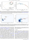 |
Fig. 1 Left: random selection of 200 orbital solutions from the converged part of the MCMC chain. The dashed green and dash-dotted orange ellipses represent the highest-likelihood model from the MCMC chain and the lowest χ2 orbit from the least squares fit, respectively. The blue star marks the location of GG Tau Aa, whereas the dotted ellipse traces the continuum peak intensity along the ring (Andrews et al. 2014; Dutrey et al. 2014). Right: zoom on the region with astrometric coverage. Blue and red points indicate previously published and new astrometric measurements, respectively. The same orbits as in the left panel are rendered. |
 |
Fig. 2 Subset of the parameters describing the GG Tau A orbit: semi-major axis (a), eccentricity (e), and misalignment angle relative to the circumtriple ring (Δθ). In both panels, the blue colour map represent the MCMC posteriors, whereas red dots indicate solutions with |

4.2 Methods
We tuned our initial conditions to reproduce the main characteristics of the GG Tau A system, following the choice in parameters of Cazzoletti et al. (2017) and Aly et al. (2018) (see Table 3 and Fig. 2 for a visualisation of our new astrometric analysis). In particular, the two stars are modelled as sink particles (Bate et al. 1995) with masses of 0.78 M⊙ and 0.68 M⊙. They exert gravitational forces on each other and on the gas and dust particles. In addition, they are subject to the back-reaction force caused by the gas, which ensures the overall conservation of the binary-disc angular momentum. Each of the two sink particles has an associated accretion radius; a radius within which we can consider gas and dust particles to be accreted onto the stars. In particular, we used Rsink = 0.5 AU. We are aware that Rsink is larger than the stars’ radii. Nevertheless, this choice is dictated by the fact that for our purposes we do not need to know what happens to the gas in the vicinity of the stars, so that we can consider gas particles at R < Rsink as accreted. This approximation is not relevant for the dynamical evolution of the dust ring and the gas cavity, but may affect the morphology of the streams of material from the disc to the stars and the formation of inner discs (e.g. Ceppi et al. 2022).
List of parameters. Coplanar 1 and Coplanar 2 differ for the value of Rin, and Misaligned 1 and Misaligned 2 differ for the value of ω(º).
4.3 Initial conditions
The system is surrounded by a disc of 1 × 10⁶ SPH particles, corresponding to a resolved scale height < h > /H of ~0.13– 0.15 for all the simulations. It extends between an inner radius, Rin, which varies in the different configurations (see Table 3 and Sect. 4.4), and an outer radius, Rout = 800 au, and it is centred on the centre of mass of the binary. The surface density distribution is
 (1)
(1)
where R is the radial coordinate in the disc, p =1, and Σ0 is fixed to have a total disc mass of Mg,disc = 0.12 M⊙, as in Guilloteau et al. (1999). For simplicity, we assumed a standard initial dust-to-gas ratio value of e = 10−2, resulting in an initial dust mass of Md,disc = 1.1 × 10⁻³ M⊙, which was assumed to be initially constant throughout the entire disc. This implies that the dust initially has the same vertical structure as the gas, but is allowed to vary during the simulation.
Due to the highly expensive numerical cost of the simulation performed, we fixed a single type of grains with a size of α = 1 mm and an intrinsic density of 3 g cm−3. For the selected set of parameters, the initial mid-plane Stokes number in all the simulations is smaller than unity. This justifies the use of the one fluid algorithm based on the terminal velocity approximation (Laibe & Price 2014; Price & Laibe 2015). Back-reaction from the dust on the gas is automatically included in this approach. We neglected the disc’s self-gravity, as our disc mass results in a gravitationally stable disc.
We assumed a locally isothermal equation of state for the gas, independent of the z for each radius, where the sound speed value, cs, varies as a power law function of the radius with index q = 0.45. We prescribed a radial temperature profile of the form
 (2)
(2)
as has been measured from 13CO observations (e.g. Tang et al. 2016) and fixed in previous numerical studies (Cazzoletti et al. 2017; Aly et al. 2018). Assuming vertical hydrostatic equilibrium, the aspect ratio is
 (3)
(3)
where (H/R)ref = 0.11 at Rref = 100 au to match our disc temperature. For misaligned simulations, the initial misalignment is Δθ = 30º, as in Aly et al. (2018).
We set the value of α SPH artificial viscosity in order to have an effective Shakura & Sunyaev (1973) viscosity of αSS = 0.005. To prevent particle interpenetration, we set the parameter β = 2, as was prescribed in Price (2012). In our initial conditions for the set of simulations, we did not include any circumstellar discs, as their numerical viscous dissipation times are extremely short and they do not affect the evolution of the circumtriple disc4, and their analysis is out of the scope of this paper.
4.4 Simulation set
We ran four SPH simulations with the PHANTOM code, two for the most probable coplanar configuration and two for the most probable misaligned one. Simulations for the same configuration differ in one unconstrained parameter only, to investigate the consequences of different initial conditions. In particular, in the coplanar case, we explored the effect of two different initial conditions for the inner radius of the gas cavity: Rin = [34; 68] AU. In the following, we refer to the simulation with the largest Rin as ‘coplanar 1’ (which exactly replicates the set-up from Cazzoletti et al. 2017), and to the other as ‘coplanar 2’. We note that in the former case, the inner boundary of the disc is equal to the binary semi-major axis, α. According to the work of Ragusa et al. (2020), this distinction in the initial condition can determine a different evolution for the gas over short timescales. Indeed, in their work, the authors find that a smaller initial inner radius leads to the formation of a pronounced, short-lived over-density in the gas surface density.
In the misaligned case, a significant parameter is the argument of periapsis, ω, which measures the mutual inclination between the disc angular momentum, j, and the binary orbital eccentricity, e. The argument of periapsis corresponds to the angle from the body’s ascending node to its periapsis. This parameter is very loosely constrained by observations. Thus, our choice was to perform a set of two simulations, maximising the difference of values for ω = [0º ; 270º] (corresponding to two orthogonal cases of j and e). In the following, we will refer to the simulation with ω = 270º as ‘misaligned 1’ and to the one with ω = 0º as ‘misaligned 2’. In this case, we fixed Rin to 120 AU. The misaligned 1 simulation replicates the best configuration found in Aly et al. (2018).
In Table 3, we summarise the parameters used in our simulations. Each simulation is evolved until the system reaches a steady state. This is ~3000 and ~1500 binary orbits for the copla-nar and misaligned cases, respectively, which both correspond to a physical time of ~5 × 10⁵ yr.
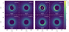 |
Fig. 3 Coplanar simulations, comparison between the initial behaviour shown with the same density and spatial scales. The cyan dots show the position of the binary. Left panels: evolution of the gas surface density in the coplanar 1 simulation for face-on views at different orbital time steps, at 10 (top left), 40 (top right), 80 (bottom left), and 120 (bottom right) Tcopl. The simulation is not forming an over-density in the gas. Right panels: evolution of the gas surface density in the coplanar 2 simulation, at the same times. In both cases, the cavity remains circular. The initial snapshots of coplanar 2 also show how the initial accretion of material around the stars leads to the formation of circumstellar discs, quickly accreted due to low numerical resolution. |
4.5 Radiative transfer and synthetic observations
We post-processed the selected snapshots of all the simulations using MCFOST (Pinte et al. 2006), a Monte Carlo radiative transfer code that maps physical quantities (such as dust density and temperature) directly from the SPH particles using a Voronoi tessellation. The dust distribution in each cell was obtained with a linear interpolation in logarithmic scale of the grain size between 1 µm and 1 mm. Grains larger than 1 mm were assumed to follow the distribution of the 1 mm grains, while the ones smaller than 1 µm were assumed to follow the gas. We assumed a power law grain size distribution of dn/da ∝ a−3.5, with a spanning in a range from amin = 0.03 µm and amax = 3.5 mm. As far as the optical properties were concerned, we used the effective medium theory (EMT) to derive the optical indices of the grains and the Mie theory (spherical and homogeneous dust grains) to compute their absorption and scattering properties. We assumed a chemical composition of 60% silicates, 15% amorphous carbon, and 25% porosity (in volume ratios), as in the DIANA standard dust composition (Woitke et al. 2016). The total gas and dust mass were directly taken from our SPH simulations.
We considered the emission of the two stars as a black-body with effective temperatures of Teff = 4078 K and 3979 K and radii of R★ = 1.55 R⊙ and 1.5 R⊙, respectively, evaluated from the stellar masses according to the isochrones from Siess et al. (2000). In all the simulations, we fixed the distance of the source to d = 145 pc and the inclination of the disc to Δθ = 37º, and we chose a position angle of PA = 97º.
Firstly, we computed the temperature of our models by using 1.3 × 10⁸ photon packets in the Monte Carlo simulation assuming a local thermal equilibrium (LTE). Then, we produced 1300 µm continuum images (corresponding to Band 6 ALMA observations) and 1.67 µm images of the selected snapshots, using the assumption that gas and dust have the same temperature. Finally, in order to generate a synthetic image that can be compared to real observations, we convolved the synthetic images with a Gaussian beam of the same size as the beam of the observations, 0.31″ × 0.15″, PA = 27º for the 1300 µm emission (as in Phuong et al. 2020a) and 0.040" for the 1.67 µm emission (as the PSF value in Keppler et al. 2020), respectively.
5 Results for the coplanar configuration
In the following sections, we show the results of the two different sets of simulations, discussing the dynamical evolution of the systems over short and long timescales (indicatively, <1000 Torb and ≥1000 Torb), and the synthetic images obtained with MCFOST. For the coplanar configuration, the binary period, Tcopl, was used as a time unit. For the chosen parameters, Tcopl corresponds to 1.64 × 10² yr.
5.1 Effect of the initial conditions of the inner edge of the disc
The impact of the different initial conditions of the inner edge of the disc, reproducing the fact that the binary could or could not be initially embedded in the disc, is shown in Fig. 3, where we plot the evolution of the gas surface density for coplanar 1 (top panels) and coplanar 2 (bottom panels) in face-on views at t = 10, 40, 80, 120 Tcopl. In the coplanar 2 case, an over-density forms at the edge of the cavity, precessing with Keplerian velocity, which is not present in the coplanar 1 case. At any rate, this difference is short-lived. Indeed, the two different initial conditions considered eventually lead to the very same stationary configuration (see the bottom right panels of Fig. 3). Therefore, in the following, we consider coplanar 1 as the representative configuration of the coplanar case in general.
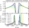 |
Fig. 4 Coplanar 1 simulation, radial cut along the major axis of the gas (top) and dust (bottom) surface density profile as a function of the radial distance from the star, R, up to 3000 Tcopl. After 1500 Tcopl, the eccentricity of the gas cavity starts to grow. As a consequence, the dust ring moves further out. |
5.2 Time evolution
We let the coplanar 1 simulation evolve for ~400 orbits to relax the initial conditions, and then we monitored the dust and gas evolution for ~1000 more orbits, corresponding to ~1.6 × 10⁵ yr. For a visualisation, Fig. 4 shows the evolution of the surface density profiles on a radial cut along the major axis of the gas (top) and dust (bottom). Our findings confirm the prediction that up to 1000 Tcopl the gas is truncated at ~ 80 au, and we find that dust tends to collect at ~ 100–120 au. Following Cazzoletti et al. (2017), we selected the snapshot at 1000 Tcopl as representative of the short timescale behaviour. The disc has a circular cavity, the dust and gas surface density do not show any evident asymmetry and the streams of material appear to be symmetric, as is shown in Fig. 5.
5.3 Long-term evolution
We evolved the coplanar 1 simulations up to 3000 orbital periods (corresponding to ~5 × 10⁵ yr), confirming that long-time evolution processes may change the dust disc size. Indeed, from visual inspection of Fig. 4 we note that the cavity grows in size and eccentricity, and we find that the maximum density moves to larger radii, with dust piling up in an eccentric ring with an apoastron distance of ~200–250 au.
In particular, after 2500 Tcopl (corresponding to ~4.1 × 10⁵ yr), the cavity semi-major axis, a, has grown in size up to a ~ 140 au and it has become eccentric. We find that the dust ring forms at ~200 au, which is closer to its predicted position in the model by Andrews et al. (2014). We note that a prominent over-density, with a contrast ratio of δ ~ 3–45, forms in the gas and dust components, due to the progressive growth in eccentricity. This ‘eccentric feature’ is caused by the clustering of orbits at their apocentres (Ataiee et al. 2013; Teyssandier & Ogilvie 2016).
To quantify these results, we measured the semi-major axis, a, and the eccentricity of the cavity, ecav, in the gas component, using the numerical tool CaSh6. The results are shown in Fig. 6 (for a visualisation of our match with the cavity sizes, see Figs. 5 and 7). For each simulation snapshot, CaSh computes the cavity eccentricity vector and semi-major axis as the average of the SPH particles contained in an interval around Rmid, and the semi-major axis of the inner cavity is defined as the radius, Rmid, at which the surface density becomes half its maximum value (Artymowicz & Lubow 1994). In the following, we also refer to this quantity as the ‘cavity size’.
The cavity remains circular and of the same size (with a radius of ~3 acopl, corresponding to ~100 au) for ~1500 orbits, and then starts to grow in size and becomes increasingly eccentric. At the end of our simulations, after 3500 orbits, the cavity eccentricity has grown up to ~0.4, and the semi-major axis up to ~5 acopl, corresponding to ~170 au. The exact values of these quantities depend on the definition of the surface density threshold for the cavity size7. As the aim of the study is not to perform a study of the growth of ecav in multiple discs, we decided not to evolve the simulation further in order to look for the convergence value, expected to be reached at later times (Ragusa et al. 2018; Hirsh et al. 2020). We adopted the 3000 Tcopl snapshot as representative of the ‘secularly evolved’ scenario, which also takes into account long timescale processes, as it proves the best match to the eccentricity found by Keppler et al. (2020). The cavity size has grown to a ~ 4.5 acopl, with ecav ~ 0.3. The disc features a gas and dust over-density generated by the growth of eccentricity, and asymmetric streams, as is shown in Fig. 7. As a natural consequence of generating an eccentric cavity, the binary’s centre of mass is located in one of the foci.
6 Results for the misaligned configuration
In the following, we use for the misaligned configuration the binary period, Tmis, as time units. For the chosen parameters, Tmis corresponds to 4.3 × 10² yr.
6.1 Effects of the initial value of the binary argument of periapsis
After checking that different initial conditions, once relaxed, do not impact the overall dynamics of the system, we concluded that the two cases evolve towards the same long-timescale behaviour. Indeed, the only difference between the two simulations is the position of the periastron of the system with respect to the chosen reference system, and thus the position of the formation of the eccentric feature (see below). Therefore, in the following, we consider the misaligned 1 configuration to be representative of the misaligned case in general.
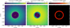 |
Fig. 5 Coplanar 1 simulation: surface density after 1000 orbits, corresponding to ~1.65 × 10⁵ yr. The stars are shown as yellow dots. Left and centre: gas surface density after 1000 orbits (linear and log scales, respectively). Symmetric accretion streams from the disc to the stars can be seen inside the gas cavity. The cavity size obtained with CaSh is over-plotted in red. Right: dust surface density. A circular dusty ring is formed at the location of the gas pressure maximum. No evident asymmetry is visible. |
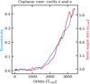 |
Fig. 6 Coplanar 1 simulation: evolution of the cavity semi-major axis, a, expressed in units of the initial semi-major axis of the binary, acopl, and evolution of the eccentricity, ecav, as a function of time measured in Tcopl. After ~2000 orbits, a and ecav start to increase. |
6.2 Time evolution
We let the misaligned 1 simulation evolve for ~200 orbits to relax the initial conditions, and then we monitored the dust and gas evolution for ~600 more orbits (corresponding to ~2.3 × 10⁵ yr). Figure 8 shows the time evolution of the gas and the dust surface density profile for the simulation. In agreement with theoretical and numerical results, the truncation radius (and thus the cavity size) is ~120 au, with a pressure maximum located between 200 and 250 au. The latter corresponds to the position where dust tends to concentrate in our simulations. The gas cavity and the dust ring are also slightly eccentric, with ecav < 0.03, which is hardly noticeable from a visual inspection (see Fig. 9 for the exact value). We selected the 400 Tmis snapshot to represent the ‘standard’ short-timescale behaviour of the misaligned configuration (as in Aly et al. 2018), with an almost circular cavity the size of 3 amis, corresponding to ~180 au, and a symmetric dust ring and streams. The surface density profiles are shown in Fig. 10.
6.3 Long-term evolution
To test how long-time evolution processes also impact the misaligned case, we evolved for the first time the misaligned 1 simulation up to 1500 orbits (corresponding to ~5.8 × 10⁵ yr). During the evolution of the simulation, the value of the inclination of the disc remains almost constant; at the same time, the disc starts to precess around the binary angular momentum.
From Fig. 8, it is clear that, in the misaligned configuration too, the cavity size and eccentricity grow. In particular, after 1500 Tmis (corresponding to ~5.8 × 10⁵ yr), the cavity is larger, ~240 au, and it has become eccentric, with ecav ~ 0.3. As a consequence, the dust ring again becomes wider and more eccentric, developing the eccentric feature with a contrast ratio of δ = 3–4 at the apocentre of the orbits, as in the coplanar case. Figure 9 shows a quantitative analysis of the variation with time of the cavity parameters e and a for the misaligned 1 simulation. We selected the 1500 Tcopl snapshot to represent the ‘secularly evolved’ scenario that is visualised in Fig. 11.
7 Comparison with observations
7.1 Synthetic images
In order to compare our simulations with ALMA and SPHERE observations, we post-processed our representative snapshots to produce synthetic images at 1.67 and 1300 µm. The final gas masses of the two snapshots in the coplanar 1 case are 0.12 M⊙ and 0.11 M⊙, respectively, while the dust mass is ~ 1.2 × 10⁻³ M⊙ for both snapshots. In the misaligned 1 case, the gas masses of the two snapshots are 0.11 M⊙ and 0.095 M⊙, respectively, while the dust mass is ~1.18 × 10⁻³ M⊙. To perform a comparison between different simulations, we decided to fix the dust mass content in the radiative transfer post-process to 10−3 M⊙, a value compatible with the gas mass estimate of the disc and gas-to-dust ratio of 100 (Guilloteau et al. 1999) and with the dust mass estimate from Andrews et al. (2014, ~10−3–10−4 M⊙).
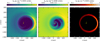 |
Fig. 7 Coplanar 1 simulation: same quantities as Fig. 5 for the longer timescale (3000 orbits), corresponding to ~4.9 × 10⁵ yr. The long-time evolution leads to the growth of eccentricity in the disc. Left and centre: gas surface density after 3000 orbits. Right: dust surface density. The dust is still trapped in the gas pressure maximum in an eccentric ring. |
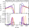 |
Fig. 8 Misaligned 1 case: radial cut along the major axis of the surface density profile of the gas (top, Σg) and dust (bottom, Σd) as a function of the distance of the star, R (au), for different time-steps. Initially, a low-eccentric (ecav ≲ 0.03) cavity and dust ring form. Later on, the simulation shows a larger and more eccentric cavity and dust ring. |
7.2 Observed features
The gas cavity size can be inferred by looking at the 1.67 µm image from Keppler et al. (2020, SPHERE/IRDIS observation, guaranteed-time observations GTO time, project 198.C-0209): assuming that the small dust probed at this wavelength is well coupled with the gas, the size of the cavity in the image is a good estimate of the cavity size of the system.
Likewise, information on the size of the large dust ring comes from the ALMA image of the continuum emission. In this work, we used as a reference the archival ALMA Band 6 observations from Project 2018.1.00532.S (P.I. Denis Alpizar, Otoniel), recently imaged and analysed in Phuong et al. (2020a), calibrated using the ALMA pipeline reduction scripts provided with the raw data from the ALMA archive. Moreover, the model should also show prominent streams of material connecting the inner rim of the cavity to the stars, as was observed in Keppler et al. (2020). Finally, the position of the stars with respect to the centre of the ring is another important signature of an eccentric cavity or ring. Indeed, while for a circular cavity the centre of mass of the binary is located in the centre of the circle, in the case of an elliptic cavity the mass centre of the binary is located in one of the foci. This difference can be in principle hidden due to projection effects, but can be tested in our synthetic images due to the fact that the inclination and position angle of the GG Tau A system have previously been estimated (see Sect. 2). In both observations, the position of the star is central with respect to the gas cavity and the dust ring, but the exact value of the eccentricity of the cavity and dust ring has never been measured. As a rough estimate, as the ‘centre offset’ must be much smaller than the binary separation, e << 0.2. Hereafter, we assume that the cavity is almost circular (i.e. with a low degree of eccentricity).
In Fig. 12, we plot the synthetic images of the representative snapshots for the coplanar (panels a. and b.) and the misaligned (panels c and d) configurations, together with our reference images (top row, panel e, the ALMA Band 6 image, and bottom row, panel e, the 1.67 µm image from Keppler et al. 2020). We also over-plot in grey the 6 and 12 mJy contours of the continuum observation on all the synthetic continuum images. To centre the observed and synthetic images in the same reference system, we used the position of the circumstellar disc of the primary star for the 1300 µm continuum observations, assuming that the primary star is at the centre of its circumstellar disc (top panels), and the estimated position of the stars from the accretion streams of the 1.67 µm image, shown as green crosses, matching the position of the primary star from the observations and from the model8.
Visual inspection of the synthetic and observed 1.67 µm images of the system reveals that our models do no not fully reproduce the SPHERE morphology, with generally too bright and diffuse a northern (front) side. We believe that this indicates that, with our choice of dust opacity, the disc is either too physically thin or too optically thin in the simulations. For this study, or main goal is to match the size of the inner cavity and not to produce a perfect match with all aspects of the ring. We therefore defer to a future work a more quantitative characterisation of the observed features.
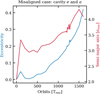 |
Fig. 9 Misaligned 1 simulation: evolution of the cavity semi-major axis, a, and the eccentricity, ecav, as a function of the time, expressed in units of the period of the binary, Tmis. The values of ecav and α increase after ~600 Torb. It should be noted that the initial cavity size jump is due to the stabilisation of the initial conditions. |
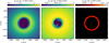 |
Fig. 10 Misaligned 1 simulation: surface density after 400 orbits, corresponding to ~1.54 × 10⁵ yr. The stars are shown as yellow dots. Left and centre: gas surface density after 400 orbits (linear and log scales, respectively). Right: dust surface density. An almost circular dusty ring is formed at the location of the gas pressure maximum, which is larger with respect to the coplanar case size. |
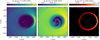 |
Fig. 11 Misaligned 1 simulation: surface density after 1500 orbits, corresponding to ~5.7 × 10⁵ yr. The stars are shown as yellow dots. Left and centre: gas surface density after 1500 orbits. Right: dust surface density. The dust ring is now eccentric. |
7.3 The most likely configuration for GG Tau A
Table 4 shows a visual summary of our analysis. As has been discussed, the phenomenon determining the ‘short’ and ‘long’ timescale evolution in our simulations is the onset of the cavity eccentricity growth in the system, setting a threshold timescale of τecc: the short and long time evolution can then be identified as Torb < τecc or Torb > τecc, respectively, and the system shows different features at different timescales. Focusing on the dust continuum emission (top panels of Fig. 12), we see that the main morphological features are not reproduced in the Coplanar case at either time (Fig. 12 top panels a, b). Moreover, the model predicts a prominent emission asymmetry on the west side of the disc, which is not seen in any of the published results. Inspecting the Misaligned configuration, we can see that the main features are well reproduced for the short-timescale Torb < τecc snapshot (Fig. 12 top panels c), but are no longer a good match for longer timescales. Considering the µm emission (bottom panels of Fig. 12), we find the same trend: the main features of the morphology of the cavity size are only reproduced in the Misaligned case for Torb < τecc. We conclude that the misaligned configuration over short times is the best match of GG Tau A. This is no longer true for longer timescales, Tmis > τecc.
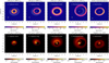 |
Fig. 12 Comparison between the synthetic images at 1300 µm (top) and 1.67 µm (bottom) from the four representative snapshots (two for the coplanar case, a and b, and two for the misaligned case, c and d) and the observed sizes of the dust ring of GG Tau A in Band 6 (see e.g. Phuong et al. 2020a) and gas cavity obtained with SPHERE (Keppler et al. 2020). The stars are shown as cyan dots. The 6 and 12 mJy contours of the continuum observation are over-plotted on the models in grey. In the continuum emission (top), the position of the circumstellar disc detected around GG Tau Aa is also shown, and it is used to centre the observed dust ring on the simulation. In the 1.67 µm images, the positions of the stars in Keppler et al. (2020) are shown as green crosses and are used to centre the observed scattered-light image. |
8 Discussion
Our astrometric and hydrodynamical analysis leads to two main results:
- (1)
The updated astrometric data points and orbital analysis presented here do not allow us to come to any conclusions about the possible coplanarity of the circumtriple ring with the GG Tau Aa-Ab orbit, although a modest degree of misalignment appears likely. To consolidate this result, our multi-wavelength morphological analysis yields the same outcome. This implies that the GG Tau A multiple system is misaligned rather than coplanar. GG Tau A appears to be a typical circum-multiple stellar disc, in which all of the observed discs have a moderate misalignment (neither coplanar nor polar configurations; see e.g. Ceppi et al. 2023, except for the case of very tight binaries that is shown in Czekala et al. 2019). Determining the actual misalignment has an intrinsic value in itself, as several attempts to understand the degree of misalignment between the disc and binary populations and its physical implications have been made (e.g. Czekala et al. 2019).
- (2)
Our results show that the ‘same’ orbital configuration can be ‘observed’ with different morphological characteristics as a result of time evolution, leading to the fact that none of the models is a good match for the observed morphology of the system for all the timescales tested. The fact that disc eccentricity growth appears to be a common phenomenon prompts the question of why the ring is (almost) circular. In the following, we try to answer this question.
8.1 Eccentricity growth: The potential tension between numerical simulations and observations
As has already been discussed in previous sections, eccentricity growth is in agreement with several numerical studies that found that a binary causes the disc eccentricity to grow (e.g. Papaloizou et al. 2001; Kley & Dirksen 2006; MacFadyen & Milosavljević 2008; Shi et al. 2012; Miranda et al. 2017; Muñoz & Lithwick 2020; Ragusa et al. 2020; Pierens et al. 2020; Dittmann & Ryan 2022; Siwek et al. 2023; Franchini et al. 2023), and an overall consensus of binary evolution is found between all the most-used (2D and 3D) numerical codes (Duffell et al. 2024). Consistently with the previous literature, our two representative cases (i.e. coplanar and inclined) both develop cavity eccentricity growth. It is reasonable, then, to assume that other numerical models of this system will show eccentric cavities for ‘most’ choices of the system parameters if sufficiently evolved. How long each phase lasts is hard to know, with the only certainty that most works in the literature suggesting that the final state will be eccentric. For this reason, we simply refer to shorter or longer timescales with respect to the onset of eccentricity growth, τecc.
In light of these considerations, it would be reasonable to expect eccentric circumbinary discs to be common in sufficiently evolved systems. However, this solid numerical result, where all circumbinary discs become eccentric, is somewhat in tension with the few observations available. Detecting the cavity shape of circumbinary discs and obtaining a well-constrained inclination of these discs with respect to the binary orbital plane is a difficult task. Currently, we have well-constrained inclinations of only ten circumbinary discs and nine discs with inclinations measured with moderate uncertainties (Czekala et al. 2019; Ceppi et al. 2023), but disc eccentricity has been measured in only a couple of sources (see below) and a handful of objects have resolved images of the disc, so their eccentricity can be at least visually estimated (six in the sample of Czekala et al. 2019, which explores in total 17 sources).
This small population of circumbinary discs with detected eccentricity (measured or at least visually estimated) consists of nine systems with a range of ages, masses, and different binary orbital parameters; namely, six objects from the sample of Czekala et al. (2019); IRAS 04158+2805 in Ragusa et al. (2021); CS Cha in Kurtovic et al. (2022); GG Tau A in this paper. We find that six objects host almost circular cavities9 and three objects host eccentric (ecav > 0.1) discs10. This implies that the same issue raised in GG Tau A regarding the match between numerical expectations and observations is most likely to occur also when attempting the modelling of other systems characterised by circular cavities.
However, for completeness, we note that sources like IRS 48 (van der Marel et al. 2013; Calcino et al. 2019; Yang et al. 2023) or MWC 758 (Dong et al. 2018; Kuo et al. 2022), hosting eccentric cavities and asymmetric dust emissions, are often put in relationship with binaries, but lack the observational confirmation of the presence of a binary system. On top of that, the source HD142527 (Casassus et al. 2013) exhibits an eccentric cavity and an asymmetric dust ring that can be explained by the presence of a binary (Price et al. 2018a). However, the detected companion appears to be too compact to explain the cavity size and shape (Nowak et al. 2024). In summary, this could possibly improve the statistics of the eccentric circumbinary discs, but would not solve the tension.
We finally note that an eccentric circumbinary disc may evolve in an eccentric planetary system if the disc eccentricity growth is not efficiently dissipated (Bitsch & Kley 2010).
If all the binaries would excite the disc eccentricity growth, we should then expect a higher occurrence of eccentric planets around binary stars. Results from ongoing surveys with ground (e.g. ESPRESSO) and space facilities (e.g. Gaia, TESS) will help us to gauge the extent of these effects.
Table summarising our results from the comparison between GG Tau A models and observations.
8.2 Implications for GG Tau A and other circular circumbinary discs
In order to reconcile the fact that the cavity eccentricity growth appears to be an inevitable consequence in numerical works with the low eccentricity of the dust ring and the cavity observed in the GG Tau A system (but this also applies to other circumbi-nary discs observed to be circular), we identify two possible scenarios, and we discuss their implications:
1. The growth of the cavity eccentricity is common in many cases but it simply does not happen in GG Tau A.
2. The growth of the cavity eccentricity will happen also in GG Tau A, but it has not occurred yet.
In the first scenario, one needs to assume that the growth of the cavity size in eccentric binaries is a common and fast event, occurring for most of the systems on timescales shorter than the disc’s lifetime. This implies that GG Tau A should be a special system. If this is the case, the multiple hierarchy between the components of the GG Tau A,B system may be responsible for damping eccentricity growth. The fact that GG Tau A is not a binary system but a hierarchical triple allows it to excite multiple oscillation modes (see Zanazzi & Lai 2017 or Naoz 2016 for a review, and Ronco et al. 2021 for a specific effect that happens in multiple systems only). However, due to the compact scale of the secondary system, we believe that this effect is not the primary phenomenon responsible for the delaying or damping of the cavity eccentricity growth. Another intriguing explanation may be the presence of a circumtriple planet, located in the cavity, capable of slowing down the disc eccentricity growth (Kurtovic et al. 2022). Currently, no point source has been detected in the cavity; thus, in the case of this system, the presence of an inner planet is not yet supported by observations.
The second scenario deals with the possibility that the GG Tau A disc will become eccentric in the future, but that the timescale for the onset of the cavity eccentricity growth has not been reached yet. This implies either that GG Tau A is a relatively young system if compared with the lifetime of systems hosting eccentric circumbinary discs (~1 Myr) or that the timescale for the eccentricity growth is longer than GG Tau A’s lifetime (~3 Myr, see e.g. White et al. 1999). However, suggesting that the system might be substantially younger would pose a considerable challenge without raising questions about the findings derived from evolutionary models. Therefore, this scenario is unlikely. A more promising way to slow down or damp the eccentricity growth could be the tidal interaction between the primary system GG Tau A, its circumtriple disc, and the secondary system GG Tau B. Indeed, previous studies found that the outer disc of GG Tau A is truncated (Dutrey et al. 1994; Beust & Dutrey 2005), suggesting an efficient removal of material, and thus angular momentum. If this is the case, other excitation modes could be removed, slowing down this kind of process.
By comparing our results for the Coplanar case with Keppler et al. (2020), we see that τecc in the two models, with similar initial conditions but different viscosity values (α = 0.005 and 0.001, respectively), are different by at least a factor of two, with the shorter timescale associated with the higher viscosity. Also, in the literature the value of τecc varies according to the different parameters of the simulations, but eccentricity growth is, as has already been mentioned, always happening. This fact motivates us to speculate that the value of the viscosity plays a relevant role in determining τecc, possibly because viscosity is involved in regulating eccentricity or because it sets the timescale for the response of the system to the variation of its dynamics. If so, its value is such that τecc is so long (or that the growth is so slow) that the disc eccentricity growth will never happen. A lower value of α with respect to the one tested (by at least one order of magnitude) may lead to an increase in τecc, but would also imply that we should not frequently observe very large and eccentric disc cavities. Self-gravitating or cooling effects11 – here completely neglected – may also be relevant in setting the angular momentum transport and the timescales of massive discs (Lodato & Rice 2005). However, as we currently lack a comprehensive understanding of how the actual physical mechanisms responsible for angular momentum transport influence the evolution of the disc’s eccentricity, we might simply not fully understand eccentricity damping mechanisms. It is worth remembering that the α prescription is simply a parametrisation of the disc viscosity.
9 Summary and conclusions
In this work we have analysed the GG Tau A system. We aim to find the best orbital configuration – namely, if the binary-circumtriple disc system is coplanar or misaligned – by combining multi-wavelength information. We present new astro-metric data points from Keck/NIRC2 and VLT/NaCo archival data and we performed an orbital fit, marginally improving the constraints on the orbital parameters. We then devised a suite of four numerical simulations with the 3D SPH hydrodynami-cal code PHANTOM (Price et al. 2018b): two to study the coplanar configuration and two for the misaligned one, using the best configuration from the astrometric fit as the orbital parameters. We tested the dynamical evolution of the two configurations over short and long timescales, and we included for the first time the large dust dynamics.
We showed that, whereas the orbital parameters cannot be determined from astrometry alone due to limited orbital coverage, a morphological analysis is required to obtain relevant information on the most probable orbits. Our main findings regarding GG Tau A are:
We improve on the binary orbital parameters obtained in Köhler (2011) by using a significant extended astromet-ric baseline and by comparing least squares and MCMC approaches to the orbital fit. We find that, despite the fact that the orbital coverage has increased by approximately 50% and all of the newly acquired data points exhibit high precision, the constraints on the orbital parameters have not undergone significant alterations when using the same least squares orbital fitting method. However, the MCMC approach shows that the lowest χ2 solutions are also much less plausible statistically speaking, highlighting the importance of priors in the fit and the need for an even longer baseline to make significant progress in constraining the orbit. All things considered, it appears likely, though not certain, that the ring is modestly misaligned with the orbit, and that it has a low eccentricity.
For each configuration, we studied the effect of the initial condition – namely, the initial cavity size for the copla-nar configuration and the mutual inclination between the angular momentum of the binary and the cavity for the misaligned configuration – showing that those parameters do not influence the global evolution of the simulation.
We find that the coplanar configuration on short timescales has a cavity size and a dust ring size that are too small with respect to the observed ones. Instead, over longer timescales, this configuration leads to a larger and eccentric gas cavity with prominent accretion streams. However, it still fails to reproduce the basic observed features (cavity size and dust ring size).
The misaligned configuration over shorter timescales is able to reproduce all of the observed features of GG Tau A without requiring a highly eccentric gas cavity. We thus conclude that the most probable configuration for the GG Tau A system is a modestly misaligned configuration with a binary-semi-major axis of amis ~ 50–60 au, an eccentricity of e ~ 0.1–0.4, and Δθ ~ 10º–30º.
Over longer timescales, once the cavity eccentricity growth modes are excited, the misaligned configuration also fails to reproduce the observations, as the gas cavity becomes too large and too eccentric. Such a fast growth in the binary eccentricity is at odds with the age of the system.
The last result implies that: (i) the timescale for the onset of the eccentricity growth, τecc, is a fundamental timescale for the system evolution; (ii) τecc is longer than the age of the system; or (iii) there are physical mechanisms playing a role in the disc eccentricity evolution that we are not considering. Due to the specific hierarchical configuration of the system, the tidal interaction between the GG Tau A circumtriple disc and the GG Tau B binary system (which is known to determine the outer disc truncation) may be responsible for slowing down the eccentricity growth.
In a broader context, our findings prompt us to consider if the onset of the eccentricity growth is a common process in observed binary systems, critically impacting their morphology and the architecture of the eventual hosted planetary systems. Eccentric cavities could be frequent and dust can potentially be trapped in the resulting over-density. This would lead to the formation of planets in eccentric circumtriple orbits. Moreover, as the binary in an eccentric cavity is located in one of the foci, this gives stringent constraints on the observational signatures of a binary in an eccentric disc. Ongoing and future surveys will be key to better constraining the population of eccentric discs and exoplanets in multiple stellar systems.
Acknowledgements
We thank the anonymous Referee for the useful suggestions. CT thanks Francesco Zagaria and Nicolas T. Kurtovic for the insightful scientific discussions and the valuable support. This project has received funding from the European Union’s Horizon 2020 research and innovation programme under the Marie Sklodowska Curie grant agreement no. 823823 (DUSTBUSTERS RISE project). This project has received funding from the European Research Council (ERC) under the European Union Horizon Europe programme (grant agreement no. 101042275, project Stellar-MADE). This project has received funding from the European Research Council (ERC) under the European Union’s Horizon Europe research and innovation program (grant agreement no. 101053020, project Dust2Planets). E.R. acknowledges financial support from the European Union’s Horizon Europe research and innovation programme under the Marie Skłodowska-Curie grant agreement no. 101102964 (ORBIT-D). E.R. also acknowledges financial support from the European Research Council (ERC) under the European Union’s Horizon 2020 research and innovation programme (grant agreement no. 864965, PODCAST). H.A. acknowledges funding from the European Research Council (ERC) under the European Union’s Horizon 2020 research and innovation programme (grant agreement no. 101054502). This research has made use of the Keck Observatory Archive (KOA), which is operated by the W. M. Keck Observatory and the NASA Exoplanet Science Institute (NExScI), under contract with the National Aeronautics and Space Administration. This paper makes use of the following ALMA data: ADS/JAO.ALMA 2018.1.00532.S ALMA is a partnership of ESO (representing its member states), NSF (USA) and NINS (Japan), together with NRC (Canada), MOST and ASIAA (Taiwan), and KASI (Republic of Korea), in cooperation with the Republic of Chile. The Joint ALMA Observatory is operated by ESO, AUI/NRAO and NAOJ. In addition, publications from NA authors must include the standard NRAO acknowledgement: The National Radio Astronomy Observatory is a facility of the National Science Foundation operated under cooperative agreement by Associated Universities, Inc. This paper uses the following Python libraries: Numpy, Matplotlib, Astropy, Scipy, Glob, and the following visualization tools: pymcfost, plonk.
Appendix A Orbital fit: Markov-Chain Monte Carlo corner plot
In Figure A.1, we present the full corner plot obtained using orbitize! to fit the orbit of the GG Tau A system.
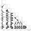 |
Fig. A.1 Corner plot resulting from the orbitize! fit to the GG Tau A orbit. |
References
- Aly, H., Lodato, G., & Cazzoletti, P. 2018, MNRAS, 480, 4738 [NASA ADS] [Google Scholar]
- Andrews, S. M., Chandler, C. J., Isella, A., et al. 2014, ApJ, 787, 148 [NASA ADS] [CrossRef] [Google Scholar]
- Artymowicz, P., & Lubow, S. H. 1994, ApJ, 421, 651 [Google Scholar]
- Ataiee, S., Pinilla, P., Zsom, A., et al. 2013, A&A, 553, A3 [Google Scholar]
- Bate, M. R. 1998, ApJ, 508, L95 [NASA ADS] [CrossRef] [Google Scholar]
- Bate, M. R. 2018, MNRAS, 475, 5618 [Google Scholar]
- Bate, M. R., Bonnell, I. A., & Price, N. M. 1995, MNRAS, 277, 362 [Google Scholar]
- Beust, H., & Dutrey, A. 2005, A&A, 439, 585 [NASA ADS] [CrossRef] [EDP Sciences] [Google Scholar]
- Bitsch, B., & Kley, W. 2010, A&A, 523, A30 [NASA ADS] [CrossRef] [EDP Sciences] [Google Scholar]
- Blunt, S., Wang, J. J., Angelo, I., et al. 2020, AJ, 159, 89 [NASA ADS] [CrossRef] [Google Scholar]
- Calcino, J., Price, D. J., Pinte, C., et al. 2019, MNRAS, 490, 2579 [Google Scholar]
- Casassus, S., van der Plas, G. M., Perez, S., et al. 2013, Nature, 493, 191 [Google Scholar]
- Cazzoletti, P., Ricci, L., Birnstiel, T., & Lodato, G. 2017, A&A, 599, A102 [NASA ADS] [CrossRef] [EDP Sciences] [Google Scholar]
- Ceppi, S., Cuello, N., Lodato, G., et al. 2022, MNRAS, 514, 906 [CrossRef] [Google Scholar]
- Ceppi, S., Longarini, C., Lodato, G., Cuello, N., & Lubow, S. H. 2023, MNRAS, 520, 5817 [NASA ADS] [CrossRef] [Google Scholar]
- Chen, X., Arce, H. G., Zhang, Q., et al. 2013, ApJ, 768, 110 [Google Scholar]
- Clarke, C. J., Bonnell, I. A., & Hillenbrand, L. A. 2000, in Protostars and Planets IV, eds. V. Mannings, A. P. Boss, & S. S. Russell, 151 [Google Scholar]
- Czekala, I., Chiang, E., Andrews, S. M., et al. 2019, ApJ, 883, 22 [NASA ADS] [CrossRef] [Google Scholar]
- D’Angelo, G., Lubow, S. H., & Bate, M. R. 2006, ApJ, 652, 1698 [CrossRef] [Google Scholar]
- Di Folco, E., Dutrey, A., Le Bouquin, J. B., et al. 2014, A&A, 565, A2 [Google Scholar]
- Dittmann, A. J., & Ryan, G. 2022, MNRAS, 513, 6158 [NASA ADS] [Google Scholar]
- Dong, R., Liu, S.-y., Eisner, J., et al. 2018, ApJ, 860, 124 [Google Scholar]
- D’Orazio, D. J., & Duffell, P. C. 2021, ApJ, 914, L21 [CrossRef] [Google Scholar]
- Doyle, L. R., Carter, J. A., Fabrycky, D. C., et al. 2011, Science, 333, 1602 [NASA ADS] [CrossRef] [Google Scholar]
- Duchêne, G., & Kraus, A. 2013, ARA&A, 51, 269 [Google Scholar]
- Duchene, G., McCabe, C., Ghez, A., & Macintosh, B. 2004, ApJ, 606, 969 [NASA ADS] [CrossRef] [Google Scholar]
- Duchêne, G., LeBouquin, J.-B., Ménard, F., et al. 2024, A&A, 686, A188 [NASA ADS] [CrossRef] [EDP Sciences] [Google Scholar]
- Duffell, P. C., Dittmann, A. J., D’Orazio, D. J., et al. 2024, arXiv e-prints [arXiv:2402.13039] [Google Scholar]
- Dutrey, A., Guilloteau, S., & Simon, M. 1994, A&A, 286, 149 [NASA ADS] [Google Scholar]
- Dutrey, A., di Folco, E., Guilloteau, S., et al. 2014, Nature, 514, 600 [NASA ADS] [CrossRef] [Google Scholar]
- Franchini, A., Lupi, A., Sesana, A., & Haiman, Z. 2023, MNRAS, 522, 1569 [NASA ADS] [CrossRef] [Google Scholar]
- Gaia Collaboration (Prusti, T., et al.) 2016, A&A, 595, A1 [NASA ADS] [CrossRef] [EDP Sciences] [Google Scholar]
- Gaia Collaboration (Vallenari, A., et al.) 2023, A&A, 674, A1 [NASA ADS] [CrossRef] [EDP Sciences] [Google Scholar]
- Galli, P. A. B., Loinard, L., Bouy, H., et al. 2019, A&A, 630, A137 [NASA ADS] [CrossRef] [EDP Sciences] [Google Scholar]
- Guilloteau, S., Dutrey, A., & Simon, M. 1999, A&A, 348, 570 [NASA ADS] [Google Scholar]
- Hartkopf, W. I., McAlister, H. A., & Franz, O. G. 1989, AJ, 98, 1014 [NASA ADS] [CrossRef] [Google Scholar]
- Hirsh, K., Price, D. J., Gonzalez, J.-F., Ubeira-Gabellini, M. G., & Ragusa, E. 2020, MNRAS, 498, 2936 [NASA ADS] [CrossRef] [Google Scholar]
- Horch, E. P., Broderick, K. G., Casetti-Dinescu, D. I., et al. 2021, AJ, 161, 295 [NASA ADS] [CrossRef] [Google Scholar]
- Kennedy, G. M., Matrà, L., Facchini, S., et al. 2019, Nat. Astron., 3, 230 [Google Scholar]
- Keppler, M., Penzlin, A., Benisty, M., et al. 2020, A&A, 639, A62 [NASA ADS] [CrossRef] [EDP Sciences] [Google Scholar]
- Kley, W., & Dirksen, G. 2006, A&A, 447, 369 [NASA ADS] [CrossRef] [EDP Sciences] [Google Scholar]
- Köhler, R. 2011, A&A, 530, A126 [NASA ADS] [CrossRef] [EDP Sciences] [Google Scholar]
- Kraus, A. L., & Hillenbrand, L. A. 2009, ApJ, 704, 531 [Google Scholar]
- Krist, J. E., Stapelfeldt, K. R., & Watson, A. M. 2002, ApJ, 570, 785 [NASA ADS] [CrossRef] [Google Scholar]
- Kuo, I. H. G., Yen, H.-W., Gu, P.-G., & Chang, T.-E. 2022, ApJ, 938, 50 [NASA ADS] [CrossRef] [Google Scholar]
- Kurtovic, N. T., Pinilla, P., Penzlin, A. B. T., et al. 2022, A&A, 664, A151 [NASA ADS] [CrossRef] [EDP Sciences] [Google Scholar]
- Laibe, G., & Price, D. J. 2014, MNRAS, 440, 2136 [Google Scholar]
- Leinert, C., Haas, M., Mundt, R., Richichi, A., & Zinnecker, H. 1991, A&A, 250, 407 [NASA ADS] [Google Scholar]
- Leinert, C., Zinnecker, H., Weitzel, N., et al. 1993, A&A, 278, 129 [NASA ADS] [Google Scholar]
- Lester, K. V., Schaefer, G. H., Fekel, F. C., et al. 2022, AJ, 164, 228 [NASA ADS] [CrossRef] [Google Scholar]
- Lodato, G., & Rice, W. K. M. 2005, MNRAS, 358, 1489 [Google Scholar]
- Luhman, K. L. 1999, ApJ, 525, 466 [Google Scholar]
- MacFadyen, A. I., & Milosavljevic, M. 2008, ApJ, 672, 83 [NASA ADS] [CrossRef] [Google Scholar]
- Manara, C., Tazzari, M., Long, F., et al. 2019, A&A, 628, A95 [NASA ADS] [CrossRef] [EDP Sciences] [Google Scholar]
- Martin, D. V. 2018, in Handbook of Exoplanets, eds. H. J. Deeg, & J. A. Belmonte, 156 [Google Scholar]
- Mason, B. D., Douglass, G. G., & Hartkopf, W. I. 1999, AJ, 117, 1023 [NASA ADS] [CrossRef] [Google Scholar]
- Miranda, R., Muñoz, D. J., & Lai, D. 2017, MNRAS, 466, 1170 [NASA ADS] [CrossRef] [Google Scholar]
- Moe, M., & Kratter, K. M. 2021, MNRAS, 507, 3593 [NASA ADS] [CrossRef] [Google Scholar]
- Muñoz, D. J., & Lithwick, Y. 2020, ApJ, 905, 106 [CrossRef] [Google Scholar]
- Naoz, S. 2016, ARA&A, 54, 441 [Google Scholar]
- Nelson, A. F., & Marzari, F. 2016, ApJ, 827, 93 [Google Scholar]
- Nowak, M., Rowther, S., Lacour, S., et al. 2024, A&A, 683, A6 [NASA ADS] [CrossRef] [EDP Sciences] [Google Scholar]
- Offner, S. S. R., Moe, M., Kratter, K. M., et al. 2023, Protostars and Planets VII, ed. S. Inutsuka, Y. Aikawa, T. Muto, K. Tomida, and M. Tamura. ASP Conf. Ser., 534, 275 [NASA ADS] [Google Scholar]
- Ogilvie, G., & Lubow, S. H. 2003, ApJ, 587, 398 [NASA ADS] [CrossRef] [Google Scholar]
- Papaloizou, J., Nelson, R. P., & Masset, F. 2001, A&A, 366, 263 [NASA ADS] [CrossRef] [EDP Sciences] [Google Scholar]
- Phuong, N. T., Dutrey, A., Di Folco, E., et al. 2020a, A&A, 635, A9 [EDP Sciences] [Google Scholar]
- Phuong, N. T., Dutrey, A., Diep, P. N., et al. 2020b, A&A, 635, A12 [NASA ADS] [CrossRef] [EDP Sciences] [Google Scholar]
- Phuong, N. T., Dutrey, A., Chapillon, E., et al. 2021, A&A, 653, A5 [NASA ADS] [CrossRef] [EDP Sciences] [Google Scholar]
- Pierens, A., McNally, C. P., & Nelson, R. P. 2020, MNRAS, 496, 2849 [CrossRef] [Google Scholar]
- Pinilla, P., Birnstiel, T., Ricci, L., et al. 2012, A&A, 538, A114 [NASA ADS] [CrossRef] [EDP Sciences] [Google Scholar]
- Pinte, C., Ménard, F., Duchêne, G., & Bastien, P. 2006, A&A, 459, 797 [NASA ADS] [CrossRef] [EDP Sciences] [Google Scholar]
- Poblete, P. P., Cuello, N., & Cuadra, J. 2019, MNRAS, 489, 2204 [NASA ADS] [CrossRef] [Google Scholar]
- Price, D. J. 2012, J. Comput. Phys., 231, 759 [NASA ADS] [CrossRef] [Google Scholar]
- Price, D. J., & Laibe, G. 2015, MNRAS, 451, 813 [NASA ADS] [CrossRef] [Google Scholar]
- Price, D. J., Cuello, N., Pinte, C., et al. 2018a, MNRAS, 477, 1270 [Google Scholar]
- Price, D. J., Wurster, J., Tricco, T. S., et al. 2018b, PASA, 35, e031 [Google Scholar]
- Ragusa, E., Dipierro, G., Lodato, G., Laibe, G., & Price, D. J. 2017, MNRAS, 464, 1449 [Google Scholar]
- Ragusa, E., Rosotti, G., Teyssandier, J., et al. 2018, MNRAS, 474, 4460 [CrossRef] [Google Scholar]
- Ragusa, E., Alexander, R., Calcino, J., Hirsh, K., & Price, D. J. 2020, MNRAS, 499, 3362 [NASA ADS] [CrossRef] [Google Scholar]
- Ragusa, E., Fasano, D., Toci, C., et al. 2021, MNRAS, 507, 1157 [NASA ADS] [CrossRef] [Google Scholar]
- Ronco, M. P., Guilera, O. M., Cuadra, J., et al. 2021, ApJ, 916, 113 [NASA ADS] [CrossRef] [Google Scholar]
- Rota, A. A., Meijerhof, J. D., van der Marel, N., et al. 2024, A&A, 684, A134 [NASA ADS] [CrossRef] [EDP Sciences] [Google Scholar]
- Schaefer, G. H., Simon, M., Beck, T. L., Nelan, E., & Prato, L. 2006, AJ, 132, 2618 [NASA ADS] [CrossRef] [Google Scholar]
- Shakura, N., & Sunyaev, R. 1973, in IAU Symp., 55, X- and Gamma-Ray Astronomy, eds. H. Bradt, & R. Giacconi, 155 [Google Scholar]
- Shi, J.-M., Krolik, J. H., Lubow, S. H., & Hawley, J. F. 2012, ApJ, 749, 118 [Google Scholar]
- Siess, L., Dufour, E., & Forestini, M. 2000, A&A, 358, 593 [Google Scholar]
- Silber, J., Gledhill, T., Duchêne, G., & Ménard, F. 2000, ApJ, 536, L89 [Google Scholar]
- Siwek, M., Weinberger, R., Muñoz, D. J., & Hernquist, L. 2023, MNRAS, 518, 5059 [Google Scholar]
- Standing, M. R., Sairam, L., Martin, D. V., et al. 2023, Nature, 7, 702 [NASA ADS] [Google Scholar]
- Tang, Y.-W., Dutrey, A., Guilloteau, S., et al. 2016, ApJ, 820, 19 [NASA ADS] [CrossRef] [Google Scholar]
- Tang, Y.-W., Dutrey, A., Koch, P. M., et al. 2023, ApJ, 947, L5 [NASA ADS] [CrossRef] [Google Scholar]
- Teyssandier, J., & Ogilvie, G. I. 2016, MNRAS, 458, 3221 [NASA ADS] [CrossRef] [Google Scholar]
- Thun, D., Kley, W., & Picogna, G. 2017, A&A, 604, A102 [NASA ADS] [CrossRef] [EDP Sciences] [Google Scholar]
- Tobin, J. J., Looney, L. W., Li, Z.-Y., et al. 2016, ApJ, 818, 73 [CrossRef] [Google Scholar]
- Tokovinin, A., Mason, B. D., Mendez, R. A., & Costa, E. 2022, AJ, 164, 58 [NASA ADS] [CrossRef] [Google Scholar]
- Toonen, S., Hamers, A., & Portegies Zwart, S. 2016, Comput. Astrophys. Cosmol., 3, 6 [NASA ADS] [CrossRef] [Google Scholar]
- van der Marel, N., van Dishoeck, E. F., Bruderer, S., et al. 2013, Science, 340, 1199 [Google Scholar]
- Vousden, W. D., Farr, W. M., & Mandel, I. 2016, MNRAS, 455, 1919 [NASA ADS] [CrossRef] [Google Scholar]
- White, R. J., & Ghez, A. M. 2001, ApJ, 556, 265 [Google Scholar]
- White, R. J., Ghez, A. M., Reid, I. N., & Schultz, G. 1999, ApJ, 520, 811 [NASA ADS] [CrossRef] [Google Scholar]
- Woitke, P., Min, M., Pinte, C., et al. 2016, A&A, 586, A103 [NASA ADS] [CrossRef] [EDP Sciences] [Google Scholar]
- Yang, H., Fernández-López, M., Li, Z.-Y., et al. 2023, ApJ, 948, L2 [NASA ADS] [CrossRef] [Google Scholar]
- Zagaria, F., Rosotti, G. P., Alexander, R. D., & Clarke, C. J. 2023, Eur. Phys. J. Plus, 138, 25 [NASA ADS] [CrossRef] [Google Scholar]
- Zanazzi, J. J., & Lai, D. 2017, MNRAS, 467, 1957 [Google Scholar]
- Zurlo, A., Gratton, R., Pérez, S., & Cieza, L. 2023, Eur. Phys. J. Plus, 138, 411 [NASA ADS] [CrossRef] [Google Scholar]
i.e. a triple system consisting of an inner binary and an outer star, where the centre of mass can be closer to the inner binary or the outer star; for a review of the evolution of hierarchical stellar systems see e.g. Toonen et al. (2016).
The total angular momentum of the system is highly dominated by the angular momentum of the Aa–Ab pair, the effects produced by the binarity of Ab1–Ab2 appear only on secular timescales as perturbations to the Aa–Ab system on the disc.
Where δ is defined as the ratio between the density in the azimuthal feature and the density at the opposite side of the cavity.
CaSh is available at the following Github repository https://github.com/si-mon-jinn/CaSh
Note that in this work, following Artymowicz & Lubow (1994), the threshold for the surface density is 50% of the peak value, while in Keppler et al. (2020) the threshold value is the 10% of the peak value. However, results are similar for the different thresholds.
The exact position of the secondary star may differ in each simulation, as it depends from the phase of the binary orbit and the relative inclination between the plane of the sky and the orbital planes.
V4046, AK Sco, DQ Tau, HD98800 B, GG Tau A, CS Cha, with 4 coplanar, 1 misaligned and one polar systems.
GW Ori AB, HD142527, IRAS 04158+2805, all misaligned (and one triple system, GW Ori).
As a higher cooling factor sets a decreasing of the thermal velocity of particles.
All Tables
List of parameters. Coplanar 1 and Coplanar 2 differ for the value of Rin, and Misaligned 1 and Misaligned 2 differ for the value of ω(º).
Table summarising our results from the comparison between GG Tau A models and observations.
All Figures
|
Fig. 1 Left: random selection of 200 orbital solutions from the converged part of the MCMC chain. The dashed green and dash-dotted orange ellipses represent the highest-likelihood model from the MCMC chain and the lowest χ2 orbit from the least squares fit, respectively. The blue star marks the location of GG Tau Aa, whereas the dotted ellipse traces the continuum peak intensity along the ring (Andrews et al. 2014; Dutrey et al. 2014). Right: zoom on the region with astrometric coverage. Blue and red points indicate previously published and new astrometric measurements, respectively. The same orbits as in the left panel are rendered. |
| In the text | |
|
Fig. 2 Subset of the parameters describing the GG Tau A orbit: semi-major axis (a), eccentricity (e), and misalignment angle relative to the circumtriple ring (Δθ). In both panels, the blue colour map represent the MCMC posteriors, whereas red dots indicate solutions with |
| In the text | |
|
Fig. 3 Coplanar simulations, comparison between the initial behaviour shown with the same density and spatial scales. The cyan dots show the position of the binary. Left panels: evolution of the gas surface density in the coplanar 1 simulation for face-on views at different orbital time steps, at 10 (top left), 40 (top right), 80 (bottom left), and 120 (bottom right) Tcopl. The simulation is not forming an over-density in the gas. Right panels: evolution of the gas surface density in the coplanar 2 simulation, at the same times. In both cases, the cavity remains circular. The initial snapshots of coplanar 2 also show how the initial accretion of material around the stars leads to the formation of circumstellar discs, quickly accreted due to low numerical resolution. |
| In the text | |
|
Fig. 4 Coplanar 1 simulation, radial cut along the major axis of the gas (top) and dust (bottom) surface density profile as a function of the radial distance from the star, R, up to 3000 Tcopl. After 1500 Tcopl, the eccentricity of the gas cavity starts to grow. As a consequence, the dust ring moves further out. |
| In the text | |
|
Fig. 5 Coplanar 1 simulation: surface density after 1000 orbits, corresponding to ~1.65 × 10⁵ yr. The stars are shown as yellow dots. Left and centre: gas surface density after 1000 orbits (linear and log scales, respectively). Symmetric accretion streams from the disc to the stars can be seen inside the gas cavity. The cavity size obtained with CaSh is over-plotted in red. Right: dust surface density. A circular dusty ring is formed at the location of the gas pressure maximum. No evident asymmetry is visible. |
| In the text | |
|
Fig. 6 Coplanar 1 simulation: evolution of the cavity semi-major axis, a, expressed in units of the initial semi-major axis of the binary, acopl, and evolution of the eccentricity, ecav, as a function of time measured in Tcopl. After ~2000 orbits, a and ecav start to increase. |
| In the text | |
|
Fig. 7 Coplanar 1 simulation: same quantities as Fig. 5 for the longer timescale (3000 orbits), corresponding to ~4.9 × 10⁵ yr. The long-time evolution leads to the growth of eccentricity in the disc. Left and centre: gas surface density after 3000 orbits. Right: dust surface density. The dust is still trapped in the gas pressure maximum in an eccentric ring. |
| In the text | |
|
Fig. 8 Misaligned 1 case: radial cut along the major axis of the surface density profile of the gas (top, Σg) and dust (bottom, Σd) as a function of the distance of the star, R (au), for different time-steps. Initially, a low-eccentric (ecav ≲ 0.03) cavity and dust ring form. Later on, the simulation shows a larger and more eccentric cavity and dust ring. |
| In the text | |
|
Fig. 9 Misaligned 1 simulation: evolution of the cavity semi-major axis, a, and the eccentricity, ecav, as a function of the time, expressed in units of the period of the binary, Tmis. The values of ecav and α increase after ~600 Torb. It should be noted that the initial cavity size jump is due to the stabilisation of the initial conditions. |
| In the text | |
|
Fig. 10 Misaligned 1 simulation: surface density after 400 orbits, corresponding to ~1.54 × 10⁵ yr. The stars are shown as yellow dots. Left and centre: gas surface density after 400 orbits (linear and log scales, respectively). Right: dust surface density. An almost circular dusty ring is formed at the location of the gas pressure maximum, which is larger with respect to the coplanar case size. |
| In the text | |
|
Fig. 11 Misaligned 1 simulation: surface density after 1500 orbits, corresponding to ~5.7 × 10⁵ yr. The stars are shown as yellow dots. Left and centre: gas surface density after 1500 orbits. Right: dust surface density. The dust ring is now eccentric. |
| In the text | |
|
Fig. 12 Comparison between the synthetic images at 1300 µm (top) and 1.67 µm (bottom) from the four representative snapshots (two for the coplanar case, a and b, and two for the misaligned case, c and d) and the observed sizes of the dust ring of GG Tau A in Band 6 (see e.g. Phuong et al. 2020a) and gas cavity obtained with SPHERE (Keppler et al. 2020). The stars are shown as cyan dots. The 6 and 12 mJy contours of the continuum observation are over-plotted on the models in grey. In the continuum emission (top), the position of the circumstellar disc detected around GG Tau Aa is also shown, and it is used to centre the observed dust ring on the simulation. In the 1.67 µm images, the positions of the stars in Keppler et al. (2020) are shown as green crosses and are used to centre the observed scattered-light image. |
| In the text | |
|
Fig. A.1 Corner plot resulting from the orbitize! fit to the GG Tau A orbit. |
| In the text | |
Current usage metrics show cumulative count of Article Views (full-text article views including HTML views, PDF and ePub downloads, according to the available data) and Abstracts Views on Vision4Press platform.
Data correspond to usage on the plateform after 2015. The current usage metrics is available 48-96 hours after online publication and is updated daily on week days.
Initial download of the metrics may take a while.