| Issue |
A&A
Volume 685, May 2024
|
|
|---|---|---|
| Article Number | A35 | |
| Number of page(s) | 14 | |
| Section | Planets and planetary systems | |
| DOI | https://doi.org/10.1051/0004-6361/202348347 | |
| Published online | 03 May 2024 | |
Study of type II migration under the framework of the disk instability model for giant planet formation
College of Physics, Jilin University,
Changchun,
Jilin
130012,
PR China
e-mail: jinlp@jlu.edu.cn; jingxi16@mails.jlu.edu.cn
Received:
22
October
2023
Accepted:
20
February
2024
Context. Hydrodynamic simulations of the migration of planets formed by gravitational instability suggest that after an initial phase of fast migration, planets can open gaps and continue to migrate on a type II migration timescale. The simulation time length is typically on the order of 104 yr.
Aims. We study the effects of the subsequent type II migration during the disk lifetime on the final orbital radii of planets.
Methods. We used a numerical disk model that follows the disk formation and evolution. The disk acquires mass through the mass influx from the collapse of its parent molecular cloud core. The model reflects the influence of the properties of the parent core on the disk. Considering clumps forming at different times in a disk and also in different disks with different parent core properties, we used the type II migration rate to follow the clump migration from the formation location. We studied the dependence of the clump migration on the properties of the parent core.
Results. The mass influx drag enhances the migration process. The duration and viscosity of gravitational instability, viscosity in the dead zone, and the collapse time of the parent core play important roles in planet migration. As the angular momentum and mass of the parent core increase, migration is enhanced. The final radius is sensitive to the initial radius. Clumps forming at large radii might migrate outward with the disk expansion.
Conclusions. Even though type II migration is slow, clumps can migrate over significant distances. A considerable proportion of clumps migrate to the central protostar via type II migration. Our calculations support the idea that the observed pile-up of planets at <0.3 AU is explained by a scenario where planets might form at large radii, then migrate to orbits of <0.3 AU, and halt by a stopping mechanism at this location.
Key words: planets and satellites: formation / protoplanetary disks / planet–disk interactions / planetary systems
© The Authors 2024
 Open Access article, published by EDP Sciences, under the terms of the Creative Commons Attribution License (https://creativecommons.org/licenses/by/4.0), which permits unrestricted use, distribution, and reproduction in any medium, provided the original work is properly cited.
This article is published in open access under the Subscribe to Open model. Subscribe to A&A to support open access publication.
1 Introduction
Significant progress in the observation of exoplanets has been made thanks to the launch of Kepler and TESS. A large number of data on exoplanet properties, such as the semi-major axis, mass, radius, and eccentricity, have been collected1 (e.g., Zhu & Dong 2021). However, theoretical calculations of planet formation are still far from precisely matching what has been seen in the observational data. From a molecular cloud core to the final planetary system, the system goes through numerous physical processes. These processes are so complex that it is a challenge to quantitatively treat them and link these processes together to get a whole quantitative picture. There are many uncertainties in this field and one of the unknowns in the theory of planet formation is the effect of planet migration. To understand observed semi-major axes, it seems to us that migration must be understood quantitatively. A substantial amount of work has been devoted to the topic of migration (for a review of migration, see, e.g., Baruteau et al. 2014; Paardekooper et al. 2023). One of the more outstanding observations is that a large number of planets pile up at semi-major axes lower than 0.3 AU. One possible scenario posits a planet might form at a large radius, then migrate to an orbit of <0.3 AU, and be halted there by a stopping mechanism (Lin et al. 1996; Trilling et al. 1998; Miranda & Lai 2018; Romanova et al. 2019; Flock et al. 2019; Paardekooper et al. 2023, Sect. 3.8). Therefore, migration may play a critical role in making planets gather on orbits of <0.3 AU. For a recent review on stopping mechanism and migration near the inner disk edge, we refer to Sect. 3.8 of Paardekooper et al. (2023).
For giant planet formation, two theories have been proposed: the core accretion model and the disk instability model (for reviews, see, e.g., Armitage 2010; D’Angelo et al. 2011; Helled et al. 2014; Drążkowska et al. 2023). In the disk instability model, a gravitationally unstable disk fragments into dense self-gravitating clumps. They then contract to form gas giant planets. We note that clumps can form only in the fragmentation region if they can form at all. In this paper, we mainly focus on the type II migration of clumps and their final migration destinies under the framework of the disk instability model. For a recent review of the specific topic on the migration of clumps formed by gravitational instability, we refer to Sect. 3.7 of Paardekooper et al. (2023).
The interaction between a planet and its nascent disk can change the planet’s orbital radius, causing it to migrate (Lin & Papaloizou 1979; Goldreich & Tremaine 1980). It is thought that a planet more massive than Saturn can open a gap around its orbit (e.g., Armitage 2010). Lin & Papaloizou (1986b) investigated the tidal interaction between a protoplanetary disk and a protoplanet and the orbital migration of the protoplanet. They found that if a protoplanet is initially found at small radii, it migrates inward; whereas if it is initially at large radii, it migrates outward. For intermediate initial radii, a protoplanet migrates outward first and then inward.
Ward (1997) proposed an analytical model that shows two types of protoplanet migration. In the first type, a protoplanet migrates in the disk because of torque asymmetries. This author found that the migration rate is proportional to the disk surface density and to the protoplanet mass. In the second type, the protoplanet is locked to the disk due to the gap formation.
Veras & Armitage (2004) studied planet migration in an evolving disk and found that the planet migration can be outward in the part where the gas disk expands. These authors showed the possibility that there is a region in the disk where the gas radial velocity is outward, which can drive substantial outward migration.
Zhu et al. (2012) used 2D hydrodynamic simulations of protoplanetary disks to study disk gravitational instability and fragmentation, as well as the clump formation and migration. These authors simulated the disk stage near the end of the collapse of the parent molecular cloud core. In their simulations, the final fates of these formed clumps vary: among 13 clumps, 3 are massive enough (in the mass range of brown dwarfs) to open gaps and to basically stop migrating; 4 clumps are disrupted tidally in the process of inward migration; and 6 clumps migrate through the inner boundary of their modeled disks. Vorobyov & Elbakyan (2018) used grid-based high-resolution hydrodynamics simulations of disk evolution to investigate the migration of dense clumps forming in a protoplanetary disk via gravitational fragmentation. They found that the tidal mass loss substantially slows down or stops the clump inward migration at a few tens of AU. They also showed that some clumps might migrate outward.
Up to this point, due to a variety of assumptions, different physical factors involved, and uncertainties in simulations, investigations of planet migration have given so many different results. These include findings on migration speeds, gap opening, and final planet positions. These different assumptions include disk initial conditions, artificial viscosity, initial position and mass of a protoplanet, mass influx onto a disk, and disk heating mechanisms. These assumptions can influence the results of disk evolution and planet migration. Due to the uncertainties in the theory of migration and other uncertainties, we are still far away from making the match between the planet formation theory and observed semi-major axes.
One of the results of the previous studies by hydrodynamic simulations on migration of planets formed by gravitational instability is that after an initial phase of fast migration, planets are able to open up gaps and slow down (Zhu et al. 2012; Stamatellos 2015; Vorobyov & Elbakyan 2018; Stamatellos & Inutsuka 2018; Fletcher et al. 2019). Stamatellos & Inutsuka (2018) found that the timescale for the fast inward migration is ~104 yr, which is on the order of the timescale of type I migration. The equation of type II migration speed is not applicable to the initial phase of fast migration. In previous studies, time length of simulations is chosen to be typically on the order of 104 yr. This time length is very short compared to the disk lifetime (on the order of 106 yr). The time length of simulations in Stamatellos & Inutsuka (2018) is 2 × 10⁴ yr. The type II migration speed is not applicable during this time span. In this paper, our study focuses on the migration after the initial phase when the gap is already opened and a planet is already slowing down. The migration that we study here can be considered as migration that takes place after the time span of those simulations. Stamatellos & Inutsuka (2018) also found that after the fast inward migration is stopped, the protoplanet continues to migrate on type II migration timescale. Moreover, Fletcher et al. (2019) noted that the more massive a planet, the faster the planet migrates – until it opens a gap and shifts to type II migration. According to these results, it appears that the suitable migration speed for our study should be type II. Our purpose is to study the general trend of the effects of the migration after the time span of those simulations on the final orbital positions of gas giants. For our purposes, we apply the classical expression of type II migration speed. The initial position in our calculations can be considered as the position after the initial phase of fast migration. We follow the planet migration throughout the disk lifetime. In addition, and as far as we understand, those simulations reflect the transitional process of opening gap.
The disk models used in previous studies cannot be used to investigate the clump migration throughout the whole disk evolution. Our disk model allows us to track the formation and evolution of the disk and, consequently, the migration of clumps. We are interested in the migration of clumps forming at different times during the disk evolution. If a clump can form, it can form only in the fragmentation region where a disk can fragment. For a clump forming at a specific time, we chose its initial position to be in the fragmentation region at that time. We note that in many simulations, the initial radial position of a planet is artificially chosen. We note that the fragmentation region evolves with time (Tang & Jin 2019; Jin et al. 2020).
In our disk model, the initial conditions of protostar+disk system, such as total angular momentum, are dictated by the properties of its parent molecular cloud core. The values of these properties are determined observationally. We use the mass influx derived by Nakamoto & Nakagawa (1994). This influx reflects the effects of the parent core properties on the disk and, therefore, on giant planet formation by disk instability. With the disk model, we investigate the dependence of the clump migration on the properties. To do so, we carry out calculations with a wide range of parameters of cloud core properties.
Since migration rate is related to viscosity and the choice of viscosity influences the results of migration, we do not use artificial viscosity; instead, we calculate viscosity based on the known models (see Sect. 2.1). The calculated viscosity is a function of both radius and time.
Our paper is organized as follows. In Sect. 2, we describe the model that we use to compute the clump migration. In Sect. 3, we show the numerical results of migration for clumps forming at different radii at different times in a disk with typical cloud core properties. In Sect. 4, we present the numerical results for the dependence of the clump migration on the properties of the parent cloud core. We discuss our results in Sect. 5 and draw our conclusions in Sect. 6. Finally, we present a semi-analytical estimate for clump migration in a disk in Appendix A.
2 Model for numerical calculations
2.1 The disk model
To study the migration of clumps under the disk instability model for giant planet formation, we used an evolutionary numerical model of protoplanetary disks, which is an improved version of the disk model of Jin & Sui (2010) and Jin & Li (2014). For the details of the disk evolution, see Jin & Sui (2010) and Jin & Li (2014). Here, for the reader’s convenience, we provide a brief description of the disk model of Jin & Sui (2010) and Jin & Li (2014) and illustrate the improvements to the model. These improvements do not change the behavior of the disk evolution significantly.
Our disk model is a numerical solution of the time-evolution equation of gas surface density, which is a diffusion equation. Our disk model includes the mass influx onto a disk from the collapse of the parent molecular cloud core. The evolution equation of the surface density, Σ, is (Jin & Sui 2010)
![$\matrix{ {{{\partial {\rm{\Sigma }}} \over {\partial t}} = {3 \over R}{\partial \over {\partial R}}\left[ {{R^{1/2}}{\partial \over {\partial R}}\left( {{\rm{\Sigma }}v{R^{1/2}}} \right)} \right] + S(R,t)} \hfill \cr {\,\,\,\,\,\,\,\,\, + S(R,t)\left\{ {2 - 3{{\left[ {{R \over {{R_{\rm{d}}}(t)}}} \right]}^{1/2}} + {{R/{R_{\rm{d}}}(t)} \over {1 + {{\left[ {R/{R_{\rm{d}}}(t)} \right]}^{1/2}}}}} \right\},} \hfill \cr } $](/articles/aa/full_html/2024/05/aa48347-23/aa48347-23-eq1.png) (1)
(1)
where R is the cylindrical radius, v is the kinematic viscosity, t is the time, and Rd(t) is the centrifugal radius at time t (see below). The first term on the right-hand side is viscous diffusion. The second term, S (R, t), is the mass influx onto the disk. The third term comes from the difference in specific angular momentum between the disk material and the infalling material.
The time, t = 0, is set to be the beginning of the collapse of the parent cloud core. At t = 0, both the disk and the protostar have zero mass. The disk gets mass from the mass influx. The protostar gets mass from both the influx and the accretion from the disk. On the basis of Cassen & Moosman (1981), Nakamoto & Nakagawa (1994) derived the mass influx onto a protoplanetary disk as a function of R and t,
![$S(R,t) = \left\{ {\matrix{ {{{{{\dot M}_{{\rm{MCC}}}}} \over {4\pi R{R_{\rm{d}}}(t)}}{{\left[ {1 - {R \over {{R_{\rm{d}}}(t)}}} \right]}^{ - 1/2}}\,\,\,\,\,\,\,\,\,\,\,\,\,\,{\rm{if}}{R \over {{R_{\rm{d}}}(t)}} < 1;} \cr {0\,\,\,\,\,\,\,\,\,\,\,\,\,\,\,\,\,\,\,\,\,\,\,\,\,\,\,\,\,\,\,\,\,\,\,\,\,\,\,\,\,\,\,\,\,\,\,\,\,\,\,\,\,\,\,\,\,\,\,\,\,\,\,\,{\rm{otherwise;}}} \cr } } \right.$](/articles/aa/full_html/2024/05/aa48347-23/aa48347-23-eq2.png) (2)
(2)
where ṀMCC = 0.975a3 /G (Shu 1977) is the rate of the mass accretion onto the protostar+disk system from the core and Rd(t) is given by:
 (3)
(3)
where G is the gravitational constant, ω is the angular velocity of the cloud core, TMCC is the core temperature, and a is the isothermal sound velocity in the core. Outside Rd(t), S(R, t) = 0.
In this paper, we are interested in the dependence of clump migration on the properties of the parent molecular cloud core. We compute migration in disks with different core properties. Since migration results depend on disk properties and the mass influx we use includes the dependence of disk properties on properties of the parent core, our computations exhibit the dependence of the migration results on the core properties. A cloud core can be described with the core angular velocity, ω, the mass, MMCC, and the temperature, TMCC (e.g., Shu 1977; Nakamoto & Nakagawa 1994). We note that we adopted the observed values for the above quantities, instead of artificially chosen parameters. The range of the observed temperature is 7–40 K and its median is 15 K (Jijina et al. 1999). The range of the observed angular velocity is 0.1 × 10⁻¹⁴ − 13 × 10−14 s−1 and its median is 2.8 × 10⁻¹⁴ s−1 (Goodman et al. 1993; Caselli et al. 2002). The core mass is associated with the host star mass. The range of the host star mass is 0.1–3 M⊙, and its median is 1 M⊙2. The angular momentum of a cloud core can be expressed as (e.g., Jin 2010; Jin & Li 2014):
 (4)
(4)
where µm is the mean molecular weight and ℛ is the gas constant. The collapse time of a cloud core is:
 (5)
(5)
The mass influx onto the disk ends at t = tinfall and is zero when t > tinfall. The mass influx takes effect only when R < Rd and t < tinfall.
We considered two improvements to the disk model of Jin & Sui (2010) and Jin & Li (2014). For the improvements, we refer to Zhang & Jin (2015) and Tang & Jin (2019). First, the gravitational instability viscosity of Kratter et al. (2008) is used in this paper. Viscosity in disks is expressed with Shakura & Sunyaev (1973) α prescription as
 (6)
(6)
where cs is the disk sound speed and H is the disk half thickness. Kratter et al. (2008) gives a formula for the gravitational instability viscosity:
 (7)
(7)
![${\alpha _{{\rm{short}}}} = \max \left[ {0.14\left( {{{{{1.3}^2}} \over {{Q^2}}} - 1} \right){{(1 - \mu )}^{1.15}},0} \right]$](/articles/aa/full_html/2024/05/aa48347-23/aa48347-23-eq8.png)
![${\alpha _{{\rm{long}}}} = \max \left[ {{{1.4 \times {{10}^{ - 3}}(2 - Q)} \over {{\mu ^{5/4}}{Q^{1/2}}}},0} \right]{\rm{,}}$](/articles/aa/full_html/2024/05/aa48347-23/aa48347-23-eq9.png)
where µ is the ratio of the disk mass to the total mass of the disk and protostar, while Q is the Toomre parameter (Toomre 1964) given by:
 (10)
(10)
where Ω is the angular velocity. Based on Kratter et al. (2008), for calculation of αGI, Q is taken to be Q = max(Q, 1). The adopted α value is
 (11)
(11)
where αMRI is the viscosity caused by the magnetorotational instability (MRI) and αmin is the minimum viscosity. Fleming & Stone (2003)’s results are adopted for αMRI. The minimum viscosity αmin might be caused by other effects and its typical value is taken to be αmin = 10−4 (Armitage 2011, 2019; Liu et al. 2018; Hartmann & Bae 2018). From these references, possible range of αmin is 3 × 10⁻⁵ − 10−3. The calculated α is a function of radius and varies with time. We note that in the dead zone, αMRI does not operate. The dead zone is thought to locate at <5–20 AU roughly (see, e.g., Sano et al. 2000; Terquem 2008; Turner & Drake 2009; Armitage 2011) and αGI is also very low at < 15 AU (see, e.g., Levin 2007; Armitage 2011). Therefore, αmin is the viscosity in the dead zone.
If the heating and radiative losses from both disk surfaces are in balance, the disk surface temperature Ts is given by (Hueso & Guillot 2005; Jin & Sui 2010; Tang & Jin 2019)
 (12)
(12)
where σ is the Stefan–Boltzmann constant and τP = κP Σ is the Planck mean optical depth, where κP is the Planck mean opacity. The third term on the right-hand side indicates the contribution of background irradiation. The first term on the right-hand side stands for the contribution of internal dissipation and the dissipation rate per unit area is (e.g., Ruden & Lin 1986; Nakamoto & Nakagawa 1994; Jin & Sui 2010)
 (13)
(13)
The second term represents the contribution of protostar irradiation. The effective temperature, Tir, is used to express the protostar irradiation (e.g., Ruden & Pollack 1991; Hueso & Guillot 2005; Kratter et al. 2010) and
![${T_{{\rm{ir}}}} = {T_ * }{\left[ {{2 \over {3\pi }}{{\left( {{{{R_ * }} \over R}} \right)}^3} + {1 \over 2}{{\left( {{{{R_ * }} \over R}} \right)}^2}\left( {{H \over R}} \right)\left( {{{{\rm{d}}\ln H} \over {{\rm{d}}\ln R}} - 1} \right)} \right]^{1/4}},$](/articles/aa/full_html/2024/05/aa48347-23/aa48347-23-eq14.png) (14)
(14)
where T* and R* are the effective temperature of the protostar and its radius, respectively. We use d ln H/d ln R = 9/7 (Chiang & Goldreich 1997; Hueso & Guillot 2005). In the protostar irradiation-dominated region, R* ≪ R and the first term in the above equation can be neglected. With the help of  , where L* is the protostar luminosity, Eq. (14) can be simplified as:
![${T_{{\rm{ir}}}} = {\left[ {\left( {{{{L_ * }} \over {8\pi \sigma }}} \right)\left( {{H \over {{R^3}}}} \right)\left( {{{{\rm{d}}\ln H} \over {{\rm{d}}\ln R}} - 1} \right)} \right]^{1/4}}.$](/articles/aa/full_html/2024/05/aa48347-23/aa48347-23-eq16.png) (15)
(15)
To describe variation of L* with the protostar mass M*, we employ Eq. (5) of Zhu et al. (2010),
 (16)
(16)
where L1 is the luminosity of the protostar with 1 M⊙. For a protostar of 1 M⊙, we use L1 = 3.5 L⊙ (e.g., Kenyon & Hartmann 1995). The midplane temperature can be related to the surface temperature by using the radiative diffusion approximation and is given by (e.g., Nakamoto & Nakagawa 1994; Hueso & Guillot 2005):
 (17)
(17)
for both optically thin and thick cases, where τR = κRΣ is the Rosseland mean optical depth, with κR as the Rosseland mean opacity. When a disk expands to a larger radius, it is characterized by three regions: the inner, intermediate, and outer regions – where the main heating mechanisms are internal dissipation, central protostar irradiation, and background irradiation, respectively.
When considering the heating due to the central protostar irradiation, a constant luminosity is assumed in Jin & Sui (2010). Another improvement to Jin & Sui (2010)’s disk model by Tang & Jin (2019) is considering the variation of the protostar luminosity with the protostar mass (see Eq. (16)). This improvement is included in this paper.
2.2 Fragmentation conditions
In this paper, we are interested in fates of clumps due to migration. We do not consider the clump formation process. Our aim is to follow the subsequent migration if a clump forms at a time at a radius. Our calculations are only related to the initial radius and time and are not affected by the previous formation process. What we know is that if a clump can form, it forms only in the region where a disk can fragment, according to the disk instability model. It does not mean that clumps form everywhere in the fragmentation region. Thus, we follow the subsequent migration if a clump forms.
We study the migration of clumps forming at different times during the disk evolution. For a clump forming at a specific time, its initial position must be in the fragmentation region at that time. To determine the initial positions of clumps, we need to use the fragmentation criteria. Tang & Jin (2019) showed how the fragmentation region evolves with time.
It is thought that two conditions are necessary for fragmentation to occur (e.g., Armitage 2010; D’Angelo et al. 2011). First, a disk is gravitationally unstable; namely, the Toomre parameter (Toomre 1964) for the instability criterion, Q, satisfies
 (18)
(18)
where Qcr is the critical value. We adopt Qcr = 1.4 (e.g., Armitage 2010). Second, the disk cooling must be fast enough. The Gammie’s cooling criterion (Gammie 2001; Rice et al. 2003)
 (19)
(19)
has been used, where τcool is the disk cooling time and is given by
 (20)
(20)
where U is the internal energy per unit area and Λ is the cooling function. We use the cooling function (e.g., Armitage 2010):
 (21)
(21)
In previous studies of where fragmentation can happen, the criteria of Eqs. (18)) and (19) have been used. These studies suggested that fragmentation can happen at a radius >50–100 AU (e.g., Rafikov 2009; Clarke 2009; Chabrier et al. 2014). Previous studies have assumed that the internal dissipation rate equals the cooling rate. Tang & Jin (2019) found that most of the fragmentation region is located in the region where the heating is dominated by the external irradiation. These authors suggested that the contributions of background and protostar irradiation to the disk surface temperature should be included in the cooling rate,  . They also showed that the inclusion of the contributions makes the fragmentation region extend inward to ~26 AU. In this paper, we adopt the suggestion from Tang & Jin (2019).
Also, Johnson & Gammie (2003) studied the case of strong external irradiation. They suggested that the disk is locally isothermal when the heating is dominated by the irradiation. Instead of cooling time criterion, for isothermal disks, they showed that fragmentation takes place when
 (22)
(22)
where Qfrag ~ 1.4. Nelson et al. (1998) carried out hydrodynamic simulations of locally isothermal disks and suggested that the isothermal assumption implies that the protostar irradiation dominates the heating. Their simulations show that disks with Q ≤ 1.5 end up fragmenting. Boss (2000) and Mayer et al. (2004) studied locally isothermal disks. Their calculations suggest the same result as Johnson & Gammie (2003). Then, Tang & Jin (2019) suggested that previous studies of fragmentation location using the cooling criteria should be modified. They found that when considering the criterion from Johnson & Gammie (2003) for the isothermal region, the fragmentation region expands inward to ~20 AU. In this paper, we take the criterion from Johnson & Gammie (2003) into account when calculating fragmentation location; namely, the criterion of Eq. (22) is used in the region where protostar irradiation or background irradiation dominates. The fragmentation criterion adopted here is different from that used in previous studies. For details of the fragmentation conditions, see Tang & Jin (2019).
2.3 Migration speed
To study the fates of clumps due to migration, we need to calculate migration speed. The migration speed depends on types of migration. It is thought that there are three types of migration, based on how the disk local density is changed by the planet. For a low-mass planet, the local density is not changed significantly. This type of migration is called type I. The planet migration speed is proportional to its mass (Ward 1997; Tanaka et al. 2002). When a planet is so massive that it opens a gap, the migration is related to the disk viscous evolution (Lin & Papaloizou 1986b,a). This type of migration is called type II. Type III migration occurs for planets with intermediate mass. In our case, clumps formed by the disk instability are massive and migration of clumps is type II. As discussed in Sect. 1, many studies suggest that after an initial phase of fast migration, a planet can open a gap and slow down. In this paper, we study type II migration, which can be considered as the migration after the initial phase of fast migration.
For type II migration, a clump migrates at the same rate as the local disk gas (e.g., Ward 1997; Armitage 2010; Dürmann & Kley 2015). According to Jin & Sui (2010), the radial velocity of gas is:
![${\upsilon _R} = - {3 \over {{\rm{\Sigma }}{R^{1/2}}}}{\partial \over {\partial R}}\left( {{\rm{\Sigma }}v{R^{1/2}}} \right) + {{2RS(R,t)} \over {\rm{\Sigma }}}\left[ {{{\left( {{R \over {{R_{\rm{d}}}}}} \right)}^{1/2}} - 1} \right].$](/articles/aa/full_html/2024/05/aa48347-23/aa48347-23-eq25.png) (23)
(23)
The second term on the right-hand side is due to the mass influx onto the disk from the collapse of the parent molecular cloud core. Cassen & Moosman (1981) shows that infalling gas reaches the disk plane with less than Keplerian velocity and a Keplerian disk undergoes a drag (see also Hueso & Guillot 2005; Jin & Sui 2010). Thus, the mass influx onto the disk contributes a negative value to υR. We note that at R > Rd(t), the influx S (R, t) = 0 and its contribution to υR. is zero. After the mass influx ends, namely, t > tinfall, the mass influx is zero and its contribution to υR is zero. Then, Eq. (23) becomes
 (24)
(24)
which is the well known radial drift velocity (e.g., Frank et al. 2002). In the case of the steady state disk, the above equation becomes
 (25)
(25)
This approach is widely used to estimate the nominal type II migration rate. We mention that the planet migration can be outward in the part where the gas disk expands (Veras & Armitage 2004). Also, Lin & Papaloizou (1986b) suggested that if a proto-planet is initially found at a large radius, it migrates outward. In the next section, we present our numerical results for migration of clumps in a disk.
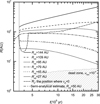 |
Fig. 1 Time evolution of the radial positions of clumps forming at different radii at t = 3.5 × 10⁵ yr in a protoplanetary disk with MMCC = 1 M⊙, TMCC = 15 K, and ω = 2.8 × 10⁻¹⁴ s−1. The adopted αmin is 10−4. Each line represents the time evolution of the radial position of a clump forming at a specific radius, Rinit. The solid, dashed, short-dashed, dash-dotted, dotted, and short-dotted lines represent the evolution of the radial positions for clumps forming at Rinit = 144 AU, 109 AU, 95 AU, 79 AU, 45 AU, and 27 AU, respectively. The dash-dot-dotted line represents the semi-analytical estimate from Appendix A for the evolution of the radial positions of a clump forming at 50 AU. The short-dash-dotted line represents the evolution of R0, the radial position where υR = 0. The shaded region shows the dead zone. The time t = 0 is set to be the beginning of the collapse of the parent cloud core. The vertical line indicates tinfall, the time when the collapse ends. We chose Rinit to be in the fragmentation region where the fragmentation conditions are satisfied. |
3 Numerical results of migration for clumps forming at different radii at different times
In this section, we consider clumps forming at different radii at different times in a disk. By using a time-evolution disk model and the type II migration rate, we follow the evolution of the radial positions of clumps throughout the whole disk lifetime.
3.1 Cases with fiducial dead zone viscosity
Figure 1 follows the migration of clumps after clump formation. Specifically, it shows the time evolution of the radial positions of clumps forming at different radii at t = 3.5 × 10⁵ yr (t = tinfall) in the prototype protoplanetary disk, namely, the disk with MMCC = 1 M⊙, TMCC = 15 K, and ω = 2.8 × 10⁻¹⁴ s−1. The adopted αmin is 10−4. We define Rinit to be the initial radial position of the migration, which is the radius where a clump forms. It can also be considered as the position after the initial phase of fast migration. We chose Rinit to be in the fragmentation region where the fragmentation conditions are satisfied because a clump can form only in the fragmentation region (if it can form). The largest Rinit is the outer boundary of the fragmentation region. The smallest Rinit is the inner boundary. We mention that the fragmentation region evolves with time (e.g., Tang & Jin 2019; Jin et al. 2020). Namely, the range of Rinit is different for clumps forming at different times. For Fig. 1, Rinit is in the fragmentation region at t = 3.5 × 10⁵ yr, the time when the mass influx onto the disk ends. Approximately, we use the disk median lifetime of 3.0 × 10⁶ yr (e.g., Haisch et al. 2001; Fedele et al. 2010; Richert et al. 2018) and the migration ends at t = 3.0 × 10⁶ yr. Please note that in Fig. 1, the migration process proceeds after the mass influx ends. In this case, the type II migration rate due to the mass influx drag in Eq. (23) is zero and clumps migrate by the migration rate only due to viscosity.
Ruden & Lin (1986) (see also Jin & Sui 2010) suggested that gas in the inner part of a disk moves inward and is accreted onto the protostar, while gas in the outer part expands outward. In the intermediate part, the gas flows outward first and then inward. Therefore, there is a radius, R0, at which υR = 0. In Fig. 1, the short-dash-dotted line represents the time evolution of R0. In general, R0 increases due to the disk expansion except that there is a pit between t = 3.5 × 10⁵ yr and 4.5 × 10⁵ yr. The sudden decrease in R0 at t = 3.5 × 10⁵ yr is due to the disappearance of the mass influx drag. As explained above (Eq. (23)), the influx contributes a negative value to υR. The disappearance of the influx leads to the increase in υR and the decrease in R0. The steep increase in R0 at t = 4.5 × 10⁵ yr is due to the transient process in which the disk adjusts from the configuration with the influx to the one without the influx.
In Fig. 1, the top two lines (the solid and dashed lines) with Rinit = 144 AU and 109 AU are outside R0 and the clumps migrate outward with disk expansion. The third line from the top (the short-dashed line) is outside R0 first and then inside R0 and the clump migrates outward first and then inward. The bottom three lines (the dash-dotted, dotted, and short-dotted lines) are inside R0 – except in the pit of R0 line and the clumps migrate inward except in the pit. The clump with Rinit = 144 AU (the outer boundary of the fragmentation region) migrates outward to 690 AU. The clump with Rinit = 27 AU (the inner boundary) migrates to 9 AU. The range of the final radial positions of clumps is 9-690 AU. In this case, even a clump forming at the inner boundary (the smallest initial radius) cannot fall on to the central protostar by the migration rate due to viscosity. We find that R0 plays an important role in clump migration. The final radius is sensitive to the initial radius. Even though the type II migration rate is low, clumps still migrate significant distances from their initial locations during the disk lifetime.
Figure 2 shows the same thing as Fig. 1, except that clumps form at a different time, t = 2.5 × 10⁵ yr (t < tinfall). The difference between Figs. 2 and 1 is that the clumps in Fig. 2 form before the collapse of the parent cloud core ends. Before the collapse ends, the mass influx drag contributes a negative value to υR at R < Rd(t) (Rd = 37 AU at t = 2.5 × 10⁵ yr and Rd = 102 AU at t = 3.5 × 10⁵ yr) and the influx maintains a surface density so that the gravitational instability viscosity is effective. Both effects enhance migration rate, υR. Therefore, in Fig. 2, the clumps migrate fast before t = 3.5 × 10⁵ yr. The first effect influences migration for Rinit ≤ 34 AU. Due to the enhancement of the migration rate, the clumps with Rinit ≤ 31 AU can migrate to the central protostar. We define Rinit,max as the maximum of initial radii from which clumps can migrate to the central star. The definition of Rinit,max means that clumps forming at a radius ≤ Rinit,max can migrate to the central star. Here, Rinit,max = 31 AU. The enhancement increases Rinit,max and more clumps migrate to the central protostar. On the contrary, in Fig. 1, we can see that no clumps migrate to the central protostar. We emphasize that in this paper, when we say “fall on to the central protostar” or “migrate to the central star,” we mean that a protoplanet migrates either to the central protostar or to a small radius, where it might be stopped by a stopping mechanism (Lin et al. 1996; Trilling et al. 1998; Miranda & Lai 2018; Romanova et al. 2019; Flock et al. 2019; Paardekooper et al. 2023, Sect. 3.8).
Figure 3 shows the migration of clumps forming at the inner and the outer boundary of the fragmentation region. Specifically, it shows time evolution of the radial positions of clumps forming at the inner and the outer boundary at different times in a protoplanetary disk with MMCC = 1 M⊙, TMCC = 15 K, and ω = 2.8 × 10⁻¹⁴ s−1. The adopted αmin is 10−4. The final radial position of any clump forming between the inner and the outer boundary is between those of the clumps forming at the inner and the outer boundary. Thus, we use the migration of the clumps forming at the inner and the outer boundary to describe characteristics of migration of clumps forming at a specific time. We note that the fragmentation region in Fig. 3 evolves with time. Before the mass influx from the parent cloud core ends, both the disk mass and Σ increase since there is a mass supply. Toomre parameter Q decreases. At t ~ 2 × 10⁵ yr, the disk gets enough mass to start to have fragmentation region. As the disk mass increase, the gravitationally unstable region expands and the fragmentation region expands. After the influx ends, Σ decreases as a result of the accretion onto the protostar and the mass spreading by viscosity and Q increases. Therefore, the unstable region and the fragmentation region shrink till they vanish (see Tang & Jin 2019 and Jin et al. 2020). At t ~ 8 × 10⁵ yr, the fragmentation region vanishes.
In Fig. 3, the slope change at t = 3.5 × 10⁵ yr is attributed to the halting of the mass influx. We find that clumps that form at relatively small radii before the influx ends can migrate to the central protostar or maybe to a stopping radius. No clumps that form after the influx ends migrate to the central protostar. We note that for clumps forming at a specific time, there is an Rinit,max and Rinit,max is different for different formation times. Considering all formation times, there is a maximum of Rinit,max for a disk. For the disk of Figs. 1, 2, and 3, the maximum of Rinit,max is 33 AU. The maximum of the final radii of clumps is ~800 AU.
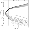 |
Fig. 2 Same as Fig. 1, except that clumps form at a different time, t = 2.5 × 10⁵ yr. The solid lines from the top to the bottom represent the evolution of the radial positions of clumps forming at Rinit = 55 AU, 52 AU, 50 AU, 48 AU, 45 AU, 43 AU, 41 AU, 40 AU, 38 AU, 36 AU, 34 AU, 33 AU, 31 AU, 30 AU, 29 AU, 27 AU, 26 AU, 25 AU, and 24 AU, respectively. The dash-dot-dotted line represents the semi-analytical estimate from Appendix A for the evolution of the radial positions of a clump forming at 37 AU. |
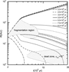 |
Fig. 3 Time evolution of the radial positions of clumps forming at the inner and the outer boundary of the fragmentation region at different times in a protoplanetary disk with MMCC = 1 M⊙, TMCC = 15 K, and ω = 2.8 × 10⁻¹⁴ s−1. The adopted αmin is 10−4. Using different line styles, we differentiate different clump-formation times. Each pair of the lines with the same style represents the time evolution of the radial positions of the clumps forming at the inner and the outer boundary at a specific time. The pairs of the dash-dotted, dashed, short-dashed, solid, short-dotted, dotted, and short-dash-dotted lines represent the evolution of the radial positions of clumps forming at 2.0 × 10⁵ yr, 2.5 × 10⁵ yr, 3.0 × 10⁵ yr, 3.5 × 10⁵ yr, 5.5 × 10⁵ yr, 7.5 × 10⁵ yr, and 8.2 × 10⁵ yr, respectively. The fragmentation region and the dead zone are shown as shaded regions. Other information is the same as Fig. 1. |
3.2 Cases with high dead zone viscosity
Figure 4 shows the same details as Fig. 1, except that αmin = 10−3 and clumps form at 5.6 × 10⁵ yr. In both Figs. 4 and 1, the migration process proceeds after the mass influx ends and clumps migrate by the migration rate due to viscosity. The difference between Figs. 4 and 1 is that the viscosity αmin and therefore, migration rate in the dead zone in Fig. 4 are higher than those in Fig. 1. Due to the higher migration rate in Fig. 4, clumps with Rinit < 29 AU can migrate to the central protostar. On the contrary, no clumps in Fig. 1 migrate to the central protostar.
Figure 5 shows the same thing as Fig. 2, except that αmin = 10−3 and clumps form at 2.8 × 10⁵ yr. In both Figs. 5 and 2, clumps form before the mass influx ends and they migrate by both the mass influx drag and viscosity. The difference between Figs. 5 and 2 is that the viscosity αmin and, therefore, the migration rate in the dead zone in Fig. 5 are higher than those in Fig. 2. Due to the higher migration rate in the dead zone in Fig. 5, clumps with Rinit < 41 AU can migrate to the central protostar, Rinit,max (= 41 AU) is increased and more clumps migrate to the central protostar, compared to Fig. 2.
Figure 6 shows the same thing as Fig. 3, except for αmin = 10−3. The difference between Figs. 6 and 3 is that the viscosity αmin and migration rate in the dead zone in Fig. 6 are higher than those in Fig. 3. Due to the higher migration rate in the dead zone in Fig. 6, some clumps forming at relatively small radii after the mass influx ends can migrate to the central protostar by viscosity migration. On the contrary, in Fig. 3, no clumps that form after the influx ends migrate to the central protostar. For the disk of Figs. 4, 5, and 6, the maximum of Rinit,max is 41 AU. As αmin is increased to 10−3, Rinit,max is increased and more clumps migrate to the central protostar, compared to Figs. 1, 2, and 3.
Comparing the results of αmin = 10−3 to those of αmin = 10−4, the viscosity (of order of magnitude) in the dead zone makes the difference and its uncertainty lead to further uncertainties in the calculations of migration. We also show the results of the semi-analytical estimate from Appendix A for the evolution of the radial positions of clumps in Figs. 1, 2, 4, and 5. We find that the semi-analytical estimates in Appendix A are consistent with numerical calculations. In the next section, we study the dependence of clump migration on the properties of the parent cloud core.
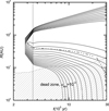 |
Fig. 5 Same as Fig. 2, except that αmin = 10−3 and clumps form at 2.8 × 10⁵ yr. The dash-dot-dotted line represents the semi-analytical estimate from Appendix A for the evolution of the radial positions of a clump forming at 3.0 × 10⁵ yr at 57 AU. |
4 Dependence of clump migration on the properties of the parent cloud core
As stated in Sect. 1, the mass influx used in our disk model reflects the effects of the parent cloud core properties on the disk and, therefore, on giant planet formation by disk instability. With the disk model, we investigate the dependence of the clump migration on the properties. In this section, we present the numerical results of migration calculations with a wide range of parameters of cloud core properties.
4.1 Dependence on angular velocity of cloud core
In Fig. 7, we show the dependence of clump migration on ω in disks with MMCC = 1 M⊙ and TMCC = 15 K. Specifically, Fig. 7 shows the time evolution of the radial positions of the clumps forming at the inner and the outer boundary of the fragmentation region at t = 3.5 × 10⁵ yr (the time when the collapse of the parent cloud core ends, namely, t = tinfall) in different disks with different ω. Considering the time evolution of the fragmentation region, for comparison, for each disk, we chose the clumps forming at t = tinfall. This time is not a function of ω (e.g., Jin & Li 2014). We chose this time as the representative. At this time during the disk evolution, the disk mass reaches the maximum and the outer boundary reaches its maximum radius.
In Fig. 7, clumps forming at the outer boundary are outside R0 and migrate outward. As ω increases, the angular momentum increases, the more mass continues to spread across a large radius, and the mass of the disk increases. Therefore, both R0 and the outer boundary increases with ω. For high ω (5.0 × 10⁻¹⁴ s−1 and 8.0 × 10⁻¹⁴ s−1), the clumps forming at the inner boundary are always inside R0. They always migrate inward. Therefore, clumps forming at relatively small radii migrate to the central protostar and more clumps migrate to the central protostar. On the contrary, for relatively low ω (1.5 × 10⁻¹⁴ s−1, 2.0 × 10⁻¹⁴ s−1, and 2.8 × 10⁻¹⁴ s−1), the clumps forming at the inner boundary are outside R0 first and then inside R0 and they migrate outward first and then inward. Therefore, they do not migrate to the central protostar. We mention that for small ω (approximately ω < 1.1 × 10⁻¹⁴ s−1), there is not enough matter spreading to the disk and the disk is stable.
As ω increases, both R0 and Rd (see Eq. (3)) increase, and also fragmentation duration increases (Jin et al. 2020). As discussed above, the increase in R0 enhances the inward migration. The increase in Rd expands the area where the mass influx drag can enhance the inward migration. The increase in the fragmentation duration is equivalent to the increase in the duration of gravitational instability and the effect of gravitational instability viscosity lasts longer. Also, Jin et al. (2020) suggested that as ω increases, gravitational instability becomes effective early, fragmentation starts early and clumps can form early. Clumps forming early experience the mass influx drag and gravitational instability for a longer time and migrate longer distance. This effect is shown in Fig. 8. As ω increases, all the above effects enhance the migration rate and increase Rinit,max. Also, the increase in the fragmentation duration increases the probability that clumps can form. Therefore, more clumps migrate to the central star. For clumps forming at 3.5 × 10⁵ yr (t = tinfall), clumps forming at the inner boundary of the fragmentation region do not migrate to the central star for ω = 1.5 × 10⁻¹⁴ s−1, 2.0 × 10⁻¹⁴ s−1, and 2.8 × 10⁻¹⁴ s−1 and Rinit,max = 28 AU and 44 AU for ω = 5.0 × 10⁻¹⁴ s−1 and 8.0 × 10⁻¹⁴ s−1, respectively. For clumps forming at 2.5 × 10⁵ yr (<tinfall), clumps forming at the inner boundary do not migrate to the central star for ω = 1.5 × 10⁻¹⁴ s−1 and 2.0 × 10⁻¹⁴ s−1 and Rinit,max= 31 AU, 69 AU, and 95 AU for ω = 2.8 × 10⁻¹⁴ s−1, 5.0 × 10⁻¹⁴ s−1, and 8.0 × 10⁻¹⁴ s−1, respectively. The maximum of Rinit,max is 33 AU, 71 AU, and 111 AU for ω = 2.8 × 10⁻¹⁴ s−1, 5.0× 10⁻¹⁴ s−1, and 8.0 × 10⁻¹⁴ s−1, respectively.
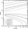 |
Fig. 7 Dependence of clump migration on ω in disks with MMCC = 1 M⊙ and TMCC = 15 K. Using different line styles, we differentiate different ω values. Each pair of the lines with the same style represents the time evolution of the radial positions of the clumps forming at the inner and the outer boundary of the fragmentation region at t = 3.5 × 10⁵ yr (time when the collapse of the parent cloud core ends) in a protoplanetary disk with a specific ω. The pairs of the dotted, short-dotted, solid, short-dashed, and dashed lines represent the evolution of the radial positions of clumps forming in disks with ω = 1.5 × 10⁻¹⁴ s−1, 2.0 × 10⁻¹⁴ s−1 2.8 × 10⁻¹⁴ s−1 5.0 × 10⁻¹⁴ s−1 and 8.0 × 10⁻¹⁴ s−1 respectively. The other information is the same as Fig. 1. |
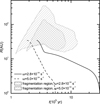 |
Fig. 8 Effect of the early formation of the clump with different ω. This figure shows the time evolution of the radial positions of clumps forming at the same radius Rinit = 34 AU in different disks with different ω and the same MMCC = 1 M⊙ and TMCC = 15 K. The solid line represents the evolution of the radial position of a clump forming at i = 2.7 × 10⁵ yr in a disk with ω = 2.8 × 10⁻¹⁴ s−1 and the dashed line represents that of a clump forming at i = 1.8 × 10⁵ yr in a disk with ω = 5.0 × 10⁻¹⁴ s−1. The shaded regions indicate the fragmentation regions, which refer to when and where the fragmentation conditions are satisfied. |
4.2 Dependence on cloud core temperature
In Fig. 9, we show the dependence of clump migration on TMCC in disks with MMCC = 1 M⊙ and ω = 2.8 × 10⁻¹⁴ s−1. Specifically, Fig. 9 shows the time evolution of the radial positions of the clumps forming at the inner and the outer boundary of the fragmentation region at t = tinfall in different disks with different TMCC. We note that from Eq. (5), tinfall decreases with TMCC. Considering the time evolution of the fragmentation region, for comparison, we chose the clumps forming at t = tinfall for each disk. As in Fig. 7, we chose this as the representative time.
In Fig. 9, clumps forming at the outer boundary are outside R0 and migrate outward. From Eq. (4), the angular momentum of a molecular cloud core increases with decreasing TMCC. Thus, the effects on the migration caused by the decrease in TMCC are similar to those caused by the increase in ω. As TMCC decreases, namely, the angular momentum increases, more mass spreads to large radius and the mass of a disk increases. Therefore, both R0 and the outer boundary increase with decreasing TMCC. For low TMCC (10 K and 12 K), the clumps forming at the inner boundary are inside R0. They always migrate inward. Therefore, they migrate to small radii. On the contrary, for relatively high TMCC (15 K, 18 K, and 20 K), the clumps forming at the inner boundary are outside R0 first and then inside R0 and they migrate outward first and then inward. Therefore, they do not migrate to small radii. We mention that for high TMCC (approximately TMCC > 24 K), there is not enough matter spreading to the disk and the disk is stable.
As TMCC decreases, both R0 and tinfall (see Eq. (5)) increase, and also fragmentation duration increases (Jin et al. 2020). As tinfall increases, Rd increases (see Eqs. (5) and (3)). As TMCC decreases, as discussed above, all the above effects enhance the migration rate and increase Rinit,max. Also, as TMCC decreases, tinfall increases and the mass influx drag are effective for a longer time. Clumps forming at t < tinfall experience the mass influx drag for a longer time. This also enhances the migration rate and increases Rinit,max. Also, the increase in the fragmentation duration increases the probability that clumps can form. Therefore, more clumps migrate to the central star. For clumps forming at t = tinfall, clumps forming at the inner boundary of the fragmentation region do not migrate to the central star for TMCC = 12 K, 15 K, 18 K, and 20 K and Rinit,max = 24 AU for TMCC = 10 K. For clumps forming at t = 0.8 tinfall, clumps forming at the inner boundary do not migrate to the central star for TMCC = 18 K and 20 K and Rinit,max = 57 AU, 48 AU, and 33 AU for TMCC = 10 K, 12 K, and 15 K, respectively. The maximum of Rinit,max is 87 AU, 58 AU, and 33 AU for TMCC = 10 K, 12 K, and 15 K, respectively.
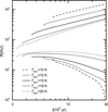 |
Fig. 9 Dependence of clump migration on TMCC in disks with MMCC = 1 M⊙ and ω = 2.8 × 10⁻¹⁴ s−1. Using different line styles, we differentiate different TMCC. Each pair of the lines with the same style represents the time evolution of the radial positions of the clumps forming at the inner and the outer boundary of the fragmentation region at t = tinfall in a protoplanetary disk with a specific TMCC. The pairs of the dashed, short-dashed, solid, short-dotted, and dotted lines represent the evolution of the radial positions of clumps forming in disks with TMCC = 10 K, 12 K, 15 K, 18 K, and 20 K, respectively. Other information is the same as Fig. 1. |
4.3 The dependence on cloud core mass
In Fig. 10, we show the dependence of clump migration on MMCC in disks with TMCC = 15 K and ω = 2.8 × 10⁻¹⁴ s−1. Specifically, Fig. 10 shows the time evolution of the radial positions of the clumps forming at the inner and the outer boundary of the fragmentation region at t = tinfall in different disks with different MMCC. We note that based on Eq. (5), we see that tinfall increases with MMCC. Considering the time evolution of the fragmentation region, for comparison, for each disk, we chose the clumps forming at t = tinfall.
In Fig. 10, clumps forming at the outer boundary are outside R0 and migrate outward. The increase in MMCC adds more matter with high specific angular momentum to the disk, more matter spreads outward in the disk, and the disk mass increases. Both R0 and the outer boundary increases with MMCC. For high MMCC (1.2 M⊙ and 1.5 M⊙), the clumps forming at the inner boundary are inside R0. They always migrate inward. Therefore, they migrate to small radii. On the contrary, for relatively low MMCC (0.6 M⊙, 0.8 M⊙, and 1.0 M⊙), the clumps forming at the inner boundary are outside R0 first and then inside R0; then, they migrate outward first and then inward. Therefore, they do not migrate to small radii. We mention that for small MMCC (approximately MMCC < 0.6 M⊙), there is not enough matter spreading to the disk and the disk is stable.
As MMCC increases, both R0 and tinfall (see Eq. (5)) increase, and also fragmentation duration increases (Jin et al. 2020). As discussed above, all these effects lead to the increase in the migration rate and Rinit,max. Also, for higher MMCC, the gravitational instability is stronger and its viscosity is higher. This effect enhances the migration rate as MMCC increases. Further, the increase in the fragmentation duration increases the probability that clumps can form. Therefore, more clumps migrate to the central star. For clumps forming at t = tinfall in Fig. 10, the final radius of the clumps forming at the inner boundary of the fragmentation region decreases with MMCC. For clumps forming at t = 0.8 tinfall, clumps forming at the inner boundary do not migrate to the central star for MMCC = 0.6 M⊙ and 0.8 M⊙ and Rinit,max = 33 AU, 43 AU, and 57 AU for MMCC = 1.0 M⊙, 1.2 M⊙, and 1.5 M⊙, respectively. The maximum of Rinit, max is 33 AU, 48 AU, and 71 AU for Mmcc = 1.0 M⊙, 1.2 M⊙, and 1.5 M⊙, respectively. From our calculations in Sect. 3 and this section, we find that a considerable proportion of clumps migrate to the central protostar by type II migration.
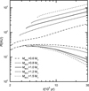 |
Fig. 10 Dependence of clump migration on MMCC in disks with TMCC = 15 K and ω = 2.8 × 10⁻¹⁴ s−1. Using different line styles, we differentiate different MMCC. Each pair of the lines with the same style represents the time evolution of the radial positions of the clumps forming at the inner and the outer boundary of the fragmentation region at t = tinfall in a protoplanetary disk with a specific MMCC. The pairs of the dashed, short-dashed, solid, short-dotted, and dotted lines represent the evolution of the radial positions of clumps forming in disks with MMCC = 0.6 M⊙, 0.8 M⊙, 1.0 M⊙, 1.2 M⊙, and 1.5 M⊙, respectively. Other information is the same as Fig. 1. |
5 Discussion
There are numerous phenomena that are not considered that may affect migration in this paper. We do not consider the initial phase of fast migration, which is typically on a short timescale. If this happens, our initial position can be considered as the position after the initial phase. During the initial phase, clumps migrate several tens of AU. The overall effect of the initial phase is to enhance the migration and make more clumps to migrate to the central protostar. We do not consider effects near the inner disk edge, such as the stellar magnetic field, on migration (for a review on this specific topic, see Sect. 3.8 of Paardekooper et al. 2023; see also Lin et al. 1996 and Trilling et al. 1998). For cases where clumps can migrate to the inner disk edge in our calculations, those effects near the edge may play a role in the clump migration and the results from the studies of those effects can be applicable. The effects near the inner disk edge might lead to the stop of a clump at a small radius (e.g., Lin et al. 1996; Trilling et al. 1998; Paardekooper et al. 2023, Sect. 3.8). Michael et al. (2011) suggested that interaction with spiral modes might affect migration. The time length of their simulations is a few thousand years. Their results of planet migration are shown in their Fig. 2. From their Fig. 2, a planet appears to fluctuate with fluctuations of several AU. But the overall trend is that there is an initial fast migration and then a planet slows down. We do not think that this interaction can affect the subsequent long term slow migration. Vorobyov & Elbakyan (2018) investigated the migration of clumps. They have just one simulation run. In their run, all clumps form at > 100 AU. Four clumps can be seen in their Fig. 3. Three of them have no significant migration. One of them migrates fast initially and then the tidal mass loss substantially slows down or maybe even stops the clump inward migration at a few tens of AU. At the end of their run, all clumps are tidally destroyed. They think that this is due to the neglect of the possible clump contraction to planetary sized objects. To summarize, we do not think that the effects discussed in this paragraph can affect the general trend of the calculations of type II migration during the disk lifetime.
As discussed above, at this point, due to many uncertainties in the planet formation theory, it is difficult to compare theoretical calculations to observations exactly. Although the final orbital radii of planets are affected by many physical factors, we attempt to use the results of our calculations to understand observations. One of the outstanding observations is that a large number of planets pile up at semi-major axes less than 0.3 AU. A possible explanation is that a planet might form at a large radius, then migrate to an orbit of <0.3 AU and halt there by a stopping mechanism (Lin et al. 1996; Trilling et al. 1998; Miranda & Lai 2018; Romanova et al. 2019; Flock et al. 2019; Paardekooper et al. 2023, Sect. 3.8). One of the results of our calculations is that a considerable proportion of clumps migrate to the central protostar by type II migration. If there is an initial phase of fast migration, in which a clump can migrate to a smaller radius from its formation location (see references in Sect. 1), more clumps can migrate to the central protostar. Therefore, our calculations support the above explanation. As we note, when we mention “fall on to the central protostar” or “migrate to the central star,” we mean that a protoplanet migrates either to the central protostar or to a small radius where it might be stopped by a stopping mechanism.
We think that the length of disk lifetime is critical to explain the observed pile-up of planets at <0.3 AU. Even though the type II migration rate is low, a considerable proportion of clumps migrate to the central protostar due to the long disk lifetime. If the lifetime is short, clumps cannot migrate significant distance. The disk lifetime is obtained from observations and is reliable. Among the enhancement mechanisms of migration discussed in Sects. 3 and 4, we think that the mass influx drag is relatively more important to explain the observation of many close-in giant planets since the acceleration due to the mass influx drag is more significant. The disk model and the disk instability model come from physics. The enhancement mechanisms come from the disk model and disk instability model. From this point of view, we think that they are all likely to occur.
6 Conclusions
Using a numerical time-evolution disk model and the type II migration rate, we follow the evolution of the radial positions of clumps formed by gravitational instability throughout the disk lifetime to study the effects of type II migration on the final orbital positions of gas giant planets. We consider clumps forming at different radii at different times and study the dependence of the clump migration on the properties of the parent core. Our conclusions are the following:
- 1.
Even though the type II migration rate is low, clumps still migrate significant distances from their initial positions during the disk lifetime. These initial positions can be either the formation locations of clumps or the positions after the initial phase of fast migration;
- 2.
The final radius is sensitive to the initial radius. Clumps forming at relatively small radii can migrate to the central protostar;
- 3.
Clumps outside R0, the radius at which the radial velocity of gas υR = 0, migrate outward with disk expansion and clumps inside R0 migrate inward;
- 4.
The mass influx drag and the increases in the dead zone viscosity, the duration of gravitational instability, and the collapse time of the parent core enhance migration;
- 5.
Clumps forming before the mass influx ends tend to migrate across longer distance and are more likely to migrate to the central star;
- 6.
As ω increases, TMCC decreases and MMCC increases, thereby enhancing migration;
- 7.
A considerable proportion of clumps migrate to the central protostar by type II migration;
- 8.
The results of our calculations support the idea that the observed pile up of planets at <0.3 AU is explained by the scenario that planets might form at large radii, then migrate to orbits of <0.3 AU, and are halted there by a stopping mechanism.
Acknowledgements
We thank the referee for very helpful comments to improve the manuscript. This research has been supported in part by the National Natural Science Foundation of China (NSFC) grant 11373019.
Appendix A Semi-analytical estimates of migration
In this appendix, we describe how we carried out semi-analytical estimates for the migration of clumps. The results of our semi-analytical estimates confirm our numerical calculations. In the estimates, we use α values from our numerical calculations of the evolutionary disk model. We also used the analytical disk model suggested by Tang & Jin (2019), in which a disk is divided into three regions where the heating is dominated by the internal dissipation, the central protostar irradiation, and background irradiation, respectively, when the disk can extend to large radius (> 120 AU, see Tang & Jin 2019 and Jin et al. 2020). The evolution of self gravitating disks has been extensively explored (e.g., Rice et al. 2003; Lodato & Rice 2004; Mejía et al. 2005; Durisen et al. 2007), and it is believed that these disks reach a state with constant Q near Qcr.
We first consider the case where the mass influx onto the disk from the collapse of the parent molecular cloud core has ended. In this case, the type II migration rate due to the mass influx drag in Eq. (23) is zero and we need to consider only the migration rate due to viscosity. We first consider the migration in the protostar irradiation region (roughly, 20-140 AU). In this region, Σ can be expressed as (Tang & Jin 2019):
 (A.1)
(A.1)
and H/R can be expressed as
 (A.2)
(A.2)
Using Eq. (6) and cs = HΩ (Pringle 1981), we get
 (A.3)
(A.3)
Inserting Eq. (A.3) into Eq. (24), we obtain type II migration rate due to viscosity,
![${\upsilon _R} = - 3\alpha {\left( {{H \over R}} \right)^2}R{\rm{\Omega }}\left[ {{{\partial \ln \alpha } \over {\partial \ln R}} + 2 \times {{\partial \ln (H/R)} \over {\partial \ln R}} + {{\partial \ln {\rm{\Sigma }}} \over {\partial \ln R}} + 1} \right].$](/articles/aa/full_html/2024/05/aa48347-23/aa48347-23-eq31.png) (A.4)
(A.4)
For our rough estimates of migration in this section, we used α values from our numerical calculations of the evolutionary disk and consider the disk with the typical cloud core parameters: MMCC = 1 M⊙, TMCC = 15 K, and ω = 2.8 × 10⁻¹⁴ s−1. For this disk, the mass influx ends at t = tinfall = 3.5 × 10⁵ yr. We use α at t = 106 yr. Numerically calculated α values are shown in Fig. A.1. The solid line represents α in a disk with αmin = 10−4. In the dead zone (~1.3 – 5 AU) of the protoplanetary disk, α = αmin = 10−4. The innermost region (≤ 1 .3 AU) is partially ionized forthe MRI to partly operate since the disk temperature is relatively high. At ~5 – 80 AU, the main contribution to α is αGI. In the outermost region near the edge (> 100 AU) where the surface density is low, the MRI is active due to cosmic ray ionization (Jin 1996; Gammie 1996) and α ~ 0.8 × 10⁻² (Fleming & Stone 2003). The dashed line represents α in a disk with αmin = 10−3 and the situation is similar to the case of αmin = 10−4. From Fig. A.1, at 20 – 80 AU, α can be approximated as α ≈ 6.7 × 10⁻⁴(R/AU)0.43. Inserting this α and Eqs. (A.1) and (A.2) into Eq. (A.4) and taking M* = 1 M⊙, we get an approximate formula for υR,
 (A.5)
(A.5)
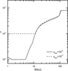 |
Fig. A.1 Numerically calculated α as a function of R at t = 106 yr in protoplanetary disks with the parent cloud core properties: MMCC = 1 M⊙, TMCC = 15 K, and ω = 2.8 × 10⁻¹⁴ s−1. The solid and dashed lines represent α in disks with αmin = 10−4 and 10−3, respectively. |
Since υR = dR/dt and dt = dR/υR, for a clump to migrate from R1 to R2, it takes time:
![$\matrix{ {{t_{{\rm{mig}},1}} = \mathop \smallint \nolimits^ _{{R_1}}^{{R_2}}{1 \over {{v_R}}}{\rm{d}}R = - \mathop \smallint \nolimits^ _{{R_1}}^{{R_2}}5.3 \times {{10}^5}{{\left( {{R \over {{\rm{AU}}}}} \right)}^{ - 0.50}}{\rm{d}}R} \cr { = 1.1 \times {{10}^6}\left[ {{{\left( {{{{R_1}} \over {{\rm{AU}}}}} \right)}^{0.50}} - {{\left( {{{{R_2}} \over {{\rm{AU}}}}} \right)}^{0.50}}} \right]{\rm{yr}}.} \cr } $](/articles/aa/full_html/2024/05/aa48347-23/aa48347-23-eq33.png) (A.6)
(A.6)
If we take R1 = 50 AU and R2 = 20 AU, the migration time is 2.7 × 10⁶ yr. Roughly, a clump forming at > 50 AU cannot migrate to 20 AU (the boundary between the internal dissipation region and the protostar irradiation region) and therefore does not fall on to the central protostar in the disk lifetime (~3 Myr, e.g., Haisch et al. 2001, Fedele et al. 2010, and Richert et al. 2018) with type II migration and a clump forming at <50 AU might migrate to <20 AU.
For the estimation of migration in the internal dissipation region (at <20 AU), we assume the steady state disk. Inserting Eq. (A.3) into Eq. (25), the migration rate becomes
 (A.7)
(A.7)
The migration rate depends on α and H/R. For a rough estimate, we take H/R = 0.08 and consider two cases: αmin = 10−4 or 10−3. For αmin = 10−4, at 1 – 5 AU, α = αmin = 10−4 and υR = −6.0 × 10⁻⁶(R/AU)−1/2 AU yr−1. For a clump to migrate from 5 AU to 1 AU, it takes time
 (A.8)
(A.8)
In this case, a clump takes a million years to migrate through the dead zone. From Fig. A.1, at 5 – 20 AU, α can be approximated as α ≈ 3.0 × 10⁻⁶(R/AU)2.3. Inserting this α into Eq. (A.7) and taking M* = 1 M⊙, we get υR = −1.8 × 10⁻⁷(R/AU)1.8 AU yr−1. For a clump to migrate from 20 AU to 5 AU, it takes time, as per:
 (A.9)
(A.9)
Thus, tmig,2 + tmig,3 ≈ 2.4 × 10⁶ yr ≈disk lifetime. Roughly, a clump at <20 AU (near the inner boundary of the fragmentation region) can fall on to the central protostar in the disk lifetime. Here, Rinit,max = 20 AU.
For the case of αmin = 10−3, at 1 − 11 AU, α = αmin = 10−3. From Eq. (A.7), taking M* = 1 M⊙, υR = −6.0 × 10⁻⁵(R/AU)−1/2 AU yr−1. For a clump to migrate from 11 AU to 1 AU, it takes time
 (A.10)
In this case, a clump takes 3.9 × 10⁵ yr to migrate through the dead zone. From Fig. A.1, at 11 − 20 AU, α can be approximated as α ≈ 2.8 × 10⁻⁵(R/AU)1.5. Inserting this α into Eq. (A.7) and taking M* = 1 M⊙, we get υR = −1.7 × 10⁻⁶(R/AU)1.0 AU yr−1. For a clump to migrate from 20 AU to 11 AU, it takes time, as per:
 (A.11)
From Eq. (A.6), it takes tmig,1 = 2.0 × 10⁶ yr for a clump to migrate from 40 AU to 20 AU. Thus, tmig,4 + tmig,4 + tmig,5 ≈ 2.7 × 10⁶ yr ≈ disk lifetime. Roughly, a clump forming at <40 AU can fall on to the central protostar in the disk lifetime; namely, Rinit, max = 40 AU. The viscosity αmin and migration rate in the dead zone in the case of αmin = 10−3 are higher than those in the case of αmin = 10−4. Due to the higher migration rate in the case of αmin = 10−3, Rinit,max is increased.
We now consider the effects of the migration rate due to the mass influx drag in Eq. (23) and the rate can be written as:
![${\upsilon _{R,{\rm{influx}}}} = - {{2RS} \over {\rm{\Sigma }}}\left[ {1 - {{\left( {{R \over {{R_{\rm{d}}}}}} \right)}^{1/2}}} \right]{\rm{.}}$](/articles/aa/full_html/2024/05/aa48347-23/aa48347-23-eq39.png) (A.12)
(A.12)
This rate is non-zero at R < Rd and only before the mass influx onto the disk ends (at t < tinfall = 3.5 × 10⁵ yr). Inserting Eqs. (2) and (3) into (A.12), we get
 (A.13)
In the above calculations for αmin = 10−4, a clump at <20 AU can fall on to the protostar with the viscous migration rate in the disk lifetime. Thus, we only need to consider whether the migration rate due to the mass influx drag can migrate a clump to 20 AU before the mass influx ends. Roughly, R > 20 AU is in the protostar irradiation region. Inserting Σ in this region (Eq. (A.1)) into Eq. (A.13), we have
 (A.14)

and we have used Q = 1 and M* = 0.5 M⊙ in Eq. (A.1). We take M* = 0.5 M⊙ because not all of the mass of the parent core has fallen onto the protostar+disk system and been accreted onto the protostar when υR,influx is non-zero. The factor, f, increases with time since R decreases and Rd increases with time. Therefore, f reaches its maximum at 3.5 × 10⁵ yr (t = tinfall) and Rd expands to ~ 100 AU. If we assume that a clump migrates to R = 20 AU at the end of the mass influx, the maximum value of f is 0.6. We consider υR,influx at a typical radius, R = 30 AU. If Rd = 30 AU, f = 0. When Rd > 30 AU, f increases as Rd expands. At t = 2.4 × 10⁵ yr, Rd = 34 AU, f = 0.1. We take this time as when υR,influx starts to be effective at R = 30 AU. So on average, we take t = 3 × 10⁵ yr and f = 0.4 in Eq. (A.14) and get υR,influx = −1.9 × 10⁻⁴ AU yr−1, which is an order of magnitude higher than Eq. (A.5). Using υR = dR/dt and dt = dR/υR, from Eq. (A.14), we get
 (A.16)
We consider that a clump migrates from R1 to R2 during the time from t1 to t2. After rearranging the above equation and integrating, we obtain
 (A.17)
![$\matrix{ {{{\left( {{{{t_1}} \over {3.5 \times {{10}^5}{\rm{yr}}}}} \right)}^{ - 2}} - {{\left( {{{{t_2}} \over {3.5 \times {{10}^5}{\rm{yr}}}}} \right)}^{ - 2}}} \hfill \cr { = 23{{\left( {{{{T_{{\rm{MCC}}}}} \over {15{\rm{K}}}}} \right)}^{ - 1}}{{\left( {{\omega \over {2.8 \times {{10}^{ - 14}}{{\rm{s}}^{ - 1}}}}} \right)}^2}\left[ {{{\left( {{{{R_2}} \over {{\rm{AU}}}}} \right)}^{ - 5/7}} - {{\left( {{{{R_1}} \over {{\rm{AU}}}}} \right)}^{ - 5/7}}} \right].} \hfill \cr } $](/articles/aa/full_html/2024/05/aa48347-23/aa48347-23-eq45.png)
We are interested in determining the radius from which a clump can migrate to 20 AU at 3.5 × 10⁵ yr. From Eq. (A.18), we find that if a clump forms at 37 AU at t1 = 2.5 × 10⁵ yr (Rd expands to 38 AU at this time), it can migrate to 20 AU. We conclude that for αmin = 10−4, with the help of the mass influx drag, a clump forming at <40 AU can migrate to the central star. The mass influx drag enhances the migration rate and increases Rinit,max.
For the case of αmin = 10−3, we find above that the migration rate due to viscosity can make a clump forming at <40 AU fall on to the central protostar in the disk lifetime. We are interested in determining the radius from which a clump can migrate to 40 AU at 3.5 × 10⁵ yr due to the mass influx drag. From Eq. (A.18), we find that if a clump forms at 57 AU at t1 = 3.0 × 10⁵ yr (Rd expands to 66 AU at this time), it can migrate to 40 AU. We conclude that with the help of the mass influx drag, a clump forming at <60 AU can migrate to the central star.
The results of this section can be summarized as the following. In the case of αmin = 10−4, a clump forming at <20 AU (near the inner boundary of the fragmentation region) can fall on to the central protostar in the disk lifetime by the migration rate due to viscosity. With the help of the mass influx drag, a clump forming at <40 AU can migrate to the central star. In the case of αmin = 10−3, a clump forming at <40 AU can fall on to the central protostar in the disk lifetime by the migration rate due to viscosity. With the help of the mass influx drag, a clump forming at <60 AU can migrate to the central star. We can see that the magnitude of the viscosity in the dead zone causes the difference of the migration results and the mass influx drag enhances the migration rate and increases Rinit,max. Also, a clump forming at <50 AU can migrate to <20 AU in the disk lifetime by the migration rate due to viscosity without the help of the mass influx drag. We mention that the results of the estimates in this section depend on the choices of the parameters.
References
- Armitage, P. J. 2010, Astrophysics of Planet Formation (Cambridge University Press) [Google Scholar]
- Armitage, P. J. 2011, ARA&A, 49, 195 [Google Scholar]
- Armitage, P. J. 2019, Physical Processes in Protoplanetary Disks (Springer Berlin Heidelberg), 1 [Google Scholar]
- Baruteau, C., Crida, A., Paardekooper, S.-J., et al. 2014, Protostars and Planets VI, 667 [Google Scholar]
- Boss, A. P. 2000, ApJ, 536, L101 [CrossRef] [Google Scholar]
- Caselli, P., Benson, P. J., Myers, P. C., & Tafalla, M. 2002, ApJ, 572, 238 [Google Scholar]
- Cassen, P., & Moosman, A. 1981, Icarus, 48, 353 [CrossRef] [Google Scholar]
- Chabrier, G., Johansen, A., Janson, M., & Rafikov, R. 2014, Protostars and Planets VI, 619 [Google Scholar]
- Chiang, E. I., & Goldreich, P. 1997, ApJ, 490, 368 [Google Scholar]
- Clarke, C. J. 2009, MNRAS, 396, 1066 [Google Scholar]
- D’Angelo, G., Durisen, R. H., & Lissauer, J. J. 2011, Exoplanets, 319 [Google Scholar]
- Drążkowska, J., Bitsch, B., Lambrechts, M., et al. 2023, ASP Conf. Ser., 534, 717 [NASA ADS] [Google Scholar]
- Durisen, R. H., Boss, A. P., Mayer, L., et al. 2007, Protostars and Planets V, 607 [Google Scholar]
- Dürmann, C., & Kley, W. 2015, A&A, 574, A52 [NASA ADS] [CrossRef] [EDP Sciences] [Google Scholar]
- Fedele, D., Van Den Ancker, M. E., Henning, T., Jayawardhana, R., & Oliveira, J. M. 2010, A&A, 510, A72 [NASA ADS] [CrossRef] [EDP Sciences] [Google Scholar]
- Fleming, T., & Stone, J. M. 2003, ApJ, 585, 908 [NASA ADS] [CrossRef] [Google Scholar]
- Fletcher, M., Nayakshin, S., Stamatellos, D., et al. 2019, MNRAS, 486, 4398 [NASA ADS] [CrossRef] [Google Scholar]
- Flock, M., Turner, N. J., Mulders, G. D., et al. 2019, A&A, 630, A147 [NASA ADS] [CrossRef] [EDP Sciences] [Google Scholar]
- Frank, J., King, A., & Raine, D. 2002, Accretion Power in Astrophysics (Cambridge University Press) [Google Scholar]
- Gammie, C. F. 1996, ApJ, 457, 355 [Google Scholar]
- Gammie, C. F. 2001, ApJ, 553, 174 [Google Scholar]
- Goldreich, P., & Tremaine, S. 1980, ApJ, 241, 425 [Google Scholar]
- Goodman, A. A., Benson, P. J., Fuller, G. A., & Myers, P. C. 1993, ApJ, 406, 528 [Google Scholar]
- Haisch, K. E. Jr., Lada, E. A., & Lada, C. J. 2001, ApJ, 553, L153 [NASA ADS] [CrossRef] [Google Scholar]
- Hartmann, L., & Bae, J. 2018, MNRAS, 474, 88 [NASA ADS] [CrossRef] [Google Scholar]
- Helled, R., Bodenheimer, P., Podolak, M., et al. 2014, Protostars and Planets VI, 643 [Google Scholar]
- Hueso, R., & Guillot, T. 2005, A&A, 442, 703 [NASA ADS] [CrossRef] [EDP Sciences] [Google Scholar]
- Jijina, J., Myers, P. C., & Adams, F. C. 1999, ApJS, 125, 161 [Google Scholar]
- Jin, L. 1996, ApJ, 457, 798 [NASA ADS] [CrossRef] [Google Scholar]
- Jin, L. 2010, ApJ, 720, L211 [Google Scholar]
- Jin, L., & Li, M. 2014, ApJ, 783, 37 [NASA ADS] [CrossRef] [Google Scholar]
- Jin, L., & Sui, N. 2010, ApJ, 710, 1179 [NASA ADS] [CrossRef] [Google Scholar]
- Jin, L., Liu, F., Jiang, T., Tang, P., & Yang, J. 2020, ApJ, 904, 55 [NASA ADS] [CrossRef] [Google Scholar]
- Johnson, B. M., & Gammie, C. F. 2003, ApJ, 597, 131 [Google Scholar]
- Kenyon, S. J., & Hartmann, L. 1995, ApJS, 101, 117 [Google Scholar]
- Kratter, K. M., Matzner, C. D., & Krumholz, M. R. 2008, ApJ, 681, 375 [NASA ADS] [CrossRef] [Google Scholar]
- Kratter, K. M., Murray-Clay, R. A., & Youdin, A. N. 2010, ApJ, 710, 1375 [Google Scholar]
- Levin, Y. 2007, MNRAS, 374, 515 [Google Scholar]
- Lin, D. N. C., & Papaloizou, J. 1979, MNRAS, 186, 799 [Google Scholar]
- Lin, D. N. C., & Papaloizou, J. 1986a, ApJ, 307, 395 [Google Scholar]
- Lin, D. N. C., & Papaloizou, J. 1986b, ApJ, 309, 846 [Google Scholar]
- Lin, D. N. C., Bodenheimer, P., & Richardson, D. C. 1996, Nature, 380, 606 [Google Scholar]
- Liu, S.-F., Jin, S., Li, S., Isella, A., & Li, H. 2018, ApJ, 857, 87 [NASA ADS] [CrossRef] [Google Scholar]
- Lodato, G., & Rice, W. K. M. 2004, MNRAS, 351, 630 [Google Scholar]
- Mayer, L., Quinn, T., Wadsley, J., & Stadel, J. 2004, ApJ, 609, 1045 [CrossRef] [Google Scholar]
- Mejía, A. C., Durisen, R. H., Pickett, M. K., & Cai, K. 2005, ApJ, 619, 1098 [Google Scholar]
- Michael, S., Durisen, R. H., & Boley, A. C. 2011, ApJ, 737, L42 [Google Scholar]
- Miranda, R., & Lai, D. 2018, MNRAS, 473, 5267 [Google Scholar]
- Nakamoto, T., & Nakagawa, Y. 1994, ApJ, 421, 640 [Google Scholar]
- Nelson, A. F., Benz, W., Adams, F. C., & Arnett, D. 1998, ApJ, 502, 342 [NASA ADS] [CrossRef] [Google Scholar]
- Paardekooper, S.-J., Dong, R., Duffell, P., et al. 2023, ASP Conf. Ser, 534, 685 [NASA ADS] [Google Scholar]
- Pringle, J. E. 1981, ARA&A, 19, 137 [NASA ADS] [CrossRef] [Google Scholar]
- Rafikov, R. R. 2009, ApJ, 704, 281 [NASA ADS] [CrossRef] [Google Scholar]
- Rice, W. K. M., Armitage, P. J., Bate, M. R., & Bonnell, I. A. 2003, MNRAS, 339, 1025 [Google Scholar]
- Richert, A. J. W., Getman, K. V., Feigelson, E. D., et al. 2018, MNRAS, 477, 5191 [NASA ADS] [CrossRef] [Google Scholar]
- Romanova, M. M., Lii, P. S., Koldoba, A. V., et al. 2019, MNRAS, 485, 2666 [Google Scholar]
- Ruden, S. P., & Lin, D. N. C. 1986, ApJ, 308, 883 [NASA ADS] [CrossRef] [Google Scholar]
- Ruden, S. P., & Pollack, J. B. 1991, ApJ, 375, 740 [NASA ADS] [CrossRef] [Google Scholar]
- Sano, T., Miyama, S. M., Umebayashi, T., & Nakano, T. 2000, ApJ, 543, 486 [NASA ADS] [CrossRef] [Google Scholar]
- Shakura, N. I., & Sunyaev, R. A. 1973, A&A, 24, 337 [NASA ADS] [Google Scholar]
- Shu, F. H. 1977, ApJ, 214, 488 [Google Scholar]
- Stamatellos, D. 2015, ApJ, 810, L11 [Google Scholar]
- Stamatellos, D., & Inutsuka, S.-i. 2018, MNRAS, 477, 3110 [NASA ADS] [CrossRef] [Google Scholar]
- Tanaka, H., Takeuchi, T., & Ward, W. R. 2002, ApJ, 565, 1257 [Google Scholar]
- Tang, P., & Jin, L. 2019, ApJ, 871, 222 [NASA ADS] [CrossRef] [Google Scholar]
- Terquem, C. E. J. M. L. J. 2008, ApJ, 689, 532 [NASA ADS] [CrossRef] [Google Scholar]
- Toomre, A. 1964, ApJ, 139, 1217 [Google Scholar]
- Trilling, D. E., Benz, W., Guillot, T., et al. 1998, ApJ, 500, 428 [Google Scholar]
- Turner, N. J., & Drake, J. F. 2009, ApJ, 703, 2152 [NASA ADS] [CrossRef] [Google Scholar]
- Veras, D., & Armitage, P. J. 2004, MNRAS, 347, 613 [Google Scholar]
- Vorobyov, E. I., & Elbakyan, V. G. 2018, A&A, 618, A7 [NASA ADS] [CrossRef] [EDP Sciences] [Google Scholar]
- Ward, W. R. 1997, Icarus, 126, 261 [Google Scholar]
- Zhang, Y., & Jin, L. 2015, ApJ, 802, 58 [NASA ADS] [CrossRef] [Google Scholar]
- Zhu, W., & Dong, S. 2021, ARA&A, 59, 291 [NASA ADS] [CrossRef] [Google Scholar]
- Zhu, Z., Hartmann, L., & Gammie, C. 2010, ApJ, 713, 1143 [Google Scholar]
- Zhu, Z., Hartmann, L., Nelson, R. P., & Gammie, C. F. 2012, ApJ, 746, 110 [Google Scholar]
The data on exoplanet properties can be found at http://exoplanet.eu/
The data on exoplanet properties can be found at http://exoplanet.eu/
All Figures
|
Fig. 1 Time evolution of the radial positions of clumps forming at different radii at t = 3.5 × 10⁵ yr in a protoplanetary disk with MMCC = 1 M⊙, TMCC = 15 K, and ω = 2.8 × 10⁻¹⁴ s−1. The adopted αmin is 10−4. Each line represents the time evolution of the radial position of a clump forming at a specific radius, Rinit. The solid, dashed, short-dashed, dash-dotted, dotted, and short-dotted lines represent the evolution of the radial positions for clumps forming at Rinit = 144 AU, 109 AU, 95 AU, 79 AU, 45 AU, and 27 AU, respectively. The dash-dot-dotted line represents the semi-analytical estimate from Appendix A for the evolution of the radial positions of a clump forming at 50 AU. The short-dash-dotted line represents the evolution of R0, the radial position where υR = 0. The shaded region shows the dead zone. The time t = 0 is set to be the beginning of the collapse of the parent cloud core. The vertical line indicates tinfall, the time when the collapse ends. We chose Rinit to be in the fragmentation region where the fragmentation conditions are satisfied. |
| In the text | |
|
Fig. 2 Same as Fig. 1, except that clumps form at a different time, t = 2.5 × 10⁵ yr. The solid lines from the top to the bottom represent the evolution of the radial positions of clumps forming at Rinit = 55 AU, 52 AU, 50 AU, 48 AU, 45 AU, 43 AU, 41 AU, 40 AU, 38 AU, 36 AU, 34 AU, 33 AU, 31 AU, 30 AU, 29 AU, 27 AU, 26 AU, 25 AU, and 24 AU, respectively. The dash-dot-dotted line represents the semi-analytical estimate from Appendix A for the evolution of the radial positions of a clump forming at 37 AU. |
| In the text | |
|
Fig. 3 Time evolution of the radial positions of clumps forming at the inner and the outer boundary of the fragmentation region at different times in a protoplanetary disk with MMCC = 1 M⊙, TMCC = 15 K, and ω = 2.8 × 10⁻¹⁴ s−1. The adopted αmin is 10−4. Using different line styles, we differentiate different clump-formation times. Each pair of the lines with the same style represents the time evolution of the radial positions of the clumps forming at the inner and the outer boundary at a specific time. The pairs of the dash-dotted, dashed, short-dashed, solid, short-dotted, dotted, and short-dash-dotted lines represent the evolution of the radial positions of clumps forming at 2.0 × 10⁵ yr, 2.5 × 10⁵ yr, 3.0 × 10⁵ yr, 3.5 × 10⁵ yr, 5.5 × 10⁵ yr, 7.5 × 10⁵ yr, and 8.2 × 10⁵ yr, respectively. The fragmentation region and the dead zone are shown as shaded regions. Other information is the same as Fig. 1. |
| In the text | |
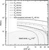 |
Fig. 4 Same as Fig. 1, except that αmin = 10−3 and clumps form at 5.6 × 10⁵ yr. |
| In the text | |
|
Fig. 5 Same as Fig. 2, except that αmin = 10−3 and clumps form at 2.8 × 10⁵ yr. The dash-dot-dotted line represents the semi-analytical estimate from Appendix A for the evolution of the radial positions of a clump forming at 3.0 × 10⁵ yr at 57 AU. |
| In the text | |
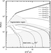 |
Fig. 6 Same as Fig. 3, except for αmin = 10−3. |
| In the text | |
|
Fig. 7 Dependence of clump migration on ω in disks with MMCC = 1 M⊙ and TMCC = 15 K. Using different line styles, we differentiate different ω values. Each pair of the lines with the same style represents the time evolution of the radial positions of the clumps forming at the inner and the outer boundary of the fragmentation region at t = 3.5 × 10⁵ yr (time when the collapse of the parent cloud core ends) in a protoplanetary disk with a specific ω. The pairs of the dotted, short-dotted, solid, short-dashed, and dashed lines represent the evolution of the radial positions of clumps forming in disks with ω = 1.5 × 10⁻¹⁴ s−1, 2.0 × 10⁻¹⁴ s−1 2.8 × 10⁻¹⁴ s−1 5.0 × 10⁻¹⁴ s−1 and 8.0 × 10⁻¹⁴ s−1 respectively. The other information is the same as Fig. 1. |
| In the text | |
|
Fig. 8 Effect of the early formation of the clump with different ω. This figure shows the time evolution of the radial positions of clumps forming at the same radius Rinit = 34 AU in different disks with different ω and the same MMCC = 1 M⊙ and TMCC = 15 K. The solid line represents the evolution of the radial position of a clump forming at i = 2.7 × 10⁵ yr in a disk with ω = 2.8 × 10⁻¹⁴ s−1 and the dashed line represents that of a clump forming at i = 1.8 × 10⁵ yr in a disk with ω = 5.0 × 10⁻¹⁴ s−1. The shaded regions indicate the fragmentation regions, which refer to when and where the fragmentation conditions are satisfied. |
| In the text | |
|
Fig. 9 Dependence of clump migration on TMCC in disks with MMCC = 1 M⊙ and ω = 2.8 × 10⁻¹⁴ s−1. Using different line styles, we differentiate different TMCC. Each pair of the lines with the same style represents the time evolution of the radial positions of the clumps forming at the inner and the outer boundary of the fragmentation region at t = tinfall in a protoplanetary disk with a specific TMCC. The pairs of the dashed, short-dashed, solid, short-dotted, and dotted lines represent the evolution of the radial positions of clumps forming in disks with TMCC = 10 K, 12 K, 15 K, 18 K, and 20 K, respectively. Other information is the same as Fig. 1. |
| In the text | |
|
Fig. 10 Dependence of clump migration on MMCC in disks with TMCC = 15 K and ω = 2.8 × 10⁻¹⁴ s−1. Using different line styles, we differentiate different MMCC. Each pair of the lines with the same style represents the time evolution of the radial positions of the clumps forming at the inner and the outer boundary of the fragmentation region at t = tinfall in a protoplanetary disk with a specific MMCC. The pairs of the dashed, short-dashed, solid, short-dotted, and dotted lines represent the evolution of the radial positions of clumps forming in disks with MMCC = 0.6 M⊙, 0.8 M⊙, 1.0 M⊙, 1.2 M⊙, and 1.5 M⊙, respectively. Other information is the same as Fig. 1. |
| In the text | |
|
Fig. A.1 Numerically calculated α as a function of R at t = 106 yr in protoplanetary disks with the parent cloud core properties: MMCC = 1 M⊙, TMCC = 15 K, and ω = 2.8 × 10⁻¹⁴ s−1. The solid and dashed lines represent α in disks with αmin = 10−4 and 10−3, respectively. |
| In the text | |
Current usage metrics show cumulative count of Article Views (full-text article views including HTML views, PDF and ePub downloads, according to the available data) and Abstracts Views on Vision4Press platform.
Data correspond to usage on the plateform after 2015. The current usage metrics is available 48-96 hours after online publication and is updated daily on week days.
Initial download of the metrics may take a while.