| Issue |
A&A
Volume 684, April 2024
|
|
|---|---|---|
| Article Number | A55 | |
| Number of page(s) | 19 | |
| Section | Astronomical instrumentation | |
| DOI | https://doi.org/10.1051/0004-6361/202348217 | |
| Published online | 04 April 2024 | |
Using multiobjective optimization to reconstruct interferometric data
II. Polarimetry and time dynamics
1
Departament d’Astronomia i Astrofísica, Universitat de València,
C. Dr. Moliner 50,
46100
Burjassot,
València,
Spain
e-mail: This email address is being protected from spambots. You need JavaScript enabled to view it.
2
Observatori Astrònomic, Universitat de València,
Pare Científic, C. Catedràtico José Beltrán 2,
46980
Paterna,
València,
Spain
3
Max-Planck-Institut für Radioastronomie,
Auf dem Hügel 69,
53121
Bonn (Endenich),
Germany
4
National Radio Astronomy Observatory,
1011 Lopezville Rd,
Socorro,
NM
87801,
USA
e-mail: This email address is being protected from spambots. You need JavaScript enabled to view it.
Received:
10
October
2023
Accepted:
22
January
2024
Abstract
Context. In very long baseline interferometry (VLBI), signals recorded at multiple antennas are combined to form a sparsely sampled virtual aperture with an effective diameter set by the largest separation between the antennas. Due to the sparsity of the sampled aperture, VLBI imaging constitutes an ill-posed inverse problem. Various algorithms have been employed to deal with the VLBI imaging, including the recently proposed multiobjective evolutionary algorithm by decomposition (MOEA/D) described in the first paper of this series.
Aims. Among the approaches to the reconstruction of the image features in total intensity from sparsely sampled visibilities, extensions to the polarimetric and the temporal domain are of great interest for the VLBI community in general and the Event Horizon Telescope Collabroration (EHTC) in particular. Based on the success of MOEA/D in presenting an alternative claim of the image structure in a unique, fast, and largely unsupervised way, we study the extension of MOEA/D to polarimetric and time dynamic reconstructions in this paper.
Methods. To this end, we utilized the multiobjective, evolutionary framework introduced for MOEA/D, but added the various penalty terms specific to total intensity imaging time-variable and polarimetric variants, respectively. We computed the Pareto front (the sample of all non-dominated solutions) and identified clusters of close proximities.
Results. We tested MOEA/D with synthetic data sets that are representative for the main science targets and instrumental configuration of the EHTC and its possible successors. We successfully recovered the polarimetric and time-dynamic signature of the ground truth movie (even with relative sparsity) and a set of realistic data corruptions.
Conclusions. MOEA/D has been successfully extended to polarimetric and time-dynamic reconstructions and, specifically, in a setting that would be expected for the EHTC. It offers a unique alternative and independent claim to the already existing methods, along with a number of additional benefits, namely: it is the first method that effectively explores the problem globally and compared to regularized maximum likelihood (RML) methods. Thus, it waives the need for parameter surveys. Hence, MOEA/D is a novel, useful tool to characterize the polarimetric and dynamic signatures in a VLBI data set robustly with a minimal set of user-based choices. In a consecutive work, we will address the last remaining limitation for MOEA/D (the number of pixels and numerical performance), so that MOEA/D can firmly solidify its place within the VLBI data reduction pipeline.
Key words: methods: numerical / techniques: high angular resolution / techniques: image processing / techniques: interferometric
Both first authors have contributed equally to this work.
© The Authors 2024
 Open Access article, published by EDP Sciences, under the terms of the Creative Commons Attribution License (https://creativecommons.org/licenses/by/4.0), which permits unrestricted use, distribution, and reproduction in any medium, provided the original work is properly cited.
This article is published in open access under the Subscribe to Open model. This email address is being protected from spambots. You need JavaScript enabled to view it. to support open access publication.
1 Introduction
For very long baseline interferometry (VLBI), multiple antennas in a radio-interferometric array are combined to achieve unmatched astronomical resolutions. The source is simultaneously observed by an array of radio antennas. As described by the van-Cittert-Zernike theorem (Thompson et al. 2017), the correlated products of the signals recorded by pairs of antennas are approximately the Fourier transform of the true sky brightness distribution with a Fourier frequency determined by the baseline separating the two antennas on the sky plane.
Image reconstruction deals with the problem of recovering the sky brightness distribution from these measurements. With a full sampling of the Fourier domain (commonly referred to as the u, υ plane), the original image could be retrieved by an inverse Fourier transform. However, due to the limited number of antennas and the limited amount of observing time, only a sparse subset of all Fourier coefficients is measured (the subset of all observed spatial Fourier frequencies is commonly referred to as the u, υ-coverage). Moreover, the observations are corrupted by additional thermal noise and instrumental calibration effects. Hence, the imaging problem is an ill-posed inverse problem.
In particular, global VLBI at mm-wavelengths pose a number of additional challenges: The number of antennas is small, the visibilities are less well calibrated (in fact, the phases are typically poorly constrained) and the signal-to-noise ratio (S/N) is worse compared to denser arrays operating at longer wavelengths. All in all, the reconstruction problem is insufficiently constrained and due to missing data and the need for self-calibration, it is also non-convex and possibly multimodal. Thus, the imaging relies on strong prior information, and a different selection of the regularization terms or prior distributions may produce significantly different image features.
CLEAN and its variants (Högbom 1974; Clark 1980; Bhatnagar & Cornwell 2004; Cornwell 2008; Rau & Cornwell 2011) are the de facto standard method for imaging since decades. However, recent years have seen the ongoing development of novel imaging algorithms for the global VLBI data regime, primarily inspired by the needs of the Event Horizon Telescope (EHT), in three main families: super-resolving CLEAN-based algorithms (Müller & Lobanov 2023b), Bayesian methods (Arras et al. 2021; Broderick et al. 2020b; Tiede 2022), and regularized maximum likelihood (RML) methods (Honma et al. 2014; Chael et al. 2016, 2018; Akiyama et al. 2017b,a; Müller & Lobanov 2022). These methods have been proven to be successful when applied to synthetic data (Event Horizon Telescope Collaboration 2019, 2022a) and in a wide range of frontline observations with the EHT (Event Horizon Telescope Collaboration 2019, 2022a; Kim et al. 2020; Janssen et al. 2021; Issaoun et al. 2022; Jorstad et al. 2023), the Global Millimetre VLBI Array (GMVA) observations (Zhao et al. 2022), and space-VLBI (Fuentes et al. 2023; Müller & Lobanov 2023a; Kim et al. 2023). One issue is that the image structure is only weakly constrained by the data and multiple solutions may fit the observed data; this is handled within these frameworks either via manual interaction in CLEAN (CLEAN windows, hybrid imaging, and self-calibration), a global posterior evaluation for Bayesian methods, or the combination of various data terms and regularization terms for RML methods. In particular, to overcome the limitation imposed by the sparse uυ-coverage and challenging calibration when observing at 230 GHz, the EHT has performed extensive and successful surveys exploring different parameter combinations. These were utilized to select a top-set of hyper-parameters, but have also served the purpose of providing synthetic data verification with a variety of source morphologies, with the aim of building confidence in the reconstructed images (in particular, for RML methods; see Event Horizon Telescope Collaboration 2019, 2022a). In this work, we focus on improving the top-set selection strategy.
Recently, we proposed a method known as MOEA/D, which presents an alternative claim (Müller et al. 2023, hereafter Paper I). MOEA/D approaches the image reconstruction by a multiobjective formulation similar in philosophy to parameter surveys that are common for RML methods (Paper I; Zhang & Li 2007). The nondominated, locally optimal solutions to the image reconstruction problem are identified by Pareto optimality. In this way, MOEA/D directly fits into the framework of a multimodal, nonconvex imaging problem, since it investigates all clusters of optimal features simultaneously (Zhang & Li 2007). As a particular benefit of MOEA/D, it is relatively fast and largely unsupervised. Compared to CLEAN, human supervision is no longer needed. Compared to Bayesian methods with manually chosen prior distributions and RML methods, MOEA/D has a small number of hyperparameters, it explicitly explores inherent degeneracies, and may not require parameter surveys (Paper I). An alternative strategy (i.e., to mapping the impact of various regularization assumptions by the Pareto front, thus reducing the number of critical free hyperparameters) would be to infer the priors or regularization terms together with the image structure as realized by resolve in a Bayesian framework (Arras et al. 2019), or by particle swarm optimization in an RML setting (Mus et al. 2024).
The VLBI community shows great interest in two extensions of the classical imaging problem: Polarimetric reconstructions (e.g., Lister et al. 2018; Kramer & MacDonald 2021; Event Horizon Telescope Collaboration 2021a,b; Ricci et al. 2022; Johnson et al. 2023) and time dynamic reconstructions (e.g., Johnson et al. 2017, 2023; Bouman et al. 2017; Lister et al. 2018, 2021; Satapathy et al. 2022; Wielgus et al. 2022; Farah et al. 2022). The option to recover polarimetric movies is of particular importance for the EHT and its possible successors (Johnson et al. 2023), but it does pose significant challenges (Roelofs et al. 2023). The imaging needs to deal with the relative sparsity of the array, various calibration issues at mm-wavelengths, super-resolution, polarimetry, and time dynamics simultaneously. Several algorithms and softwares that could deal specifically with time-dynamic reconstructions at the event horizon scales (Bouman et al. 2017; Johnson et al. 2017; Arras et al. 2022; Müller & Lobanov 2023a; Mus & Martí-Vidal 2024) or static polarimetry (Chael et al. 2016; Broderick et al. 2020b,a; Martí-Vidal et al. 2021; Pesce 2021; Müller & Lobanov 2023a) have been proposed. Recently, the potential of these approaches was demonstrated by Roelofs et al. (2023). However, the combined capability, namely, the reconstruction of polari-metric movies within one framework, remains a unique imaging capability for only a few algorithms, such as DoG-HiT (Müller & Lobanov 2023a).
In this manuscript, we build on the success of the recently proposed MOEA/D algorithm (Paper I) in presenting a fast and unsupervised alternative, independent of self-calibration (as long as self-calibration agnostic data functionals are used), to the already established imaging methods in total intensity and extend it both to polarimetric and time dynamic reconstructions in the same framework. In this spirit, this work contributes towards an automatic, unbiased reconstruction of polarimetric movies that is especially useful for the needs of the EHT and its planned successors.
2 VLBI measurements and polarimetry
The correlated signal of an antenna pair (the visibility 𝒱(u, υ)) is described by the van-Cittert-Zernike theorem (Thompson et al. 2017):
 (1)
(1)
This shows that the true sky brightness distribution, I(l, m), and the visibilies form approximately a Fourier pair. The harmonic coordinates, (u, υ), are determined by the baseline separating each antenna pair relative to the sky plane. Not all Fourier frequencies are measured, that is, the u, υ-coverage is sparse. Hence, the imaging process (i.e., recovering the sky brightness distribution from the observed visibilities) is an ill-posed inverse problem, since the codomain is only sparsely sampled. Furthermore, the visibilities are corrupted by calibration issues and thermal noise. We have to correct for these effects during imaging as well. The measured visibilities at a time, t, observed along one pair of antennas, i, j, are multiplied by station-based gain factors at each instant, t, 𝒢i,t, to correct direction-independent calibration effects, mathematically expressed as:
 (2)
(2)
with a baseline-dependent random noise term of Ni,j,t. Hereafter, we consider V, 𝒢, I, g, and N to be time-dependent, unless otherwise stated. To simplify the notation, we omit the t.
The polarized fraction of the light recorded at every antenna is splitted by polarization filters (either orthogonal linear, or right-handed and left-handed circular). These four channels per baseline (two per antenna) are combined in the four Stokes parameters: I, Q, U, V; here, I describes non-negative total intensity, Q, U linear polarization, and V the circular polarization. The Stokes parameters satisfy the following inequality:
 (3)
(3)
namely, the total intensity of polarized and unpolarized emission is always greater than the polarized intensity. In a similar process as the one used for Stokes I imaging, we can identify Stokes visibilities for the various Stokes parameters (Thompson et al. 2017):
 (4)
(4)
 (5)
(5)
 (6)
(6)
 (7)
(7)
where 𝓕 denotes the Fourier transform. We treat the Stokes visibilities as the “observable” for the remainder of this manuscript.
Preparing the discussion of leakage corruptions, and the corresponding calibration within MOEA/D, we also discuss the formulation by visibility matrices here. However, note that we will fit the Stokes visibilities directly with MOEA/D and not the coeherency matrices. For circular feeds, we arrange the polarized visibilities for an antenna pair i, j in the visibility matrix (Hamaker et al. 1996):
 (8)
(8)
For polarimetry, we have to deal with station-based gains and thermal noise in all bands. Additionally we have to deal with leakages and feed rotations in polarimetry. Gains are most easily represented by the Jones matrix (Thompson et al. 2017) for antenna i:
 (9)
(9)
and feed rotations by the matrix θ (Thompson et al. 2017):
 (10)
(10)
The leakage between the perpendicular polarization filters introduces cross-terms (Thompson et al. 2017):
 (11)
(11)
We denote the complete corruption by  . Then the observed visibility matrix Vi,j is:
 (12)
(12)
with thermal noise Ni,j.
3 MOEA/D
MOEA/D is a multiobjective optimization technique that was originally proposed in Zhang & Li (2007); Li & Zhang (2009) for multiobjective optimization problems in a general setting. The framework was adapted for VLBI imaging in Paper I. In Paper I, we connected the various objectives that are balanced against each other in a RML formulation of the imaging problem (i.e., the various data terms and penalizations) to the single objectives of a multiobjective problem formulation. In this way, MOEA/D explores all possible regularization parameter combinations simultaneously, and a lengthy parameter survey could be omitted, although the number of pixels is a crucial factor in the complexity of the problem. A new technique not as sensitive to the number of pixels based on particle swarm optimization is being developed Mus et al. (2024). Moreover, we introduced a more global search technique by the genetic algorithm in Paper I. In this section, we recall some of the basic concepts of MOEA/D. For more details, we refer to Paper I.
For MOEA/D, the imaging problem is reformulated as a multiobjective optimization problem, hereafter, “the problem” (Pardalos et al. 2017; Paper I):
 (MOP)
(MOP)
where ƒi : D → ℝ, i = 1 …, m are the single objective functionals, D is the decision space, and F : D → ℝn the vector-valued multiobjective optimization functional. For the minimization of F, we looked for the most optimal compromise solutions. A guess solution of x* ∊ D is called Pareto optimal or nondominated, if the further optimization in one objective automatically worsens the scoring in another objective functional, namely, if no point x ∊ D exists, such that ƒi (x) ≤ ƒi (x*), ∀i = 1, …, m and ƒj (x) < ƒj (x*) for at least one j = 1,…,m (Pardalos et al. 2017; Paper I). The set of all Pareto optimal solutions is called the Pareto front (Pardalos et al. 2017).
In Paper I, we chose the following modelization for Stokes I imaging:
 (13)
(13)
 (14)
(14)
 (15)
(15)
 (16)
(16)
 (17)
(17)
 (18)
(18)
 (19)
(19)
where Svis, Samp, Sclp, Scla are the reduced χ2-metrics with respect to the visibilities, amplitudes, closure phases, and closure amplitudes, respectively, while Rl1,Rl2, Rtv, Rtsv, Rflux, Rentr denote the l1−, l2−, total variation, total squared variation, compact flux, and entropy penalty terms. For more details on these terms, we refer to the more detailed discussion in Paper I.
The output of the MOEA/D is a sample of potential image features covering the decision space among the axes of all data terms and regularizers rather than a single image. Hence, the problem is high-dimensional limiting the number of pixels to achieve a sufficient numerical performance. Furthermore, the genetic algorithm, while exploring the parameter space globally, does not take into account gradient or hessian information, thus converges rather slow. These points are tackled in a companion effort (Mus et al. 2024) that replaces the genetic evolution by a hybrid approach and waives the limitation of a small number of pixels.
Some of these objectives have discrepancies. For instance sparsity in the pixel basis (promoted byRl1) and smoothness (promoted by Rtsv) are contradicting assumptions. In essence, this means that a single image that minimizes all objective functionals, fi, typically does not exist (Pardalos et al. 2017). For RML methods we achieve a potential, regularized reconstruction by balancing these terms with the proper, but initially unknown, weighting parameters α, β,… by a weighted sum minimization. For MOEA/D all the different weighting combinations are explored simultaneously and are approximated by the Pareto front (Zhang & Li 2007). Due to the aforementioned discrepancies between data terms and penalty terms and in between different penalty terms, the Pareto front divides into several clusters of solutions (Paper I). The number of disconnected clusters is larger, the weaker the image features are constrained, namely, for enhanced sparsity of the array and for self-calibration independent closure-only imaging (Paper I). The recovered image morphologies within one cluster vary only marginally. However, the recovered image features among several disconnected clusters vary significantly. We identify the independent clusters in the Pareto front by a friends-on-friends algorithm (for more details we refer to Paper I).
While all the nondominated solutions are explored simultaneously within the Pareto front, we have to deal with the problem to find the cluster of solutions that is objectively best. In Paper I, we argued that this could be done without the need for lengthy parameter surveys by a more automatized choice in a data-driven way. We proposed using the solution that has the highest number of close neighbors (i.e., the dominating cluster of solutions) or the cluster that is minimizing the (euclidean) distance to the ideal point (mimicking a least-square principle). In the application to synthetic data and to real data, it was the choice with the largest number of close neighbors that showed the best performance (Paper I).
Generally, it is challenging to compute the Pareto front analytically. Hence, the Pareto front is typically approximated by a sample of characteristic members (Pardalos et al. 2017). Several strategies exist to approximate the Pareto front. Most of these algorithms decompose the multiobjective optimization problem into a sample of single-objective problems either by the Tchebycheff approach, the boundary intersection method, or the weighted sum approach (Tsurkov 2001; Zhang & Li 2007; Xin-She & Xing-Shi 2019; Sharma & Chahar 2022). We applied the weighted sum approach in Paper I given its philosophical similarity to parameter surveys that are common in VLBI for RML methods (e.g., cf. Event Horizon Telescope Collaboration 2019, 2022a; Kim et al. 2020; Janssen et al. 2021; Zhao et al. 2022; Fuentes et al. 2023). In this way, the Pareto front approximates the set of images using parameter surveys. We introduced normalized weight arrays  that are related to the objective functionals f1, f2, …, fm in Paper I to reformulate (as a weighted sum) the multiobjective problem (MOP) into a sequence of single-objective optimization problems (Paper I):
 (20)
(20)
We note that there are two different weights. The weights α, β,… (which remain fixed during the running time of MOEA/D) and the weights λi (which we search over for Pareto optimal solutions). The weights α, β,… are commonly used to renormalize the regularization terms and data terms to a similar order of magnitude to help the convergence procedure. However, they do not affect the estimation of the Pareto front as long as the grid the weights λi is large and dense enough. Paper (for more details, see Appendix A in Paper I).
One particularly successful strategy to approximate the Pareto front by decomposition is the multiobjective evolutionary algorithm MOEA/D proposed in Zhang & Li (2007); Li & Zhang (2009). MOEA/D computes the Pareto front by a genetic algorithm. We started with a random initial population. The subsequent population is obtained by evolutionary operations, namely, by random mutation and genetic mixing. MOEA/D fits specifically well into the framework of VLBI imaging, since only parent solutions with similar weight combinations  are genetically mixed, namely: the algorithm keeps the diversity within the population Paper I (Zhang & Li 2007).
MOEA/D for VLBI combines several advantages. It is faster than complete parameter surveys for RML methods or exact Bayesian sampling schemes, provides an alternative claim of the image structure in an automatized (unsupervised) way. It also explores the image features with a more global search technique: via a randomized evolution in a multiobjective framework (Paper I). In conclusion, the dependence on the selection of regularization terms inherent to all RML imaging procedures is addressed effectively by a multiobjective, more global exploration of the possible solution space.
4 Modelization of the problem
4.1 Polarimetry
For polarimetry, we introduced the χ2 -fit to the linear polarized visibilities, 𝒱Q, 𝒱U, as an additional data term: Spvis. Although it may be a small extension to also include circular polarization in the set of objectives and recover circular polarization among the linear polarization, we omit to this extension. Recovering circular polarization requires a range of additional calibration steps, particularly of the R/L gain ratio that are typically not performed in self-calibration, but across multiple sources (Homan & Wardle 1999; Homan & Lister 2006).
Moreover, we used specifically designed polarimetric regularization terms inspired by the selection in Chael et al. (2016) and subsequently used by the EHT collaboration (e.g., Event Horizon Telescope Collaboration 2021a). In particular, we use the functionals, Rms, Rhw, Rptv, that will be presented in the following paragraphs.
First, we use the conventional KL polarimetric entropy (Ponsonby 1973; Narayan & Nityananda 1986; Holdaway & Wardle 1988; Chael et al. 2016) of an image, I, with respect to a prior image, Mi, (chosen to be a Gaussian with roughly the size of the compact flux region):
 (21)
(21)
Here mi denotes the fraction of linear polarization in pixel, i, while Rhw favors images of N pixels with fractional polarization, m, of less than one.
The second regularizer, Rms, extends the concept of the entropy to the polarized image:
 (22)
(22)
We note that Rms diverges to negative infinity if the polarization fraction approaches zero. To avoid this, we actually used max(Rms, −ɀ) as the regularization term. Here, ɀ is a real number that has been found as the smallest scoring Rms(x) in the Pareto front that has not diverged. Finally, we utilized the polarimetric counterpart of the total variation regularizer (Chael et al. 2016):
 (23)
(23)
where we used the complex realization of the linear polarized emission P = Q + iU to note down the total variation for Q and U in a compact form.
In conclusion, the resulting multiobjective problem consists of the single functionals:
 (24)
(24)
 (25)
(25)
 (26)
(26)
 (27)
(27)
4.2 Dynamics
The philosophy behind time dynamic imaging is as follows: We cut the full observation into r keyframes where, for a given time window, where all frames satisfy the condition that there is at least one visibility observed. The visibilities of one frame are:
![Mathematical equation: ${{\cal V}^l} = \left\{ {{\cal V}\,\,{\rm{for}}\,\,t \in \left[ {{t_l} - {\rm{\Delta }}{t_l}/2,{t_l} + {\rm{\Delta }}{t_l}/2} \right]} \right\},l \in [1,r],$](/articles/aa/full_html/2024/04/aa48217-23/aa48217-23-eq32.png) (28)
(28)
where tl is the observing time and ∆tl is a frame-dependent scalar that determines its duration. For each l, the associated data set 𝒱l produces an “image keyframe”. The model will have a total of r × N2 parameters (i.e., r images of N2 pixels each). Now, we naturally extend the data terms and penalty terms to a time-series, for instance, by:
 (29)
(29)
where p is a time-series of images (i.e., a movie). We proceed analogously for all the other data terms and regularization terms.
In Paper I, we constructed the problem (MOP) using seven functionates including l2-norm (Rl2), l1-norm (Rl1), total variation (TV), and total squared variation (TSV)(Rtv, Rtsv), flux modeling (Rflux), and the entropy (Rentr) and standard visibility and closures data terms (Svis, Samp, Sclp, Scla). The detailed descriptions of each regularizer can be found in the referenced paper.
To extend this problem to include dynamics, we considered a new objective, namely: ƒngMEM, the ngMEM regularization term defined by Mus & Martí-Vidal (2024) acting on a time-series of images  :
:

where j, k ∊ {1, 2,…, r} denote the frame in the time-series, µngMEM is a hyper-parameter and
 (30)
(30)
Here, tj denotes the times of the associated keyframe j. This functional seeks the most constant dynamic reconstruction (or movie hereafter) which still fits into the data (Mus & Martí-Vidal 2024).
The ngMEM uses the Shannon entropy from Shannon (1949) without imposing any a priori model to ensure a uniform distribution in both brightness and time for a time-series of such frames. Therefore, it is a conservative approach, since any change in contrast will contribute to the increment of the entropy.
The two parameters µngMEM1 and π are used as regularizers and must be explored. Also, π, the “time memory” has a minor effect, while µngMEM, the “time weight”, must be carefully selected. Therefore, µngMEM should be investigated using MOEA/D. Finally, C is just a floor that should be small to avoid extremely large values or not-a-number errors for the logarithm.
We can solve this problem of dynamic imaging (i.e., find the set of image keyframes that optimally fit the data) by using the following formalism.
 (31)
(31)
 (32)
(32)
 (33)
(33)
 (34)
(34)
 (35)
(35)
 (36)
(36)
 (37)
(37)
 (38)
(38)
4.3 Dynamic polarimetry
Ultimately, the fusion of polarimetry regularizers with ngMEM offers a potent approach for the retrieval of polarimetric evolution. Given the inherent intricacies of this challenge, only a few algorithms possess the capability to address it. In particular, the only RML-like algorithm that is currently able to do so is DoG-HiT Müller & Lobanov (2023a). The Bayesian algorithm resolve Arras et al. (2019, 2021) has the potential to also recover dynamic polarimetry, although no publication to date has been done in that direction.
The modelization of the problem within the framework of MOEA/D is notably straightforward. In principle this could be achieved in the most consistent way by combining Eqs. (24)–(27) with Eqs. (31)–(37) by adding the polarimetric objectives to every single scan and solving for total intensity and polarization at the same time. However, the problem becomes rapidly high-dimensional and complex to solve, particularly when exploring the range of possible solutions the Pareto front. In particular, the complexity of the MOEA strategies ranges between  and
and  (Curry & Dagli 2014), with O being the asymptotic upper bound. The population size is the number of weight combinations drawn from an equidistant grid with overall sum 1, that is, np = binom(no + ng − 1, ng), where ng is the grid size. Current work is ongoing to achieve a better scaling by a grid-free evolution of the weights (Mus et al. 2024).
Moreover, since gains and d-terms are not part of the forward model, an application in practice is naturally limited to a hierarchical approach: solve for the d-terms and gains from the static image (with a subsequent refinement with the movie in total intensity first) before proceeding to a full polarimetric movie reconstruction.
Therefore, we split the strategy into several steps. First, we solved for the dynamics in total intensity as described above (step 1). Second we calculated a static polarimetric image as described above (step 2). Third, we cut the observation into keyframes and solved the polarimetric imaging at every keyframe independently with MOEA/D, initializing the population with the final population of the static polarization step (step 2) and assuming the Stokes I image from the time-dynamic exploration (step 1). This strategy resembles the strategy that was also applied in Müller & Lobanov (2023a) for DoG-HiT, one of the few algorithms that already has the capability for dynamic polarimetry.
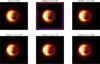 |
Fig. 1 Clustered images for simulated Sgr A* polarimetric model using the EHT 2017 array at 230 GHz and. The preferred cluster by the largest number of representants is indicated by a red box, the one preferred by the closest distance to the ideal point by a blue box. Vertical lines represent the EVPA. |
4.4 Pareto fronts
In case of polarimetry, the Pareto front is a four-dimensional hypersurface (four objective terms). As for total intensity, the Pareto front divides into several disjunct clusters due to conflicting assumptions of several regularization terms. We examined the Pareto front in the same way as described in Paper I, that is, we identified the clusters of solutions in the scoring by a friends-on-friends algorithm. Afterwards, we evaluated the representative solutions of every cluster by its number of close neighbors and by the distance to the ideal, for more details see Paper I. For special clusters, namely, for the clusters that present overfitted data, the polarization fraction accumulates at the edges of the interval [0,1]. In this case, the regularizer approaches negative infinity. We explicitly excluded these clusters for the finding of the objectively best solution.
In the dynamic case, the dimensionality of the Pareto front is 8. The resulting “Pareto movies” are defined by the action of the different objectives on the recovered movies defined by the frames obtained. Finally, the Pareto front obtained solving the dynamic polarimetric problem is composed by the two disjoint Pareto fronts defined above.
5 Verification on synthetic data in EHT+ngEHT array
5.1 Array configurations and problem framework
The self-consistent reconstruction of polarimetric dynamics at the event horizon scales is one of the major goals of the EHT and its planned successors (Johnson et al. 2023; Roelofs et al. 2023). Hence, to maintain consistency with the analysis presented in Müller et al. (2023), here, we studied two array configurations for the remainder of this manuscript. On one hand, we study the configuration of the EHT observations of SgrA* in 2017 at 230 GHz (Event Horizon Telescope Collaboration 2022b). On the other hand, we study a possible EHT + ngEHT configuration that was also used within the ngEHT Analysis challenges (Roelofs et al. 2023), including ten additional stations at 230 GHz, a quadrupled bandwidth and an enhanced frequency coverage. For consistency with Paper I, we have solved the different MOPs using 256 pixels.
5.2 Polarimetry
To demonstrate the capabilities of MOEA/D in the polarimetric domain, we use a synthetic data source out of the ehtim software package (Chael et al. 2016, 2018) that was previously used in Müller & Lobanov (2023a) for synthetic data tests as well. The ground truth image is plotted in the upper left panel of Fig. 1. The model mimics the typical crescent-like black hole shadow of Sgr A* in total intensity with a highly linear polarized structure.
We show our reconstructions in the same way as we did in Paper I. The non-dominated solutions in the final, evolved population of the Pareto front form disconnected clusters of solutions. The variety of the recovered structure within one cluster is small, however, the variety in the recovered image structures between different clusters of reconstructions is significant. We present in Fig. 1, one representant of each cluster of solutions (the accumulation point) in comparison to the true image structure. The existence of multiple clusters with a single particle starting point already hints that MOEA/D at least partially overcame local convexity and searched the solution space globally independent of the starting point.
For the polarimetric reconstruction, we fixed the Stokes I reconstruction since we suppose datasets need to be d-term calibrated (however note that if d-terms are lower than 10%, imaging algorithms have stronger effects on the reconstruction than the d-terms; Martí-Vidal & Marcaide 2008), and only solved for linear polarization with MOEA/D. Moreover, this strategy mimics the strategy of splitting the RML parameter surveys into a total intensity and polarimetry part as was applied by the EHT. We initialized the initial population with images with constant electric vector position angle (EVPA) at a constant polarization fraction of 1% across the whole field of view. Rather than use the Stokes parameters Q, U, we equivalently modeled the linear polarization by the linear polarization fraction m and the mixing angle χ, as follows:
 (39)
(39)
This turns out to be beneficial since any inequality (Eq. (3)) is automatically satisfied by imposing 0 ≤ m ≤ 1 (assuming small Stokes V) during the genetic evolution. We recover some unde-sired solutions when the weighting favors Rms as this term promotes small polarization fraction approaching m = 0, as shown in Fig. 1). However, these solutions are disfavored as they are at the edge of the Pareto front and are not selected by neither of the selection heuristics. Specifically, we cannot create spurious polarimetric signals outside of the total intensity contours. MOEA/D evolves the population of solutions by genetic operations, namely, by genetic mixing and random mutation. For latter step, it is beneficial for the numerical performance to rescale all guess arrays (i.e., m and χ) such that the resulting values are of order of 1, we refer to Paper I for more details on the numerical performance.
Out of the clusters of solutions presented in Fig. 1 one (cluster 0) recovers the polarization fraction well. The EVPA pattern, particularly the small-scale perturbation towards the south-east of the ring, is recovered well. Cluster 0 is both strongly preferred by the absolute χ2 (i.e., it is the cluster that fits the data best) as also by the accumulation point criterion that we proposed in Paper I (i.e., it is the cluster with the largest number of neighbors, hence, it is the most “common” one).
To verify that MOEA/D reconstructions performs well for a wider range of EVPA structures on such a challenging data set as the EHT observations, we carried out a number of additional tests with an artificial ring image and a constant EVPA pattern, a toroidal magnetic field, a radial magnetic field and a vertical magnetic field, see Figs. 2, 3, 4, and 5 respectively. For each case, we show the respective best solutions selected by the accumulation point criterion (right columns) and the real model (left columns). Bottom rows show model and solution convolved with a 20 µas beam (represented as a white circle in the plot). The reconstruction of the overall pattern is successfully recovered in all four convolved cases; however, we note how super-resolution scrambles the pattern. In conclusion, we can differentiate various magnetic field configurations by the MOEA/D reconstructions of EHT like data.
Here, we go on to study how the reconstruction improves with an improved array. We present the same GRMHD simulated reconstruction observed with a ngEHT configuration in Fig. 6. Due to the larger number of visibilities, the observation is more constrained. The reconstruction within the preferred cluster(cluster 0) improves, particularly with respect to the total polarization fraction. Interestingly, the non-preferred clusters (at the edge of the parameter space) still exist, resembling the weight combinations that overweight Rms, but are strongly discouraged by investigating the properties of the Pareto front. For more details regarding tools to investigate the Pareto front, for instance, by looking for disjoint clusters, accumulation points and the solution closest to the optimum, we refer to Paper I.
Finally, we studied the reconstruction performance in the presence of more realistic data corruptions as they may be expected in real data sets. For this, we introduced gain errors (i.e., the need for self-calibration) and leakage errors (i.e., the need to calibrate d-terms) into the synthetic observation with the ngEHT coverage. We added d-terms randomly at all sites with a an error of roughly 5% for dr and dl, independently, and gains with a standard deviation of 10%. First we performed a Stokes I reconstruction with MOEA/D. As described in Paper I, this reconstruction uses the closure quantities only; hence, it is is less prone to the gain uncertainties. We selected the best image based on the accumulation point criterion and self-calibrated the data set with this Stokes I image. In the next step, we held the total Stokes I structure constant and recovered the linear polarization. While a common reconstruction (and calibration) of total intensity and polarized structures is desired – and indeed realized, for instance, in state-of-the-art Bayesian frameworks (Broderick et al. 2020b; Tiede 2022), we skipped this approach to avoid an overly high dimensionality due to the large number of multiobjective functionals that we would need to combine. We calculated an initial guess for the polarimetric structure by ehtim with an unpenalized reconstruction, similar in philosophy to the initial guesses that are typically used for DoG-HiT (Müller & Lobanov 2022). This initial guess is used to perform an a-priori d-term calibration and to initialize the population for MOEA/D. We used ehtim for the final d-term calibration and then imaging with MOEA/D.
In Fig. A.1, we show the correlation of MOEA/D obtained dterms and the ground truth. We can qualitatively see how we recover a close correlation (dashed blue line), implying that MOEA/D solution has dterms similar to the ground truth. In Appendix C, the specific value of the dterm for the true case and the solution for every site can be found.
MOEA/D approximates the overall structure during the first few iterations, evolving the front towards more fine-structure in later iterations over time. Hence, it is a natural approach to use imaging and calibration in an alternating mode: We evolved the initial population by MOEA/D for some iterations, use the current best guess model to calibrate d-terms, and rerun MOEA/D with the old population as an initial guess (i.e., we let the population adapt to slightly varied objectives in an evolutionary way). We iterated this procedure three times. The corresponding reconstruction result is shown in Fig. A.2. The overall structure of the Pareto front is similar to the fronts presented before in Figs. 1 and 6 with one dominating cluster. We recovered the structure in the EVPAs successfully, however, we would like to highlight that the linear polarization fraction ended up underestimated. This may be a consequence of the self-calibration procedure since an initial guess with a smaller polarization fraction than the true one was used.
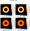 |
Fig. 2 Simulated ring-like source with constant vertical EVPA using EHT 2017 array. Left panel: ground truth. Right panel: Preferred image (solution) recovered with MOEA/D image. Bottom row: super-resolved structures. Bottom row: images convolved with 20 µas beam shown in white. Vertical lines represent the EVPA and their color is the level of the polarization fraction. The color map for the brightness of the source is different to the one of the EVPAs. |
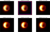 |
Fig. 6 Cluster of images obtained with MOEA/D for a simulated polarimetric Sgr A* model using EHT+ngEHT array configuration at 230 GHz. |
5.3 Dynamics
The capability of recovering dynamic reconstructions using MOEA/D has been tested using two independent synthetic pieces of data simulating a SMBH with an accretion disk based on general relativity magnetohydrodynamics (GRMHD) models. The first data set (the simpler one) is based on the one presented in Johnson et al. (2017), Shiokawa (2013), and the data were shared by private communication. This data only contains Stokes I information. We call this data MJ2017. Similar to Appendix A of Paper I, we performed a small survey to find values that better show numerical performance for the µngMEM initial value. We found that 1 is a good starting value.
The second synthetic data, called the CH3 set, is the one given for the Challlenge 3 presented in Roelofs et al. (2023)2. The synthetic data of this last dataset is dynamically polarized, namely, the intrinsic polarization structure of the source varies along the observation. Therefore, we show an example of a joint polarimetric and dynamic reconstruction; thus we can see how MOEA/D solves for polarimetric movies and dynamics are not limited to Stokes I.
To assess the performance of MOEA/D in dynamic reconstruction, we replicated the experiment conducted by Johnson et al. (2017), based on a GRMHD simulation of a black hole. More details can be found in the cited paper and in Shiokawa (2013). Specifically, we reconstructed a similar keyframes presented in Fig. 4 of their work, which correspond to time instances at 16:00 UTC, 00:43:26 UTC and 06:29:27 UTC. These keyframes represent subsets of antennas observed within the EHT 2017 array configuration. The first keyframe involves approximately four antennas, the second approximately five antennas, and the final one only has approximately two antennas. The differing numbers of baselines between these keyframes render the reconstruction of a continuous movie through snapshot imaging unfeasible. A comprehensive comparison between the performance of ngMEM and the regularizers proposed by Johnson et al. (2017) in this specific scenario is detailed in Mus & Martí-Vidal (2024).
To generate a comparable movie, we initially constructed a tentative movie using the constrained ngMEM. Subsequently, we flagged all visibilities corresponding to the aforementioned timestamps. Employing the “guess movie” as an initial point of our algorithm, we executed MOEA/D to explore the neighborhood of the movie.
We present our reconstruction results in Fig. A.8. Despite the extreme sparsity of the observation, MOEA/D successfully captures the fine crescent structure for all three snapshots. First column of the figure represents the simulation with infinite resolution. The middle column shows the simulation convolved with the beam of the EHT ~ 20 µarcsec (indicated as a with circle), and the third column shows the one representative solution of the MOEA/D convolved with the same beam. In Fig. B.1, the Pareto front for each of the keyframes is presented.
The obtained results exhibit a performance deficit compared to those demonstrated in Mus & Martí-Vidal (2024). This discrepancy can be attributed to the inherent loss of cross-talk information between frames in our methodology. The cited paper uses a Hessian modeling, which encodes the correlation information of the frames. Therefore, a better reconstruction can be done. However, it is important to acknowledge that this choice restricts the optimization process to a local scope, potentially resulting in the loss of the possibly inherent multimodal nature of the problem.
5.4 Dynamic polarimetry
We tested the capability to carry out dynamic polarimetry with a synthetic data set that is based on the ngEHT analysis challenges (Roelofs et al. 2023). Specifically, we used the SGRA_RIAFSPOT model from the third ngEHT Analysis challenge3. The ground truth movie of Sgr A* is a RIAF model (Broderick et al. 2016) with a shearing hotspot (Tiede et al. 2020) inspired by the observations of GRAVITY Collaboration (2018). For more details on the simulation we refer to Roelofs et al. (2023); Chatterjee et al. (2023). We show the ground truth movie in Fig. A.3. For the plotting, we regridded every frame to the field of view and pixel size that was adapted for MOEA/D, namely, we represent the image structure by 10 µas pixels. We observed the movie synthetically by the possible EHT+ngEHT configuration specified in Roelofs et al. (2023). This configuration consists of all current EHT antennas and ten additional antennas from the list of proposed sites by Raymond et al. (2021). We synthetically observe the source in a cadence with scans of 10 min of observation and 2 min gaps between integration times, as was done already in Müller & Lobanov (2023a). We added thermal noise, but assume a proper gain and d-term calibration.
We show the recovered reconstruction in Fig. A.4. The polarimetric movie was recovered with snapshots of 6 min in the time-window with the best uυ-coverage. For better comparison we show single snapshots in Figs. A.5–A.7. The ring-like image of the black hole shadow is successfully recovered at every keyframe with varying brightness asymmetry. Moreover, we successfully recover some hints for the dynamics at the event horizon in the form of a shearing hotspot, albeit the large pixel size limits the quality of the reconstruction. The overall EVPA pattern (orientation and strengths) is very well recovered in all keyframes. The dynamics of the EVPA pattern is well recovered as well as demonstrated for example by the well recovered enhanced polarization fraction towards the shearing hotspot in the top-right of Fig. A.6 and the top-left of Fig. A.7.
5.5 Quantitative evaluation
To perform a quantitative evaluation of the similarity among the MOEA/D polarimetric dynamic reconstruction, we show this via different figures of merit: the angular distribution of the reconstruction, the normal cross-correlation in total intensity (see, for instance Farah et al. 2022), and β2 to compare the EVPA pattern. First, it is worth noticing that since ngMEM allows us to capture the evolution in every integration time, the comparison can be done in every frame (all integration times).
Regarding the Stokes I evolution, we present our results in Figs. A.9 and A.10. The first plot shows the angular brightness distribution in each integration time for both the model and reconstruction. The second plot compares the maximum bright peak of the phase of the ground truth and the model. This plot also shows the nxcorr frame-wise performing the worst at the beginning of the experiment (as seen also with β2) and improving over the course of the observation.
In Figs. A.11 and A.12, we show the β2 amplitude (first figure) and phase (second figure) evolution during the experiment. The parameter β2 is used to describe the polarimetric signature in the EHT observations, as introduced by Palumbo et al. (2020). Because the use of closures during the optimization process, the absolute position of the source was lost. Therefore, in order to compare with the real source, we aligned each keyframe of the reconstruction with the model by shifting the baricenter of the image to the north, east, south, and west by one pixel. Errors bars in the β2 reconstruction are the standard deviations by these shifts, representing the possible errors obtained by image alignment. In both amplitude and phases we see a similar and congruent trend between the true solution and the recovered solution. However, the first keyframes recover the worst β2, which is consistent with the findings with respect to the total intensity. We note that the first scans are also the scans in which the source is evolving the fastest and, thus, the scans are more challenging to recover.
We show in Fig. A.13 the net polarization (for instance Event Horizon Telescope Collaboration 2021c) evolving over time. MOEA/D performs quite well in recovering the correct polarization fraction at all times, even in the rapidly evolving first part of the evolution, where MOEA/D had more issues with finding the twistiness of the pattern (as indicated by β2). The potential of MOEA/D to recover the correct polarization fraction with the EHT+ngEHT coverage is already shown in Fig. 6. It is noteworthy to consider that while we spotted an underestimated polarization fraction for leakage-corrupted data, the time-dynamic (but fully calibrated) reconstruction with the same array does not show this tendency.
6 Summary and conclusions
Imaging reconstruction of interferometric data is a challenging ill-posed problem, particularly when dealing with very sparse uυ-coverage, as is often the case in global VLBI observations. These challenges are amplified when working with polarimetric data or attempting to capture the dynamic behavior of the source. They become even more complex when reconstructing the evolving polarimetric data.
On the one hand, while static polarimetry imaging has been extensively studied in the past (Ponsonby 1973; Narayan & Nityananda 1986; Holdaway & Wardle 1988; Coughlan & Gabuzda 2013; Chael et al. 2016), solving the problem of polarimetric multiobjective imaging remains an open challenge. On the other hand, the intricacies presented by rapidly evolving sources, such as the case of Sgr A* (Event Horizon Telescope Collaboration 2022a), have prompted the VLBI community to develop innovative algorithms capable of effectively addressing variability concerns. The inherent limitations of snapshot imaging due to restricted coverage and the potential loss of information resulting from temporal averaging highlight the necessity for the formulation of functionals that can efficiently mitigate such information loss.
In this study, we have extended the MOEA/D algorithm, which was initially introduced in Paper I, to tackle the challenges associated with imaging Stokes I, Q, and U parameters, fractional polarization (m), and dynamics. This enhanced iteration of MOEA/D showcases its efficiency in reconstructing both static and dynamic interferometric data.
In this work, we first introduce the modelization of MOEA/D for static polarimetry and dynamic Stokes I by incorporating the relevant functionals in Eqs. (24)–(27) for the polarimetry and ngMEM (Mus & Martí-Vidal 2024), as well as Eq. (37) for the dynamic recovery. Subsequently, we tested our algorithm using synthetic data for both scenarios: polarimetry and dynamics. Finally, utilizing synthetic data from EHT+ngEHT, we demonstrated how MOEA/D excels in recovering polarimetric sequences, a capability possessed by only a select few algorithms.
The main benefits of MOEA/D for VLBI imaging are as follows. Opposed to classical RML and Bayesian techniques MOEA/D self-consistently explores imaging problem globally with multiple image modes, namely: the issue of missing data for sparsely sampled VLBI observations. In this way, MOEA/D presents a robust, alternative claim of the image structure. Moreover, due to the full exploration of the Pareto front, parameter surveys are not needed to establish the estimate of the image, thus MOEA/D is a significant step towards an effectively unsu-pervised imaging procedure. It is noteworthy that MOEA/D handle the non-negativity by imposing bounds on the image structure during the genetic operations rather than using the lognormal transform for the functional evaluations or adding lower-bound-constraints. In the same way, m is constrained to be in [0, 1] during the genetic evolution process. However, solutions accumulating at the edges of this interval are common due to the polarimetric entropy and the random nature of the genetic algorithm.
In conclusion, in this set of two papers, we have shown how MOEA/D is able to recover static and dynamic imaging algorithm, for Stokes I and polarimetry, effectively mitigating some of the limitations associated with the current state-of-the-art RML methods. Its flexibility and proficiency in recovering Pareto optimal solutions render this algorithm an invaluable tool for imaging reconstruction of interferometric data, catering to both current and next-generation telescopes.
One remaining weakness of MOEA/D is its current limitation to a small number of pixels (256 in this set of two papers). To overcome this problem, an alternative formulation is done in Mus et al. (2024), in which the evolutionary search algorithm is only used to find the optimal combination of weights. The authors develop a swarm intelligence strategy to find the optimal weights associated to the RML problem, regardless of the quality of the obtained image. Once the optimal weights are found, the corresponding image is (by definition) a member of the Pareto front and, thus, a valid and desirable solution. Then an optimal image can be found using a local search algorithm, as L-BFG-S (Liu & Nocedal 1989) imposing a correlation between close pixels (via a quasi-Hessian). The resulting image is called “PSO reconstruction.”
Acknowledgements
A.M. and H.M. have contributed equally to this work. This work was partially supported by the M2FINDERS project funded by the European Research Council (ERC) under the European Union’s Horizon 2020 Research and Innovation Programme (Grant Agreement No. 101018682) and by the MICINN Research Project PID2019-108995GB-C22. A.M. and I.M. also thank the Generalitat Valenciana for funding, in the frame of the GenT Project CIDEGENT/2018/021 and the Max Plank Institut fur Radioastronomie for covering the visit to Bonn which has made this possible. H.M. received financial support for this research from the International Max Planck Research School (IMPRS) for Astronomy and Astrophysics at the Universities of Bonn and Cologne. Authors acknowledge Michael Johnson for sharing via private communication their synthetic data. Software availability: We will make our imaging pipeline and our software available soon in the second release of MrBeam (https://github.com/hmuellergoe/mrbeam). Our software makes use of the publicly available ehtim (Chael et al. 2016, 2018), regpy (Regpy 2019), MrBeam (Müller & Lobanov 2022, 2023b,a), and pygmo (Biscani & Izzo 2020) packages.
Appendix A Additional figures
In this Appendix, we include the figures mentioned in the main text.
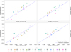 |
Fig. A.1 D-terms comparison between the ground truth simulated and that recovered by MOEA/D using closure-only of the source showed in Fig. A.2. Different sites are represented by different colors and markers explained in the legend. The dashed blue lines indicates a perfect correlation. The closer the derms to the line the better correlation between the terms. Top row: DR dterms (real and imaginary part from left to right). Bottom row: DL dterms. |
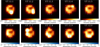 |
Fig. A.3 True movie of the ngEHT Challenge 3 synthetic data (Roelofs et al. 2023). Observation has been divided in 10 keyframe, each of them has been regridded to the MOEA/D resolution, namely, to 10 µas pixels. EVPA are represented as lines and their corresponding polarization fraction appears as color map: the bluer, the stronger m. The intensity of the source is represented by other color map. |
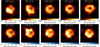 |
Fig. A.4 Recovered movie of the ngEHT Challenge 3 synthetic data (Roelofs et al. 2023). Each keyframe (which corresponds to exactly the same keyframes depicted in A.3) has been regridded to the MOEA/D resolution, namely, to 10 µas pixels. |
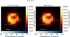 |
Fig. A.5 Single keyframe at UTC 11.3 recovered from the third ngEHT analysis challenge, with the ground truth image on the left and the recovered keyframe in the right panel. The keyframe has been regridded to the MOEA/D resolution: 10 µas pixels. |
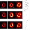 |
Fig. A.8 Comparison reconstructions of Johnson et al. (2017) method and MOEA/D for the different uυ-coverages of each keyframe. The color scale is linear and is consistent among different times, but is scaled separately for each case, based on the maximum brightness over all frames. The normal cross-corrleation (nxcorr) value between the recovered and the convolved model can be found in the bottom corner of the reconstructed images. A frame-wise comparison can be found in Mus (2023). |
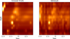 |
Fig. A.9 Phase diagrams as presented in Mus & Martí-Vidal (2024). Horizontal axis represent the time (frames) and vertical axis the angle. Keyframes are linearly interpolated in every integration time. Left panel: Model corresponding to the dynamical movie. Right panel: Recovered movie. We can see how MMOEA/D is able to recover the hotpsot movement (brightest lines). |
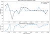 |
Fig. A.10 Similar to Fig. A.9 but only giving the peak brightness angle versus time (top). The lack line is the ground truth and blue line the recovered solution. In the bottom panel, nxcorr is given for every frame. |
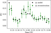 |
Fig. A.11 Amplitude, β2, of the model (black dots), of the reconstruction (green dots), and the complex norm of their difference (blue dashed lines). |
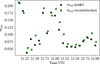 |
Fig. A.13 The net polarization as a function of time. |
Appendix B Pareto fronts of the MJ2017 data
In this Appendix, we present the three Pareto fronts, each corresponding to a keyframe, concerning the MJ2017 dataset detailed in Sect. 5.3.
The keyframe solutions shown in Fig. A.8, are the favored cluster (indicated by the red box) of the three Pareto fronts.
The sparsity observed in the uυ-coverage across each snapshot is responsible for the significant diversity observed in the solutions. It is interesting to observe that, in all three cases, only a limited number of clusters exhibit a ring-like structure. Nevertheless, it is worth highlighting that ring structures are the predominant and highly probable solutions. In fact, all of the selected solutions, particularly the most recurrent ones, conform to ring-like geometry.
Lastly, from the bottom right panel, we can deduce that better movie reconstructions require higher weight for the time entropy, as expected.
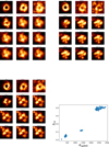 |
Fig. B.1 Pareto fronts for the first (top left), second (top right) and third (bottom left) keyframe for the MJ2017 data. Bottom right panel shows the µngMEM dependence with respect to the data fidelity term. |
Appendix C Dterm values
In this appendix, we give the specific dterms values of Fig. A.1 in Tab. C.1.
Dterms for the MOEA/D solution and ground truth.
References
- Akiyama, K., Ikeda, S., Pleau, M., et al. 2017a, AJ, 153, 159 [NASA ADS] [CrossRef] [Google Scholar]
- Akiyama, K., Kuramochi, K., Ikeda, S., et al. 2017b, ApJ, 838, 1 [NASA ADS] [CrossRef] [Google Scholar]
- Arras, P., Frank, P., Leike, R., Westermann, R., & Enßlin, T. A. 2019, A&A, 627, A134 [NASA ADS] [CrossRef] [EDP Sciences] [Google Scholar]
- Arras, P., Bester, H. L., Perley, R. A., et al. 2021, A&A, 646, A84 [NASA ADS] [CrossRef] [EDP Sciences] [Google Scholar]
- Arras, P., Frank, P., Haim, P., et al. 2022, Nat. Astron., 6, 259 [NASA ADS] [CrossRef] [Google Scholar]
- Bhatnagar, S., & Cornwell, T. J. 2004, A&A, 426, 747 [NASA ADS] [CrossRef] [EDP Sciences] [Google Scholar]
- Biscani, F., & Izzo, D. 2020, J. Open Source Softw., 5, 2338 [NASA ADS] [CrossRef] [Google Scholar]
- Bouman, K. L., Johnson, M. D., Dalca, A. V., et al. 2017, arXiv e-prints [arXiv:1711.01357] [Google Scholar]
- Broderick, A. E., Fish, V. L., Johnson, M. D., et al. 2016, ApJ, 820, 137 [Google Scholar]
- Broderick, A. E., Gold, R., Karami, M., et al. 2020a, ApJ, 897, 139 [Google Scholar]
- Broderick, A. E., Pesce, D. W., Tiede, P., Pu, H.-Y., & Gold, R. 2020b, ApJ, 898, 9 [Google Scholar]
- Chael, A. A., Johnson, M. D., Narayan, R., et al. 2016, ApJ, 829, 11 [Google Scholar]
- Chael, A. A., Johnson, M. D., Bouman, K. L., et al. 2018, ApJ, 857, 23 [Google Scholar]
- Chatterjee, K., Chael, A., Tiede, P., et al. 2023, Galaxies, 11, 38 [NASA ADS] [CrossRef] [Google Scholar]
- Clark, B. G. 1980, A&A, 89, 377 [NASA ADS] [Google Scholar]
- Cornwell, T. J. 2008, IEEE J. Selected Top. Signal Process., 2, 793 [NASA ADS] [CrossRef] [Google Scholar]
- Coughlan, C. P., & Gabuzda, D. C. 2013, Eur. Phys. J. Web Conf., 61, 07009 [NASA ADS] [CrossRef] [EDP Sciences] [Google Scholar]
- Curry, D. M., & Dagli, C. H. 2014, Procedia Comput. Sci., 36, 185 [NASA ADS] [CrossRef] [Google Scholar]
- Event Horizon Telescope Collaboration (Akiyama, K., et al.) 2019, ApJ, 875, L4 [Google Scholar]
- Event Horizon Telescope Collaboration (Akiyama, K., et al.) 2021a, ApJ, 910, 48 [CrossRef] [Google Scholar]
- Event Horizon Telescope Collaboration (Akiyama, K., et al.) 2021b, ApJ, 910, L43 [CrossRef] [Google Scholar]
- Event Horizon Telescope Collaboration (Akiyama, K., et al.) 2021c, ApJ, 910, L12 [Google Scholar]
- Event Horizon Telescope Collaboration (Akiyama, K., et al.) 2022a, ApJ, 930, L14 [NASA ADS] [CrossRef] [Google Scholar]
- Event Horizon Telescope Collaboration (Akiyama, K., et al.) 2022b, ApJ, 930, L12 [NASA ADS] [CrossRef] [Google Scholar]
- Farah, J., Galison, P., Akiyama, K., et al. 2022, ApJ, 930, L1 [NASA ADS] [CrossRef] [Google Scholar]
- Fuentes, A., Gomez, J. L., Marti, J. M., et al. 2023, Nat. Astron., 7, 1359 [NASA ADS] [CrossRef] [Google Scholar]
- GRAVITY Collaboration (Abuter, R., et al.) 2018, A&A, 615, A15 [CrossRef] [EDP Sciences] [Google Scholar]
- Hamaker, J. P., Bregman, J. D., & Sault, R. J. 1996, A&AS, 117, 137 [NASA ADS] [CrossRef] [EDP Sciences] [Google Scholar]
- Högbom, J. A. 1974, A&AS, 15, 417 [Google Scholar]
- Holdaway, M. A., & Wardle, J. F. C. 1988, Bull. Am. Astron. Soc., 20, 1065 [Google Scholar]
- Homan, D. C., & Lister, M. L. 2006, AJ, 131, 1262 [NASA ADS] [CrossRef] [Google Scholar]
- Homan, D. C., & Wardle, J. F. C. 1999, AJ, 118, 1942 [NASA ADS] [CrossRef] [Google Scholar]
- Honma, M., Akiyama, K., Uemura, M., & Ikeda, S. 2014, PASJ, 66, 95 [Google Scholar]
- Issaoun, S., Wielgus, M., Jorstad, S., et al. 2022, ApJ, 934, 145 [NASA ADS] [CrossRef] [Google Scholar]
- Janssen, M., Falcke, H., Kadler, M., et al. 2021, Nat. Astron., 5, 1017 [NASA ADS] [CrossRef] [Google Scholar]
- Johnson, M. D., Bouman, K. L., Blackburn, L., et al. 2017, ApJ, 850, 172 [Google Scholar]
- Johnson, M. D., Akiyama, K., Blackburn, L., et al. 2023, Galaxies, 11, 61 [NASA ADS] [CrossRef] [Google Scholar]
- Jorstad, S., Wielgus, M., Lico, R., et al. 2023, ApJ, 943, 170 [NASA ADS] [CrossRef] [Google Scholar]
- Kim, J.-Y., Krichbaum, T. P., Broderick, A. E., et al. 2020, A&A, 640, A69 [EDP Sciences] [Google Scholar]
- Kim, J.-Y., Savolainen, T., Voitsik, P., et al. 2023, ApJ, 952, 34 [NASA ADS] [CrossRef] [Google Scholar]
- Kramer, J. A., & MacDonald, N. R. 2021, A&A, 656, A143 [NASA ADS] [CrossRef] [EDP Sciences] [Google Scholar]
- Li, H., & Zhang, Q. 2009, IEEE Trans. Evol. Comput., 13, 284 [CrossRef] [Google Scholar]
- Lister, M. L., Aller, M. F., Aller, H. D., et al. 2018, ApJS, 234, 12 [CrossRef] [Google Scholar]
- Lister, M. L., Homan, D. C., Kellermann, K. I., et al. 2021, ApJ, 923, 30 [NASA ADS] [CrossRef] [Google Scholar]
- Liu, D., & Nocedal, J. 1989, Math. Program., 45, 503 [CrossRef] [Google Scholar]
- Martí-Vidal, I., & Marcaide, J. M. 2008, A&A, 480, 289 [CrossRef] [EDP Sciences] [Google Scholar]
- Martí-Vidal, I., Mus, A., Janssen, M., de Vicente, P., & González, J. 2021, A&A, 646, A52 [NASA ADS] [CrossRef] [EDP Sciences] [Google Scholar]
- Müller, H., & Lobanov, A. P. 2022, A&A, 666, A137 [NASA ADS] [CrossRef] [EDP Sciences] [Google Scholar]
- Müller, H., & Lobanov, A. P. 2023a, A&A, 673, A151 [NASA ADS] [CrossRef] [EDP Sciences] [Google Scholar]
- Müller, H., & Lobanov, A. P. 2023b, A&A, 672, A26 [NASA ADS] [CrossRef] [EDP Sciences] [Google Scholar]
- Müller, H., Mus, A., & Lobanov, A. 2023, A&A, 675, A60 [NASA ADS] [CrossRef] [EDP Sciences] [Google Scholar]
- Mus, A. 2023, PhD thesis, Universitat de Valencia, Spain [Google Scholar]
- Mus, A., & Martí-Vidal, I. 2024, MNRAS, 528, 5537 [NASA ADS] [CrossRef] [Google Scholar]
- Mus, A., Mu¨ller, H., & Lobanov, A. 2024, A&A, submitted [Google Scholar]
- Narayan, R., & Nityananda, R. 1986, ARA&A, 24, 127 [Google Scholar]
- Palumbo, D. C. M., Wong, G. N., & Prather, B. S. 2020, ApJ, 894, 156 [Google Scholar]
- Pardalos, P. M., Žilinskas, A., & Žilinskas, J. 2017, Non-Convex Multi-Objective Optimization (Springer) [CrossRef] [Google Scholar]
- Pesce, D. W. 2021, AJ, 161, 178 [NASA ADS] [CrossRef] [Google Scholar]
- Ponsonby, J. E. B. 1973, MNRAS, 163, 369 [NASA ADS] [CrossRef] [Google Scholar]
- Rau, U., & Cornwell, T. J. 2011, A&A, 532, A71 [NASA ADS] [CrossRef] [EDP Sciences] [Google Scholar]
- Raymond, A. W., Palumbo, D., Paine, S. N., et al. 2021, ApJS, 253, 5 [Google Scholar]
- Regpy 2019, https://github.com/regpy/regpy [Google Scholar]
- Ricci, L., Boccardi, B., Nokhrina, E., et al. 2022, A&A, 664, A166 [NASA ADS] [CrossRef] [EDP Sciences] [Google Scholar]
- Roelofs, F., Blackburn, L., Lindahl, G., et al. 2023, Galaxies, 11, 12 [NASA ADS] [CrossRef] [Google Scholar]
- Satapathy, K., Psaltis, D., Özel, F., et al. 2022, ApJ, 925, 13 [NASA ADS] [CrossRef] [Google Scholar]
- Shannon, C. E. 1949, Bell Syst. Tech. J., 28, 656 [CrossRef] [Google Scholar]
- Sharma, S., & Chahar, V. 2022, Arch. Comput. Methods Eng., 29, 3 [Google Scholar]
- Shiokawa, H. 2013, PhD thesis, University of Illinois at Urbana-Champaign, USA [Google Scholar]
- Thompson, A. R., Moran, J. M., & Swenson, G. W. Jr. 2017, Interferometry and Synthesis in Radio Astronomy, 3rd edn. (Springer) [CrossRef] [Google Scholar]
- Tiede, P. 2022, J. Open Source Softw., 7, 4457 [NASA ADS] [CrossRef] [Google Scholar]
- Tiede, P., Pu, H.-Y., Broderick, A. E., et al. 2020, ApJ, 892, 132 [NASA ADS] [CrossRef] [Google Scholar]
- Tsurkov, V. 2001, Large Scale Optimization, 51, Applied Optimization (Springer) [CrossRef] [Google Scholar]
- Wielgus, M., Marchili, N., Martí-Vidal, I., et al. 2022, ApJ, 930, L19 [NASA ADS] [CrossRef] [Google Scholar]
- Xin-She, Y., & Xing-Shi, H. 2019, Mathematical Foundations of Nature-Inspired Algorithms, Springer Briefs in Optimization (Springer) [Google Scholar]
- Zhang, Q., & Li, H. 2007, IEEE Trans. Evol. Comput., 11, 712 [CrossRef] [Google Scholar]
- Zhao, G.-Y., Gomez, J. L., Fuentes, A., et al. 2022, ApJ, 932, 72 [NASA ADS] [CrossRef] [Google Scholar]
To keep consistency between the notation of the bibliography and this paper, we have denoted by µngMEM the weight associated to the ngMEM and µ the normalized weight considered for the associated MOP.
All Tables
All Figures
|
Fig. 1 Clustered images for simulated Sgr A* polarimetric model using the EHT 2017 array at 230 GHz and. The preferred cluster by the largest number of representants is indicated by a red box, the one preferred by the closest distance to the ideal point by a blue box. Vertical lines represent the EVPA. |
| In the text | |
|
Fig. 2 Simulated ring-like source with constant vertical EVPA using EHT 2017 array. Left panel: ground truth. Right panel: Preferred image (solution) recovered with MOEA/D image. Bottom row: super-resolved structures. Bottom row: images convolved with 20 µas beam shown in white. Vertical lines represent the EVPA and their color is the level of the polarization fraction. The color map for the brightness of the source is different to the one of the EVPAs. |
| In the text | |
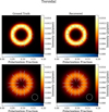 |
Fig. 3 Same as Fig. 2, but the EVPA are following a toroidal magnetic field configuration. |
| In the text | |
 |
Fig. 4 Same as Fig. 2, but the EVPA are following a radial magnetic field configuration. |
| In the text | |
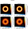 |
Fig. 5 Same as Fig. 2 but the EVPA are following a vertical magnetic field configuration. |
| In the text | |
|
Fig. 6 Cluster of images obtained with MOEA/D for a simulated polarimetric Sgr A* model using EHT+ngEHT array configuration at 230 GHz. |
| In the text | |
|
Fig. A.1 D-terms comparison between the ground truth simulated and that recovered by MOEA/D using closure-only of the source showed in Fig. A.2. Different sites are represented by different colors and markers explained in the legend. The dashed blue lines indicates a perfect correlation. The closer the derms to the line the better correlation between the terms. Top row: DR dterms (real and imaginary part from left to right). Bottom row: DL dterms. |
| In the text | |
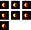 |
Fig. A.2 Same as in Fig. 6, but for this synthetic data set, we applied additional d-term errors. |
| In the text | |
|
Fig. A.3 True movie of the ngEHT Challenge 3 synthetic data (Roelofs et al. 2023). Observation has been divided in 10 keyframe, each of them has been regridded to the MOEA/D resolution, namely, to 10 µas pixels. EVPA are represented as lines and their corresponding polarization fraction appears as color map: the bluer, the stronger m. The intensity of the source is represented by other color map. |
| In the text | |
|
Fig. A.4 Recovered movie of the ngEHT Challenge 3 synthetic data (Roelofs et al. 2023). Each keyframe (which corresponds to exactly the same keyframes depicted in A.3) has been regridded to the MOEA/D resolution, namely, to 10 µas pixels. |
| In the text | |
|
Fig. A.5 Single keyframe at UTC 11.3 recovered from the third ngEHT analysis challenge, with the ground truth image on the left and the recovered keyframe in the right panel. The keyframe has been regridded to the MOEA/D resolution: 10 µas pixels. |
| In the text | |
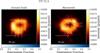 |
Fig. A.6 Same as Fig. A.5, but at UTC 11.5. |
| In the text | |
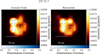 |
Fig. A.7 Same as Fig. A.7, but at UTC 11.7. |
| In the text | |
|
Fig. A.8 Comparison reconstructions of Johnson et al. (2017) method and MOEA/D for the different uυ-coverages of each keyframe. The color scale is linear and is consistent among different times, but is scaled separately for each case, based on the maximum brightness over all frames. The normal cross-corrleation (nxcorr) value between the recovered and the convolved model can be found in the bottom corner of the reconstructed images. A frame-wise comparison can be found in Mus (2023). |
| In the text | |
|
Fig. A.9 Phase diagrams as presented in Mus & Martí-Vidal (2024). Horizontal axis represent the time (frames) and vertical axis the angle. Keyframes are linearly interpolated in every integration time. Left panel: Model corresponding to the dynamical movie. Right panel: Recovered movie. We can see how MMOEA/D is able to recover the hotpsot movement (brightest lines). |
| In the text | |
|
Fig. A.10 Similar to Fig. A.9 but only giving the peak brightness angle versus time (top). The lack line is the ground truth and blue line the recovered solution. In the bottom panel, nxcorr is given for every frame. |
| In the text | |
|
Fig. A.11 Amplitude, β2, of the model (black dots), of the reconstruction (green dots), and the complex norm of their difference (blue dashed lines). |
| In the text | |
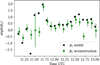 |
Fig. A.12 As in Fig. A.11, but the phases of β2 are represented. |
| In the text | |
|
Fig. A.13 The net polarization as a function of time. |
| In the text | |
|
Fig. B.1 Pareto fronts for the first (top left), second (top right) and third (bottom left) keyframe for the MJ2017 data. Bottom right panel shows the µngMEM dependence with respect to the data fidelity term. |
| In the text | |
Current usage metrics show cumulative count of Article Views (full-text article views including HTML views, PDF and ePub downloads, according to the available data) and Abstracts Views on Vision4Press platform.
Data correspond to usage on the plateform after 2015. The current usage metrics is available 48-96 hours after online publication and is updated daily on week days.
Initial download of the metrics may take a while.