| Issue |
A&A
Volume 683, March 2024
|
|
|---|---|---|
| Article Number | A13 | |
| Number of page(s) | 15 | |
| Section | Interstellar and circumstellar matter | |
| DOI | https://doi.org/10.1051/0004-6361/202347913 | |
| Published online | 28 February 2024 | |
Influence of protostellar outflows on star and protoplanetary disk formation in a massive star-forming clump
1
Université Paris-Saclay, Université Paris-Cité, CEA, CNRS, AIM, 91191 Gif-sur-Yvette, France
e-mail: This email address is being protected from spambots. You need JavaScript enabled to view it.
2
Université Paris-Cité, Université Paris-Saclay, CEA, CNRS, AIM, 91191 Gif-sur-Yvette, France
3
INAF – Istituto di Astrofisica e Planetologia Spaziali (INAF-IAPS), Via Fosso del Cavaliere 100, 00133 Roma, Italy
4
Universität Heidelberg, Zentrum für Astronomie, Institut für theoretische Astrophysik, Albert-Ueberle-Str. 2, 69120 Heidelberg, Germany
5
Universität Heidelberg, Interdisziplinäres Zentrum für Wissenschaftliches Rechnen, Im Neuenheimer Feld 205, 69120 Heidelberg, Germany
6
Dipartimento di Fisica e Astronomia “Augusto Righi”, Viale Berti Pichat 6/2, Bologna, Italy
7
INAF – Osservatorio Astrofisico di Arcetri, Largo E. Fermi 5, 50125 Firenze, Italy
Received:
8
September
2023
Accepted:
5
December
2023
Abstract
Context. Due to the presence of magnetic fields, protostellar jets or outflows are a natural consequence of accretion onto protostars. They are expected to play an important role in star and protoplanetary disk formation.
Aims. We aim to determine the influence of outflows on star and protoplanetary disk formation in star-forming clumps.
Methods. Using RAMSES, we performed the first magnetohydrodynamics calculation of massive star-forming clumps with ambipolar diffusion; radiative transfer, including the radiative feedback of protostars; and protostellar outflows while systematically resolving the disk scales. We compared this simulation to a model without outflows.
Results. We found that protostellar outflows have a significant impact on both star and disk formation. They provide a significant amount of additional kinetic energy to the clump, with typical velocities of around a few 10 km s−1; impact the clump and disk temperatures; reduce the accretion rate onto the protostars; and enhance fragmentation in the filaments. We found that they promote a more numerous stellar population. They do not impact the low-mass end of the IMF much, which is probably controlled by the mass of the first Larson core; however, they have an influence on its peak and high-mass end.
Conclusions. Protostellar outflows appear to have a significant influence on both star and disk formation and should therefore be included in realistic simulations of star-forming environments.
Key words: hydrodynamics / magnetohydrodynamics (MHD) / turbulence / protoplanetary disks / stars: formation / stars: jets
© The Authors 2024
 Open Access article, published by EDP Sciences, under the terms of the Creative Commons Attribution License (https://creativecommons.org/licenses/by/4.0), which permits unrestricted use, distribution, and reproduction in any medium, provided the original work is properly cited.
This article is published in open access under the Subscribe to Open model. This email address is being protected from spambots. You need JavaScript enabled to view it. to support open access publication.
1 Introduction
Fast ejection of matter is an expected consequence of magnetized flows through magneto-centrifugal launching mechanisms (Blandford & Payne 1982). These so-called jets or outflows are ubiquitous around protostars. The typical velocities of molecular outflows have been observed to be at a few 10 km s−1, while strongly collimated jets can reach even higher velocities, >100 km s−1 (see the reviews by Frank et al. 2014; Pascucci et al. 2023).
In numerical models, outflows are either launched self-consistently or through sub-grid modeling. The latter method is often used to investigate their large-scale influence in isolated collapses (e.g., Offner & Chaban 2017; Rohde et al. 2022) as well as on star-forming cloud models (e.g., Carroll et al. 2009; Wang et al. 2010; Cunningham et al. 2011; Federrath et al. 2014; Murray et al. 2018; Li et al. 2018; Guszejnov et al. 2021; Verliat et al. 2022; Grudić et al. 2022; Mathew et al. 2023). Generally, outflows have been shown to play an important role in star formation, reducing the star-formation rate and perhaps even controlling the peak of the stellar initial mass function (IMF) by setting a mass scale, as proposed by several studies (Li et al. 2018; Guszejnov et al. 2021; Mathew et al. 2023).
At small scales, protoplanetary disks are expected to form through angular momentum conservation. As the progenitors of planets, they are very important astrophysical objects. Over the past few years, significant efforts to resolve disk populations in massive star-forming clumps have been made by the astronomical community. Such numerically costly calculations were first performed by Bate (2018), who included a treatment of the radiative transfer but without accounting for magnetic fields. Elsender & Bate (2021) later investigated the impact of the metallicity on disk formation with similar models. The role of magnetic fields in disk formation was investigated first by Kuffmeier et al. (2017, 2019) for such simulations. They, however, did not systematically resolve the disk scales but rather zoomed-in on a few specific disks. Disk populations were then explored while accounting for non-ideal MHD effects for low-mass (Wurster et al. 2019) and high-mass (Lebreuilly et al. 2021) star-forming clumps. In Lebreuilly et al. (2021), we showed that magnetic fields play an important role in regulating the typical disk size in clumps as well as the number of stars in a cloud. In Hennebelle et al. (2022), we showed that they were also affecting the shape of the IMF, as strongly magnetized clouds produce a stellar population with a more top-heavy IMF than weakly magnetized ones. So far, none of these models have accounted for protostellar outflows.
In this paper, we present the first star-forming clump simulation that includes ambipolar diffusion, radiative transfer (including the feedback from a star’s internal and accretion luminosity), and a sub-grid modeling of protostellar outflows as implemented by Verliat et al. (2022) while systematically resolving the disks up to ~1 au. We aim to study the impact of outflows on both star and disk formation and on the clump evolution. We thus compare our simulation with a model without outflows.
The article is organized as follows. In Sect. 2, we present our methods, which are largely similar those of our previous works (Lebreuilly et al. 202l). In Sect. 3, we discuss our results, describing the impact of protostellar outflows. In particular, we present their impact on the density and velocity structure of a cloud, on the population of protoplanetary disks, and on star formation. Finally, we present our conclusions in Sect. 4.
2 Methods
In this section, we describe the essential aspects of our methods. We point out that, outflows and resolution aside, the calculations presented here are the same as the NMHD run from Lebreuilly et al. (2021).
2.1 Setup
We computed our models using the RAMSES code (Teyssier 2002; Fromang et al. 2006) and its extension to radiation hydrodynamics (Commerçon et al. 2011), non-ideal MHD (Masson et al. 2012), and sink particles (Bleuler & Teyssier 2014). As in Lebreuilly et al. (2021), we initially considered a 1000 M⊙ clump with a uniform density. The corresponding size R0 of the clumps of temperature T0 = 10 K were initialized according to the thermal-to-gravitational energy ratio α = 0.08 as
 (1)
(1)
where we define the gravitational constant 𝒢, the Boltzmann constant kB, the hydrogen atom mass mH, and the mean molecular weight µg = 2.31. This leads to an initial density of ~3 × 10⁻¹⁹g cm−3. In addition, we initialized the velocity with supersonic turbulent fluctuations at Mach 𝓜 = 7 with a power spectrum of k−11/3.
Finally, we assumed an initially uniform vertical magnetic field fixed according to the mass-to-flux over critical-mass-to-flux ratio µ = 10 as
 (2)
(2)
the critical mass-to-flux ratio being  (Mouschovias & Spitzer 1976). This corresponds to a magnetic field strength of 9.4 × 10⁻⁵ G. We point out that we only consider the impact of ambipolar diffusion here; the resistivity was computed using the table from Marchand et al. (2016). The Ohmic dissipation is expected to play a role at densities higher than those we resolve here. In addition, the Hall effect could play a significant role, but accounting for it unfortunately remains too challenging in such simulations.
To accurately follow the gas dynamics up to the scales of protoplanetary disks, we took advantage of the adaptive mesh refinement (AMR) grid (Berger & Oliger 1984) of RAMSES. In this work, we refined the grid according to a modified Jeans length defined as
 (3)
(3)
This modification in the refinement criterion is similar to Lebreuilly et al. (2021) and was done to ensure that the hot disk component is always refined up to the maximal resolution. Here, we imposed having ten points per modified Jeans length up to a resolution of 1.2 au. This is enough to avoid artificial fragmentation of the cloud according to the criterion of Truelove et al. (1997) while being computationally affordable. We point out that our coarser cells are ~2460 au.
2.2 Implementation of the protostellar outflows
We used sink particles to mimic protostars. We refer the reader to Bleuler & Teyssier (2014) for more extensive details of their implementation. As in Lebreuilly et al. (2021), we considered that a fraction of the accretion luminosity facc is radiated away by protostars under the form of an accretion luminosity written as
 (4)
(4)
As in Lebreuilly et al. (2021), we considered the case facc = 0.1. The stellar radius, R★, was computed using the evolutionary tracks of Kuiper & Yorke (2013). As explained by Commerçon et al. (2022), these pre-main sequence (PMS) tracks were computed using the STELLAR radiation code. In our case, we used a tabulated version of these tracks as a function of the mass accretion rate (their different models) onto the sink and the stellar mass. The initial object assumed by these models is 0.05 M⊙ and has a radius of 0.56R⊙ and a luminosity of 2.2 × 10⁻² L⊙.
In the case of our model with protostellar outflows, we employed a sub-grid modeling previously implemented in RAMSES by Verliat et al. (2022). We recall the general principle of the methods here. As in Lebreuilly et al. (2021), the sinks of our model accrete, at each time step, a fraction of the mass above the density threshold nthre = 1013 cm−3. In the case of our outflows model, a fraction of the mass that should be accreted, hereafter facc,outflows, is rather ejected in a bipolar cone of opening angle θoutflows at a fraction facc,outflows of the escape velocity. The direction of this cone is then given by the angular momentum direction of the sinks. We refer the reader to Appendix A.1 of Verliat et al. (2022) for the technical details about the implementation of the outflows methods in RAMSES. In this work, we investigated a single configuration for the outflows (i.e., facc,outflows = 1/3, fesc,outflows = 1/3 and θoutflows = 20°). We emphasize that this parameter choice is based on observational evidence, as explained, again, in of Verliat et al. (2022). As they argue, both theoretical (e.g., Blandford & Payne 1982; Pudritz & Norman 1986) and observational (Hartmann & Calvet 1995; Cabrit et al. 2007) studies indicate that facc,outflows is between 0.1 and 0.4, while fesc,outflows should range between 0.25 and 0.5. In addition, and as explained by Guszejnov et al. (2021), the effect of outflows (their lever arm) is actually controlled by the product of these two parameters, and a value of 0.3 for both parameters puts the product in the middle of the range constrained by observations (Cunningham et al. 2011).
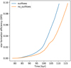 |
Fig. 1 SFE as a function of time for both models. The outflows significantly slow down star formation near the cluster. |
3 Results
Here, we introduce our two models: NO_OUTFLOWS and OUTFLOWS. Both were computed according to the methods described in Appendix 2. For OUTFLOWS, we included the proto-stellar outflows as described in Sect. 2.2, while NO_OUTFLOWS was computed without outflows. We display the evolution of our models in terms of star-formation efficiency (SFE), which is the ratio of the mass of formed sink over the initial clump mass. Our models are presented up to SFE=0.1, which corresponds to the accretion of 100 M⊙ within sink particles. As a supplementary material, we show the evolution of the SFE against time for both models in Fig. 1. One can clearly see that the outflows slow down star formation, as they provide an additional source of mechanical support against collapse and increase the time to reach a given SFE by about 15%–20%.
3.1 Impact on the large-scale structures
In this section, we present a global description of the OUTFLOWS model and compare it with a NO_OUTFLOWS run. In Fig. 2, we show the column density and the mass averaged velocity norm integrated along the z direction, respectively, for NO_OUTFLOWS (top) and OUTFLOWS (bottom). The images are displayed at SFE=0.1 and centered around sink 1, located near the collapse center. From left to right, we show these maps for decreasing scales.
For both runs, a network of star-forming filaments is clearly noticeable. This is an expected consequence of gravo-turbulent motions. As already reported in Lebreuilly et al. (2021), a main star cluster, observed for both models, forms at the vicinity of sink 1. Noticeably, the density maps of the two models are very similar, particularly at large scales (>0.1 pc). Similar behavior was also noted in the previous studies of Krumholz et al. (2011), Guszejnov et al. (2021) and Verliat et al. (2022). We point out that significant differences appear when looking at rather small scales (<0.1 pc), which also in line with the aforementioned studies. These differences between the two models are more striking near the main star cluster. One can clearly see that more stars are able to form in this location in the case of OUTFLOWS; this effect is described more in detail in Sect. 3.3. When focusing on the velocity maps, we noticed that they are also affected by the outflows. In particular, we observed individual outflows quite distinctively. By the end of the simulation, the affected region reached a scale of ~0.1 pc. This is consistent with a propagation at roughly a few 10 km s−1. This is also in agreement with molecular outflow observations (see e.g., Maury et al. 2009; Cunningham et al. 2018) as well as previous numerical works (Federrath et al. 2014; Li et al. 2018; Guszejnov et al. 2021; Verliat et al. 2022).
In Fig. 3, we show the evolution of the total kinetic (plain lines) and magnetic (dotted lines) energies for the two models against the SFE in a radius of 0.1 pc around sink 1, which we call the main cluster (top), as well as in the full clump (middle) and for various velocity thresholds in the cluster (bottom). For both models, the kinetic energy in the main cluster increases over SFE and lies between a ~1046 and ~1047 erg (while the total kinetic energy ranges between ~5 × 1046 and ~1.8 × 1047 erg). As was also reported by previous studies (see Nakamura & Li 2007; Carroll et al. 2009, and the other numerical works cited above), outflows clearly provide additional support for the cloud but operate mostly at small scales. Indeed, a significant amount of kinetic energy is added to the clump by the outflows. Near the end of the calculation, the kinetic energy around the main cluster was about two to three (depending on time and scale) times larger when outflows were included. In total, outflows bring about 50– 70% more kinetic energy to the full clump. Given that in total about 40 M⊙ was ejected by the outflows, the additional kinetic energy of ~5 × 1046 erg brought by the outflows to the full clump is consistent with a bulk velocity of a few 10 km s−1. Notably, the extra kinetic energy brought by the outflows is mostly under the form of a high >10 km s−1 velocity component rather than under the form of turbulence. This can be seen in the bottom panel of Fig. 3, where we show the kinetic energy of the cluster with various velocity thresholds. The kinetic energies for υ < 5 km s−1 and v < 10 km s−1 are indeed much closer to each other in the two models. Quite interestingly, the magnetic energy of OUTFLOWS also increases with respect to NO_OUTFLOWS, as outflows not only provide additional kinetic energy but are also able to increase the magnetic support.
Outflows clearly enhance the fragmentation at the filament scale. This can be seen in Fig. 2 (and Fig. A.1, which displays the same information as Fig. 2 but for SFE=0.05). Quite clearly, the OUTFLOWS clump is more fragmented and disturbed than the NO_OUTFLOWS clump at both SFE=0.05 and 0.1. This effect is particularly visible at scales below 0.05 pc (right panels of the figure) near the main star cluster or in filaments at SFE=0.05.
Figure 4 demonstrates that outflows indeed support fragmentation in the filaments. With this figure, we show the inverse cumulative distribution function (CDF) of density in the dense gas at SFE = 0.05 and SFE=0.1 for the two models. We have excluded the cluster from the CDF, as star formation occurs mostly in the filaments. Here, one can clearly see that a significantly larger fraction of the gas is dense (filament, cores, and disks) when the outflows are accounted for. In Fig. 5, we also observed that effect quite clearly. In these maps, we show the evolution of the column density for one filament located right above the main cluster at three different SFEs (0.05, 0.08, and 0.1, from left to right) both without (top) and with (bottom) outflows. One can clearly see that the filaments are more fragmented in OUTFLOWS than in NO_OUTFLOWS.
In the lower panels of Fig. 5, we show the temperature of the filaments (integrated along the line of sight) at three evolutionary stages with and without outflows. Quite distinctively, not only the background temperature but more importantly the filament temperature is lowered by the presence of outflows. Without outflows, the filament temperature increases by up to 40–50% at SFE=0.08. As we show in Sect. 3.2, this is a consequence of having less stellar feedback, which results from the reduction of the accretion rates by outflows. Reduced stellar feedback has been shown to favor fragmentation by Hennebelle et al. (2020, 2022). In fact, in the top panels of Fig. 5, we even observed a thickening of the arc-shaped filament (as it gets hotter through the effect of stellar feedback) and a suppression of fragmentation over time, whereas the filaments in the bottom panels (i.e., with outflows) remain thinner and more fragmented. We point out that the kinetic energy added by the outflows might also be playing a role in the increased fragmentation. Indeed, an enhanced fragmentation was observed by Wang et al. (2010) with isothermal calculations. As such, the excess of fragmentation could only come from the modification of the cloud dynamics in their case.
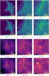 |
Fig. 2 Evolution of the star-forming clump. Top 6 maps: (x−y) column density maps of the two models integrated along the z direction at SFE=0.1. The top map shows the model without protostellar outflows. The bottom map shows the model with protostellar outflows. From left to right: we zoom toward sink 1, that is, near the center of the collapse. The outflows have a visible impact on the column density structures at scales below 0.1 pc. Clearly, more stars form in the presence of the outflows. Bottom 6 maps: same but for the mass weighted norm of the velocity. The outflows significantly modify the velocity field at scales smaller than 0.1 pc. |
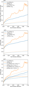 |
Fig. 3 Evolution of the energy for the two models. The top and middle plots show the kinetic (plain lines) and magnetic (dotted lines) energies as a function of SFE for the two models in a sphere of 0.1 pc surrounding the main cluster (top) and in the full clump (middle). As can be seen, outflows increase the overall support of the cloud, as both the kinetic and magnetic energy are larger in their presence. The bottom plots show the kinetic energy in the cluster with various velocity thresholds. We observed that outflows essentially add kinetic energy in a fast v > 10 km s−1 component. |
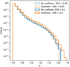 |
Fig. 4 Inverse cumulative distribution function of ρ for the dense gas (for r > 10−15g cm−3) outside the main star cluster, that is, for r > 0.1 pc for both models at SFE=0.05 (dotted lines) and SFE=0.1 (plain lines). One can clearly see that the outflows promote fragmentation between SFE=0.05 and SFE=0.1. |
3.2 Impact on the disk population
Next, we focus on the impact of the protostellar outflows on the disk populations. We refer the reader to Lebreuilly et al. (2021) for our method to extract the disk’s internal properties. However, contrary to Lebreuilly et al. (2021), we selected the disk material using only two of the Joos et al. (2012) criterion: n > ndisk = 109 cm−3, with n being the gas number density, and υ ϕ > 2υr, υ ϕ > 2υz, with υr, υz, and υ ϕ being the radial, vertical, and azimuthal velocity components in the frame of the analyzed sink.
We did not include any condition regarding the gas pressure, as this could arbitrarily remove some of the hot component of the inner disk. The choice of ndisk, though typically used in previous works, remains somewhat arbitrary. As such, we discuss it in Appendix C.
Once the disk cells were extracted, the average of any given quantity Q in the disk (e.g., the disk temperature) was calculated as follows:
 (5)
(5)
Here Δxj is the cell size, and the sum is calculated for each disk cell.
We show the evolution of the disk radius (top-left), mass (top-right), and temperature (bottom-left) as well as the accretion rate onto the star (bottom-right) as a function of the SFE for both models (NO_OUTFLOWS in blue and OUTFLOWS in orange) in Fig. 6. The lines represent the distribution median, and the transparent regions represent the area between its first and third quartile. As such, these figures allow for the visualization of the full disk population as a function of the sFE. some typical protostellar disks are displayed in Appendix B for both runs as supplementary material.
We first focus on the disk size and masses presented in Fig. 6. Quite clearly, the outflows do not have a significant influence on the two quantities. In terms of size, the disks are typically quite compact, with a median radii between ~30 and ~60 au, depending on the time. The radii evolution is very similar for both models. They are in agreement with the previous models of Lebreuilly et al. (2021) and the observations of disks around Class 0 protostars (e.g. Maury et al. 2019; Tobin et al. 2020; Sheehan et al. 2022). For both models, the disk masses typically range between a few 0.01 M⊙ and 0.2 M⊙. Again, outflows do not appear to have a significant impact. The measured disk masses agree quite well with those found in the hydrodynamical calculations of Bate (2018) and Elsender & Bate (2021). We point out that, as noted in Lebreuilly et al. (2021), our disk masses are typically greater than the minimum solar mass nebula limit (MSMN; Hayashi 1981),and as such, they have enough material to form solar-like planetary systems. This is consistent with an early planet formation as a solution for the potential mass-budget problem of T-Tauri disks (Manara et al. 2018).
We next focus on the disk temperature that is most affected by the inclusion of outflows. First of all, it is useful to point out that the accretion luminosity is quite clearly controlling the temperature. In Fig. 7, we show the temperature of the disk versus the accretion luminosity (left) as well as versus the sink mass (middle) and the mass accretion rate onto the sink (right). Each marker corresponds to a disk. The disks are all displayed every 1000 yr from their birth to the end of the simulation. The black line represents the correlation  Quite clearly, a very similar correlation can be observed for both models, and the high-temperature part of the plot is not populated for OUTFLOWS, as the outflows prevent an accretion that would be too strong from happening. The decrease of temperature for high-Lacc in the outflows case is a combined effect of lower mass and lower-mass accretion rates. We indeed clearly observed that, for a given mass range, the low temperature quadrant is more populated for the case of OUTFLOWS. We point out that the aforementioned scaling is expected in the flux-limited diffusion (FLD) approximation (see Hennebelle et al. 2022) for a passively irradiated disk. Because the accretion is high at early stages, the disks are generally quite hot, especially in the case of NO_OUTFLOWS. For this model, the median temperature of the disk quickly reaches high values, around 200–300 K. Notably, the typical disk temperature is lower by a factor of approximately two when outflows are included. This is because the accretion rate onto the protostars are significantly reduced when outflows are included. Owing to the relatively weak scaling between the temperature and the accretion luminosity, only an important change in the accretion luminosity would affect the disk temperatures significantly. This is exactly what occurs in our two runs. As can be seen in panel d, when outflows are included, the typical accretion rate decreases by a factor of a few. Consequently, the median accretion luminosity, which scales as
  , is about one order of magnitude lower when including the protostellar outflows, with a median value of ~50 L⊙ for NO_OUTFLOWS and ~5 L⊙ for OUTFLOWS. This can be seen in Fig. 8, which shows the evolution of the accretion luminosity for the two models as a function of SFE. This is perfectly consistent with the factor of two in median disk temperature between the two models according to the scaling previously reported. We point out that the accretion luminosities that we measured are more in line with observations when the outflows are included since young stellar objects (YSOs) seem to have typical luminosities of a few L⊙ (Maury et al. 2011; Dunham & Vorobyov 2012; Fischer et al. 2017). In addition, outflows could be important to regulating the accretion rate and solving the luminosity problem of YSOs, as a complement to episodic accretion (Offner & McKee 2011; Dunham & Vorobyov 2012; Meyer et al. 2022; Elbakyan et al. 2023).
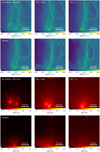 |
Fig. 5 Close-up look at a filament located above the main star cluster at three SFEs (0.05, 0.08, and 0.1) for the two models. The top panels display the column density, and the bottom panels show the temperature integrated along the line of sight. |
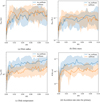 |
Fig. 6 Evolution of the median of the disk radius, the disk mass, the disk temperature, and the mass accretion rate onto the primary as a function of the SFE for the NO_OUTFLOWS (blue) and OUTFLOWS (orange) models. The regions with transparent colors represent the area between the first and third quartile of the distribution. One can clearly see that outflows do not significantly impact the disk size and mass but largely influence their temperature through a reduced accretion rate (and luminosity). |
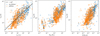 |
Fig. 7 Disk temperature vs. their accretion luminosity (left), the mass of the sink (middle), and the accretion rate onto the sink (right) for both models. All disks are displayed every 1000 yr. The black line denotes the correlation |

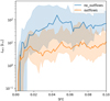 |
Fig. 8 Same as Fig. 6 but for the accretion luminosity. One can clearly see that this quantity is decreased by about an order of magnitude as a consequence of the decreased accretion rate and decreased stellar mass. |
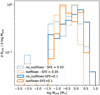 |
Fig. 9 Stellar mass spectrum of the two models at SFE=0.05 (dotted lines) and SFE=0.1 (plain lines). Outflows do not affect the number of low-mass stars (i.e., below a few 0.1 M⊙) but affect the number of more massive stars. In particular, they tend to increase the number of stars with masses around 0.3 M⊙ and reduce the number of the most massive stars. |
3.3 Impact on star formation
Finally, we describe how star formation proceeds in the clump and how the stellar IMF is affected by the inclusion of protostellar outflows. As previously explained, the two models have been integrated up to an SFE of 0.1, which corresponds to t0 + 38.5 kyr for OUTFLOWS and t0 + 32.5 kyr for NO_OUTFLOWS, t0 = 78 kyr being the time of formation of sink 1. Before this time, the two models were identical. Protostellar outflows reduce the time needed to achieve a given SFE by 15–20%. We could also clearly see in Fig. 1 that, at around t = 110 kyr, the SFE is of the order of 0.1 for NO_OUTFLOWS and 0.05 for OUTFLOWS, meaning that the star-formation rate is reduced by roughly a factor of two by the outflows, which is consistent with the accretion rates that we report in this article. Physically, this is not a surprise, as outflows imply that a fraction of the mass above the accretion threshold is ejected rather than accreted. As pointed out earlier, in addition to slowing down accretion, the inclusion of outflows also increases fragmentation, and this allows the clump to form significantly more stars. Indeed, by SFE=0.1, OUTFLOWS has formed 133 sinks, while NO_OUTFLOWS has only formed 84. We point out that for both models, star formation mainly occurs in the dense filaments of the clump. Even the main star cluster originates from filaments, which are later destabilized by the global dynamics of the clump and, in the case of OUTFLOWS, by the outflows.
We show in Fig. 9 the ΓMF of the two clumps at SFE=0.05 (dotted lines) and SFE=0.1 (plain lines). We note that the outflows do not seem to visibly shift the low-mass stars part of the IMF (i.e., the stars with a mass below 0.1 M⊙). Indeed, as we resolved the first Larson core mass, which, as shown by Hennebelle et al. (2019), is a good candidate as a mass scale for the IMF, we were able to probe the transition from an isothermal to an adiabatic equation of state. This stopped the fragmentation in lower-mass objects because at least one first hydrostatic core mass (about 0.03 M⊙) is required at the high densities for the introduction of sink particles.
Outflows, however, affect the shape of the high-mass part of the IMF, or, as argued by Li et al. (2018); Guszejnov et al. (2021); Mathew et al. (2023), its peak. We stress that the differences we observed between the IMFs obtained with and without outflows are significantly lower than what is reported, for instance, in Fig. 6 of Guszejnov et al. (2021). This is likely because in our simulations, the transition from the isothermal to adiabatic regime is resolved. Without outflows, the median stellar mass is about 1 solar mass, and the IMF is quite flat between ~0.2 and ~2 M⊙, in agreement with our previous calculations (Hennebelle et al. 2022). When outflows are included, the IMF is not top heavy anymore, and we observed a more distinctive peak around 0.1–0.3 M⊙. Outflows also appear to play a role in regulating the mass of the most massive stars in cluster Mmax and, more generally, the mass of the stars above ~0.3 M⊙. Here, Mmax ~ 9.4 M⊙ for NO_OUTFLOWS, and it is only 4.1 M⊙ for OUTFLOWS. We believe this could be due to the transition from a thermal and magnetically supported regime to a turbulence and kinetically supported regime, as predicted by the model of Hennebelle et al. (2022).
As shown in their Appendix B, at a given length R, the transition mass between the two regimes scales as
 (6)
(6)
where σ is the RMS velocity dispersion at the cloud scale R0 and cs is the sound speed. At the transition between the regimes, the terms are roughly equal. As such, we have
 (7)
(7)
or
 (8)
(8)
This yields a critical mass Mcrit for the transition between the two regimes, which scales as
 (9)
(9)
Assuming a typical scaling η = 0.5 shows that this critical mass scales quadratically with the temperature, which is a strong dependency. In addition, it scales as the inverse square root of the turbulent velocity dispersion. Reducing the temperature and increasing the turbulent velocity dispersion would result in a shift toward lower masses of the critical mass. As shown before, outflows reduce the clump and filament temperature by up to 40–50% (at SFE=0.08). Indeed, adding them reduces the accretion rate and therefore also affects the stellar feedback by lowering the accretion luminosity and the temperature at filament scales. This reduction would thus shift the critical mass by about a factor of two, which is consistent with what we observed for the two models. Second, this effect could be helped by the considerable amount of kinetic energy brought by the outflows at small scales. Although, strictly speaking, the bulk of the kinetic energy that is added by the outflows does not seem to be in the form of turbulence, it still seems to provide a support against collapse. This is particularly clear in the main star cluster, where outflows quite visibly modify the structures. We also note that as the outflow kinetic energy scales as  , outflows are expected to have a stronger influence around more massive objects. It is not yet clear which of the two effects plays the most important role in shaping the IMF, as both work toward the same direction. Given the scaling of the transition mass demonstrated above, we believe that the temperature effect could be more significant. Future models exploring the impact of the outflow properties, assuming different assumptions for the radiative transfer (facc) and exploring various cloud configurations while still resolving the disk scales, should be dedicated to understanding this effect in more detail and to determining whether outflows systematically have a strong influence. We also emphasize that our ~1 au resolution unfortunately comes with a high numerical cost, and it has therefore prevented us (so far) from producing large statistical samples of sinks or to running a large number of these models.
4 Conclusion
In this article, we have presented the first simulations of massive star-forming clumps that resolve the protoplanetary disk scales while including ambipolar diffusion, radiative transfer with stellar feedback following the radiation from internal and accretion luminosity, and the mechanical momentum input from outflows. In the following list, we summarize our main findings:
- 1.
Protostellar outflows have a clear impact on the velocity structures in clumps at scales smaller than ~0.1 pc and, to a smaller extent, on column density structures. Beyond their propagation scale, their impact is not distinguishable;
- 2.
With or without protostellar outflows, a population of stars and disks is formed in the star-forming clumps. In both cases, we found that disks are born quite compact because of magnetic braking, in agreement with our previous findings (Lebreuilly et al. 2021). In addition, disks are born massive enough to form planets, according to the minimum solar mass nebula criterion. Protostellar outflows do not significantly affect the size and mass of the nascent disks;
- 3.
Outflows reduce the typical accretion luminosity in the cloud by about one order of magnitude and could therefore be a potential solution for the well-known luminosity problem in YSOs as a complement to episodic accretion (Offner & McKee 2011; Dunham & Vorobyov 2012; Meyer et al. 2022; Elbakyan et al. 2023);
- 4.
The typical temperature of protoplanetary disks is lower by a factor of about two when outflows are included as a consequence of the accretion luminosity being lowered;
- 5.
Protostellar outflows affect the stellar population by allowing the formation of more stars. They also affect the stellar spectrum for masses larger than ~0.3 M⊙, allowing it to switch from a rather flat (top-heavy) regime to a shape more consistent with the Galactic IMF. Importantly, the mass of the most massive star is reduced by a factor of approximately two when they are included, as they impact the stellar radiative feedback by reducing the accretion onto the protostars and provide additional kinetic support against collapse. We also found that the low-mass star population is relatively unaffected by the presence of outflows. We believe this is due to this population being controlled by the mass of the first hydrostatic core.
Ubiquitous around YSOs, protostellar outflows appear to play an important role in regulating both star and disk formation by providing an additional form of support as well as by reducing the impact of the accretion luminosity onto protostars. We strongly encourage the undertaking of future work dedicated to exploring the influence of the unconstrained outflow parameters, such as the fraction of ejected material, the outflows launch velocity, and their opening angle, while still resolving the protoplanetary disk scales.
Acknowledgements
We thank the referee for providing a very constructive report that helped us a lot improving our manuscript. This research has received funding from the European Research Council synergy grant ECOGAL (Grant: 855130). We acknowledge PRACE for awarding us access to the JUWELS supercomputer. This work was also granted access to HPC resources of CINES and CCRT under the allocation A0130407023 made by GENCI (Grand Equipement National de Calcul Intensif). M.G. acknowledges the support of the French Agence Nationale de la Recherche (ANR) through the project COSMHIC (ANR-20-CE31-0009).
Appendix A Clump structure at SFE=0.05
As a complement to Fig. 2, we show in this section the column density for SFE=0.05 for both models. The impact of the outflows is already very visible at that stage, especially at scales below 0.1 pc.
Appendix B Protoplanetary disk gallery
In this section, we show the column density and mass weighted velocity integrated along the line of sight of a few typical protoplanetary disks for run NO_OUTFLOWS and OUTFLOWS. The disks are displayed edge-on at SFE=0.1. The impact of the outflows is very clear in the velocity maps but quite invisible in the column density maps (as outflows are mostly composed of low-density material).
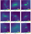 |
Fig. B.1 Column density of a few disks seen edge-on for run NO_OUTFLOWS at SFE=0.1. |
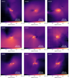 |
Fig. B.3 Same as Fig. B.1 but for the absolute mass weighted norm of the velocity integrated along the line of sight. |
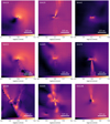 |
Fig. B.4 Same as Fig. B.2 but for the mass weighted norm of the velocity integrated along the line of sight. The outflows have a visible impact on the velocity field. |
Appendix C Influence of the disk selection density criteria
The density criterion of Joos et al. (2012), although useful to separate the disk material from the envelope, remains somewhat arbitrary. Therefore, we varied it by one order of magnitude above and below its reference value of ndisk = 109cm−3 to test its influence on the final estimate of the disk size and mass. We show in Fig.C.1, the evolution of the disk radius and mass as a function of the SFE for the NO_OUTFLOWS and OUTFLOWS models. As can be seen, the mass spectrum is only weakly affected by the change of density threshold, while the disk size is more significantly impacted. In particular, when going from a threshold of 109 cm−3 to a threshold of 108 cm−3, we observed that the disk median radius almost shifts toward 100 au. The difference between 109cm−3 and 1010cm−3 is however much lower (with a shift from ~50 au to about 30–40 au). We not that, by eye, most disks seem to typically have sizes around ~50 au. As such, 109 cm−3 and 1010 cm−3 seem to be a more accurate representation of disks. For continuity with previous studies, we kept the value 109 cm−3. We point out that our choice of disk selection criterion does not matter for the comparison between models, provided that the same method is used to compare the calculations. This could be more problematic when comparing with observed disks. Synthetic observations of the models are needed to really make a one-to-one comparison; a study dedicated to this is currently in preparation.
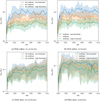 |
Fig. C.1 Disk radius (left) and mass (right) for NO_OUTFLOWS (top) and OUTFLOWS (bottom) as a function of the SFE for three density thresholds for the disk selection. |
References
- Bate, M. R. 2018, MNRAS, 475, 5618 [Google Scholar]
- Berger, M. J., & Oliger, J. 1984, J. Comput. Phys., 53, 484 [NASA ADS] [CrossRef] [Google Scholar]
- Blandford, R. D., & Payne, D. G. 1982, MNRAS, 199, 883 [CrossRef] [Google Scholar]
- Bleuler, A., & Teyssier, R. 2014, MNRAS, 445, 4015 [Google Scholar]
- Cabrit, S., Codella, C., Gueth, F., et al. 2007, A&A, 468, L29 [NASA ADS] [CrossRef] [EDP Sciences] [Google Scholar]
- Carroll, J. J., Frank, A., Blackman, E. G., Cunningham, A. J., & Quillen, A. C. 2009, ApJ, 695, 1376 [NASA ADS] [CrossRef] [Google Scholar]
- Commerçon, B., Teyssier, R., Audit, E., Hennebelle, P., & Chabrier, G. 2011, A&A, 529, A35 [NASA ADS] [CrossRef] [EDP Sciences] [Google Scholar]
- Commerçon, B., Gonzalez, M., Mignon-Risse, R., Hennebelle, P., & Vaytet, N. 2022, A&A, 658, A52 [NASA ADS] [CrossRef] [EDP Sciences] [Google Scholar]
- Cunningham, A. J., Klein, R. I., Krumholz, M. R., & McKee, C. F. 2011, ApJ, 740, 107 [NASA ADS] [CrossRef] [Google Scholar]
- Cunningham, A. J., Krumholz, M. R., McKee, C. F., & Klein, R. I. 2018, MNRAS, 476, 771 [NASA ADS] [CrossRef] [Google Scholar]
- Dunham, M. M., & Vorobyov, E. I. 2012, ApJ, 747, 52 [NASA ADS] [CrossRef] [Google Scholar]
- Elbakyan, V. G., Nayakshin, S., Meyer, D. M. A., & Vorobyov, E. I. 2023, MNRAS, 518, 791 [Google Scholar]
- Elsender, D., & Bate, M. R. 2021, MNRAS, 508, 5279 [NASA ADS] [CrossRef] [Google Scholar]
- Federrath, C., Schrön, M., Banerjee, R., & Klessen, R. S. 2014, ApJ, 790, 128 [NASA ADS] [CrossRef] [Google Scholar]
- Fischer, W. J., Megeath, S. T., Furlan, E., et al. 2017, ApJ, 840, 69 [NASA ADS] [CrossRef] [Google Scholar]
- Frank, A., Ray, T. P., Cabrit, S., et al. 2014, in Protostars and Planets VI, eds. H. Beuther, R. S. Klessen, C. P. Dullemond, & T. Henning (Tucson: University of Arizona Press), 451 [Google Scholar]
- Fromang, S., Hennebelle, P., & Teyssier, R. 2006, A&A, 457, 371 [NASA ADS] [CrossRef] [EDP Sciences] [Google Scholar]
- Grudić, M. Y., Guszejnov, D., Offner, S. S. R., et al. 2022, MNRAS, 512, 216 [CrossRef] [Google Scholar]
- Guszejnov, D., Grudic, M. Y., Hopkins, P. F., Öffner, S. S. R., & Faucher-Giguère, C.-A. 2021, MNRAS, 502, 3646 [NASA ADS] [CrossRef] [Google Scholar]
- Hartmann, L., & Calvet, N. 1995, AJ, 109, 1846 [NASA ADS] [CrossRef] [Google Scholar]
- Hayashi, C. 1981, Progr. Theor. Phys. Suppl., 70, 35 [Google Scholar]
- Hennebelle, P., Lee, Y.-N., & Chabrier, G. 2019, ApJ, 883, 140 [Google Scholar]
- Hennebelle, P., Commerçon, B., Lee, Y.-N., & Chabrier, G. 2020, ApJ, 904, 194 [NASA ADS] [CrossRef] [Google Scholar]
- Hennebelle, P., Lebreuilly, U., Colman, T., et al. 2022, A&A, 668, A147 [NASA ADS] [CrossRef] [EDP Sciences] [Google Scholar]
- Joos, M., Hennebelle, P., & Ciardi, A. 2012, A&A, 543, A128 [CrossRef] [EDP Sciences] [Google Scholar]
- Krumholz, M. R., Klein, R. I., & McKee, C. F. 2011, ApJ, 740, 74 [NASA ADS] [CrossRef] [Google Scholar]
- Kuffmeier, M., Haugbølle, T., & Nordlund, Â. 2017, ApJ, 846, 7 [NASA ADS] [CrossRef] [Google Scholar]
- Kuffmeier, M., Calcutt, H., & Kristensen, L. E. 2019, A&A, 628, A112 [NASA ADS] [CrossRef] [EDP Sciences] [Google Scholar]
- Kuiper, R., & Yorke, H. W. 2013, ApJ, 772, 61 [Google Scholar]
- Lebreuilly, U., Hennebelle, P., Colman, T., et al. 2021, ApJ, 917, L10 [NASA ADS] [CrossRef] [Google Scholar]
- Li, P. S., Klein, R. I., & McKee, C. F. 2018, MNRAS, 473, 4220 [NASA ADS] [CrossRef] [Google Scholar]
- Manara, C. F., Morbidelli, A., & Guillot, T. 2018, A&A, 618, A3 [NASA ADS] [CrossRef] [EDP Sciences] [Google Scholar]
- Marchand, P., Masson, J., Chabrier, G., et al. 2016, A&A, 592, A18 [NASA ADS] [CrossRef] [EDP Sciences] [Google Scholar]
- Masson, J., Teyssier, R., Mulet-Marquis, C., Hennebelle, P., & Chabrier, G. 2012, ApJS, 201, 24 [Google Scholar]
- Mathew, S. S., Federrath, C., & Seta, A. 2023, MNRAS, 518, 5190 [Google Scholar]
- Maury, A. J., André, P., & Li, Z. Y. 2009, A&A, 499, 175 [NASA ADS] [CrossRef] [EDP Sciences] [Google Scholar]
- Maury, A. J., André, P., Men’shchikov, A., Könyves, V., & Bontemps, S. 2011, A&A, 535, A77 [NASA ADS] [CrossRef] [EDP Sciences] [Google Scholar]
- Maury, A. J., André, P., Testi, L., et al. 2019, A&A, 621, A76 [NASA ADS] [CrossRef] [EDP Sciences] [Google Scholar]
- Meyer, D. M. A., Vorobyov, E. I., Elbakyan, V. G., et al. 2022, MNRAS, 517, 4795 [NASA ADS] [CrossRef] [Google Scholar]
- Mouschovias, T. C., & Spitzer, L., Jr 1976, ApJ, 210, 326 [NASA ADS] [CrossRef] [Google Scholar]
- Murray, D., Goyal, S., & Chang, P. 2018, MNRAS, 475, 1023 [NASA ADS] [CrossRef] [Google Scholar]
- Nakamura, F., & Li, Z.-Y. 2007, ApJ, 662, 395 [NASA ADS] [CrossRef] [Google Scholar]
- Offner, S. S. R., & Chaban, J. 2017, ApJ, 847, 104 [NASA ADS] [CrossRef] [Google Scholar]
- Offner, S. S. R., & McKee, C. F. 2011, ApJ, 736, 53 [NASA ADS] [CrossRef] [Google Scholar]
- Pascucci, I., Cabrit, S., Edwards, S., et al. 2023, ASP Conf. Ser., 534, 567 [NASA ADS] [Google Scholar]
- Pudritz, R. E., & Norman, C. A. 1986, ApJ, 301, 571 [NASA ADS] [CrossRef] [Google Scholar]
- Rohde, P. F., Walch, S., Seifried, D., Whitworth, A. P., & Clarke, S. D. 2022, MNRAS, 510, 2552 [NASA ADS] [CrossRef] [Google Scholar]
- Sheehan, P. D., Tobin, J. J., Looney, L. W., & Megeath, S. T. 2022, ApJ, 929, 76 [NASA ADS] [CrossRef] [Google Scholar]
- Teyssier, R. 2002, A&A, 385, 337 [CrossRef] [EDP Sciences] [Google Scholar]
- Tobin, J. J., Sheehan, P. D., Megeath, S. T., et al. 2020, ApJ, 890, 130 [CrossRef] [Google Scholar]
- Truelove, J. K., Klein, R. I., McKee, C. F., et al. 1997, ApJ, 489, L179 [CrossRef] [Google Scholar]
- Verliat, A., Hennebelle, P., Gonzalez, M., Lee, Y.-N., & Geen, S. 2022, A&A, 663, A6 [NASA ADS] [CrossRef] [EDP Sciences] [Google Scholar]
- Wang, P., Li, Z.-Y., Abel, T., & Nakamura, F. 2010, ApJ, 709, 27 [NASA ADS] [CrossRef] [Google Scholar]
- Wurster, J., Bate, M. R., & Price, D. J. 2019, MNRAS, 489, 1719 [NASA ADS] [CrossRef] [Google Scholar]
All Figures
|
Fig. 1 SFE as a function of time for both models. The outflows significantly slow down star formation near the cluster. |
| In the text | |
|
Fig. 2 Evolution of the star-forming clump. Top 6 maps: (x−y) column density maps of the two models integrated along the z direction at SFE=0.1. The top map shows the model without protostellar outflows. The bottom map shows the model with protostellar outflows. From left to right: we zoom toward sink 1, that is, near the center of the collapse. The outflows have a visible impact on the column density structures at scales below 0.1 pc. Clearly, more stars form in the presence of the outflows. Bottom 6 maps: same but for the mass weighted norm of the velocity. The outflows significantly modify the velocity field at scales smaller than 0.1 pc. |
| In the text | |
|
Fig. 3 Evolution of the energy for the two models. The top and middle plots show the kinetic (plain lines) and magnetic (dotted lines) energies as a function of SFE for the two models in a sphere of 0.1 pc surrounding the main cluster (top) and in the full clump (middle). As can be seen, outflows increase the overall support of the cloud, as both the kinetic and magnetic energy are larger in their presence. The bottom plots show the kinetic energy in the cluster with various velocity thresholds. We observed that outflows essentially add kinetic energy in a fast v > 10 km s−1 component. |
| In the text | |
|
Fig. 4 Inverse cumulative distribution function of ρ for the dense gas (for r > 10−15g cm−3) outside the main star cluster, that is, for r > 0.1 pc for both models at SFE=0.05 (dotted lines) and SFE=0.1 (plain lines). One can clearly see that the outflows promote fragmentation between SFE=0.05 and SFE=0.1. |
| In the text | |
|
Fig. 5 Close-up look at a filament located above the main star cluster at three SFEs (0.05, 0.08, and 0.1) for the two models. The top panels display the column density, and the bottom panels show the temperature integrated along the line of sight. |
| In the text | |
|
Fig. 6 Evolution of the median of the disk radius, the disk mass, the disk temperature, and the mass accretion rate onto the primary as a function of the SFE for the NO_OUTFLOWS (blue) and OUTFLOWS (orange) models. The regions with transparent colors represent the area between the first and third quartile of the distribution. One can clearly see that outflows do not significantly impact the disk size and mass but largely influence their temperature through a reduced accretion rate (and luminosity). |
| In the text | |
|
Fig. 7 Disk temperature vs. their accretion luminosity (left), the mass of the sink (middle), and the accretion rate onto the sink (right) for both models. All disks are displayed every 1000 yr. The black line denotes the correlation |
| In the text | |
|
Fig. 8 Same as Fig. 6 but for the accretion luminosity. One can clearly see that this quantity is decreased by about an order of magnitude as a consequence of the decreased accretion rate and decreased stellar mass. |
| In the text | |
|
Fig. 9 Stellar mass spectrum of the two models at SFE=0.05 (dotted lines) and SFE=0.1 (plain lines). Outflows do not affect the number of low-mass stars (i.e., below a few 0.1 M⊙) but affect the number of more massive stars. In particular, they tend to increase the number of stars with masses around 0.3 M⊙ and reduce the number of the most massive stars. |
| In the text | |
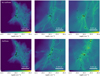 |
Fig. A.1 Same as Fig. 2 but for SFE=0.05. |
| In the text | |
|
Fig. B.1 Column density of a few disks seen edge-on for run NO_OUTFLOWS at SFE=0.1. |
| In the text | |
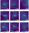 |
Fig. B.2 Same as Fig. B.2 but for OUTFLOWS. |
| In the text | |
|
Fig. B.3 Same as Fig. B.1 but for the absolute mass weighted norm of the velocity integrated along the line of sight. |
| In the text | |
|
Fig. B.4 Same as Fig. B.2 but for the mass weighted norm of the velocity integrated along the line of sight. The outflows have a visible impact on the velocity field. |
| In the text | |
|
Fig. C.1 Disk radius (left) and mass (right) for NO_OUTFLOWS (top) and OUTFLOWS (bottom) as a function of the SFE for three density thresholds for the disk selection. |
| In the text | |
Current usage metrics show cumulative count of Article Views (full-text article views including HTML views, PDF and ePub downloads, according to the available data) and Abstracts Views on Vision4Press platform.
Data correspond to usage on the plateform after 2015. The current usage metrics is available 48-96 hours after online publication and is updated daily on week days.
Initial download of the metrics may take a while.