| Issue |
A&A
Volume 685, May 2024
|
|
|---|---|---|
| Article Number | A91 | |
| Number of page(s) | 16 | |
| Section | Atomic, molecular, and nuclear data | |
| DOI | https://doi.org/10.1051/0004-6361/202347723 | |
| Published online | 14 May 2024 | |
Overview of the contributions from all lanthanide elements to kilonova opacity in the temperature range from 25 000 to 40 000 K★
1
Physique Atomique et Astrophysique, Université de Mons, 7000 Mons, Belgium
e-mail: This email address is being protected from spambots. You need JavaScript enabled to view it.
2
Institut d’Astronomie et d’Astrophysique, Université Libre de Bruxelles, 1050 Brussels, Belgium
3
IPNAS, Université de Liège, 4000 Liège, Belgium
Received:
14
August
2023
Accepted:
12
February
2024
Abstract
Context. It is now well established that the neutron star (NS) merger is at the origin of the production of trans-iron heavy elements in the universe. These elements are therefore present in large quantities in the ejected matter, whose electromagnetic radiation, called kilonova, is characterized by a significant opacity due to the high density of spectral lines belonging to many heavy ions. Among these, the lanthanide ions play an essential role since, with their open 4f subshell, they have a considerable number of transitions that can absorb emitted light. The knowledge of the atomic structure and the radiative parameters of these ions as well as the determination of the corresponding opacities is therefore of paramount importance for the spectral analysis of kilonovae.
Aims. The main goal of the present work is to determine the relative contributions of the different lanthanide elements to the opacity of the emission spectrum of a kilonova in its early phase, that is, a few hours after the NS merger, where the conditions are such that the temperature is between 25 000 and 40 000 K. At these temperatures, the lanthanide ions whose charge states are between V and VII are predominant.
Methods. We used the pseudo-relativistic Hartree–Fock (HFR) method extensively to calculate the relevant atomic data (energy levels, wavelengths, and oscillator strengths) in La-Lu V-VII ions. The corresponding monochromatic opacities were estimated from the expansion formalism.
Results. We calculated the spectroscopic parameters for a total of more than 800 million radiative transitions in all the ions considered. These data were used to estimate the expansion opacities and Planck mean opacities for all the lanthanide elements at early-phase kilonova conditions between 25 000 and 40 000 K, making it possible to deduce the respective contributions of each element as a function of temperature. Atomic calculations were also carried out with the fully relativistic Multiconfiguration Dirac-Hartree-Fock (MCDHF) method in the specific case of the Yb V ion, as the available experimental data had not yet been compared with the theoretical calculations in our previous studies on lanthanide ions.
Key words: atomic data / opacity
The complete atomic data sets used in this paper are available on the Zenodo database at the address https://zenodo.org/records/10635803
© The Authors 2024
 Open Access article, published by EDP Sciences, under the terms of the Creative Commons Attribution License (https://creativecommons.org/licenses/by/4.0), which permits unrestricted use, distribution, and reproduction in any medium, provided the original work is properly cited.
This article is published in open access under the Subscribe to Open model. This email address is being protected from spambots. You need JavaScript enabled to view it. to support open access publication.
1 Introduction
Since the detection of gravitational waves from neutron star (NS) mergers in August 2017, known as the GW170817 event, and its electromagnetic counterpart, called kilonova (Abbott et al. 2017a,b; Kasen et al. 2017), there has been growing interest in studying trans-iron heavy elements. The latter are indeed produced in large quantities by the nucleosynthesis r-process during the NS coalescence and are therefore present in the ejected matter.
As many heavy elements are characterized by complex electronic configurations, giving rise to many energy levels, a large number of radiative transitions absorb the kilonova emitted light and contribute strongly to the opacity affecting the observed spectrum. With their unfilled 4f subshell, the lanthanides (Z = 57–71) are among the main contributors to this opacity. This has motivated many investigations aimed at determining the atomic parameters and opacities of these elements over the past few years. In particular, we mention here the works focused on the first four ionization stages of lanthanides, namely, those related to Nd II–IV (Gaigalas et al. 2019; Flörs et al. 2023); Er III (Gaigalas et al. 2020); Pr–Gd II (Radžiūtė et al. 2020); Tb–Yb II (Radžiūtė et al. 2021); Ce II–IV (Carvajal Gallego et al. 2021); and Ce IV (Rynkun et al. 2022). All lanthanide atoms from I to IV charge stages and the corresponding opacities were also studied by Fontes et al. (2020). All of these works complemented the kilonova simulations initially considered by, for example, Kasen et al. (2013, 2015), Tanaka & Hotokezaka (2013), Barnes & Kasen (2013), Fontes et al. (2015) and Tanaka et al. (2020). Recently, the modeling of the emission spectra of lanthaniderich ejecta following an NS merger at different epochs after the coalescence has also been carried out by different authors, such as Hotokezaka & Nakar (2020), Domoto et al. (2022, 2023), Gillanders et al. (2022, 2024), Tanaka et al. (2023).
With regard to higher ionization degrees of lanthanides, which are of interest for the analysis of early-phase kilonovae, that is, a few hours after the NS merger, some works have been also carried out. Among these are works that we recently published for La V–X (Carvajal Gallego et al. 2022a); Ce V–X (Carvajal Gallego et al. 2022b); Pr–Nd–Pm V–X (Carvajal Gallego et al. 2023a); Sm V–X (Carvajal Gallego et al. 2023b); and Lu V (Maison et al. 2022). To these works must be added the atomic data and opacity calculations performed for three selected lanthanides (Nd, Sm, Eu) and for all the elements from La to Ra, thus including the lanthanides ionized to the states V–XI, by Banerjee et al. (2022, 2023), respectively. In the latter papers, the authors concluded that the lanthanide opacity can be exceptionally high for typical kilonova conditions of T ~ 70000 K at a time t ~ 0.1 day after the NS merger, due to the dense energy levels in highly ionized species, in particular the IX–XI ionization stages that are predominant at such temperatures.
However, using a novel ab initio modeling of the kilonova precursor and kilonova afterglow based on 3D general-relativistic magnetohydrodynamic simulations of NS mergers with nuclear, tabulated, and finite-temperature equations of state, weak interactions, and approximate neutrino transport, Combi & Siegel (2023) found that the predicted opacity boost due to highly ionized lanthanides predicted by Banerjee et al. (2022, 2023) at T ~ 70 000 K was unlikely to affect the early-phase kilonova based on the obtained ejecta structures, as the photosphere in their simulated merger ejecta remained at much lower gas temperatures (typically less than 50000 K) at all times. Therefore, it seems relevant to intensify efforts in the study of atomic processes characterizing atomic systems whose charge stages correspond to temperatures encountered in the kilonova region where the emission of light is significantly affected in practice.
The main goal of the present work is to determine the relative contributions of the different lanthanide elements to the opacity of the emission spectrum of a kilonova in its early phase, that is, a few hours after the NS merger, where the conditions are such that the density is ρ = 10−10 g cm−3 and the temperature is between 25 000 and 40000 K. At these temperatures, the study of the ionization balance reported in our previous papers (Carvajal Gallego et al. 2022a,b, 2023a) showed that the charge states V–VII of lanthanide ions are predominant. We therefore undertook a systematic and detailed study of the atomic structures and the radiative parameters of these ions, namely, La–Lu V–VII, and we deduced the corresponding opacities. To do this, we used extended atomic models based on the pseudo-relativistic Hartree–Fock (HFR) method to obtain the relevant spectroscopic data, whose reliability was already discussed in our previous papers based on detailed comparisons with available experimental and theoretical data. For the ions considered in the present study, this was the case for La V–VII, Ce V–VII, Pr V, Nd V, and Lu V (Carvajal Gallego et al. 2022a,b, 2023a; Maison et al. 2022), of which wavelengths and energy levels deduced from laboratory measurements have been published. The only lanthanide ion for which the available experimental atomic data of Meftah et al. (2013) have not yet been compared with HFR theoretical results is Yb V. In the present work, we carried out this comparison through new calculations performed using the purely relativistic Multiconfiguration Dirac–Hartree–Fock (MCDHF) approach for cross-checking purposes.
2 Atomic data computations
The method used for computing the atomic structures and radiative parameters was the pseudo-relativistic HFR approach developed by Cowan (1981). As discussed in some of our previous works (Flörs et al. 2023; Deprince et al. 2023), this method is particularly well adapted to the determination of opacities because it allows one to obtain atomic data of the same quality for the whole set of states belonging to all the electronic configurations included in a physical model since each of them is optimized by the variational principle, unlike some other commonly used methods, such as those implemented in AUTOSTRUCTURE (Badnell 2011), HULLAC (Bar-Shalom et al. 2001), FAC (Gu 2008), or the General Relativistic Atomic Structure Program (GRASP; Froese Fischer et al. 2016, 2019) codes. Indeed, although the latter theoretical approaches may lead to better results for specific atomic states, the optimization of the calculation is carried out most of the time on a restricted number of configurations so that all the states belonging to the other configurations, namely, those not minimized by the variational principle, cannot be considered as spectroscopic and therefore risk not being of quality equivalent to the optimized states. In this case, all the levels (and therefore the radiative transitions) used to calculate the opacities are not necessarily of the same quality. This is unlike HFR calculations, in which all explicitly included configurations can be considered spectroscopic. In addition, the HFR method used in the present work makes it possible to include a large number of electronic configurations and therefore a large number of atomic states in the calculations, which can be performed in very reasonable computing times.
The ionization stages V–VII of lanthanide elements represent 45 different atomic systems. Among these 45 species, 19 have already been investigated using the HFR method in our previous works, namely, La V–VII (Carvajal Gallego et al. 2022a); Ce V–VII (Carvajal Gallego et al. 2022b); Pr V–VII, Nd V–VII, and Pm V–VII (Carvajal Gallego et al. 2023a); Sm V–VII (Carvajal Gallego et al. 2023b); and Lu V (Maison et al. 2022). For the 26 remaining ions (i.e., Eu V–VII, Gd V–VII, Tb V–VII, Dy V–VII, Ho V–VII, Er V–VII, Tm V–VII, Yb V–VII, Lu VI–VII), new calculations were carried out. For each ion considered in the present study, the configurations introduced in the HFR computations are listed in Table A.1 In the same table, we give the number of radiative transitions involving energy levels below the ionization potential and for which the log ɡf-values were found to be greater than −5 in our calculations. It was indeed shown in previous studies (Carvajal Gallego et al. 2021) that this lower limit on the oscillator strengths allows for the inclusion of the vast majority of transitions contributing to the opacity, and the weaker lines can therefore be neglected. When taking the ionization potentials from the NIST database (Kramida et al. 2023), this gave a number of transitions for a single ion varying from a few tens of thousands to a few tens of millions. The total number of transitions reached about 800 million for the full set of ions considered in our work. We add that in order to better represent the experimental energy structure in the lanthanide ions considered, the Slater integrals (Fk, Gk, Rk) were scaled down by a factor of typically 0.90 in our HFR calculations, as suggested by Cowan (1981). However, we previously showed in Carvajal Gallego et al. (2023a) that the overall properties of opacities were not drastically affected by the choice of this scaling factor and therefore by a small variation in the eigenvector compositions. The final radiative parameters obtained for the large amount of transitions considered in the opacity calculations were changed by at most a few percent. Moreover, we also showed in Deprince et al. (2023) that even if some radial parameters, such as the configuration average energies, are adjusted to correct the calculated energy levels in order to better match experimental values available in the literature, thus slightly modifying the composition mixings of the eigenvectors, the resulting computed opacities are virtually not affected by such a semi-empirical procedure.
From these HFR calculations, we could deduce an initial interesting result, namely, the configuration and the spectroscopic designation of the ground energy level for each ion. This information remained unclear until now, as the data available in the NIST compilation (Kramida et al. 2023) and those published by Kilbane & O’Sullivan (2010) and Banerjee et al. (2023) show frequent disagreement with each other. In Table A.2, we compare the fundamental configurations obtained from our HFR models with those published previously. We noticed that, for most ions, we confirm the recent results of Banerjee et al. (2023), and the only exceptions occur for Pm VII, Eu VII, Gd VII, and Tb VII, for which our calculations give ground configurations of the type 5p64fk, instead of 5p54fk+1 from Banerjee et al. (2023), with k = 1, 3, 4, 5, respectively. It should be noted that for two of these ions (Pm VII and Tb VII), the fundamental configurations deduced from our calculations, namely, 5p64f and 5p64f5, were not included in the theoretical models of Banerjee et al. (2023), while the fundamental configurations obtained by the latter authors were all part of the physical models considered in our work for all ions listed in Table A.2. In addition, it is worth mentioning that the strategy followed by Banerjee et al. (2023) to deduce the ground configurations in lanthanide ions was based on the use of different central potentials in their HULLAC models calculated by changing the electron distribution in 4f and 5p orbitals and optimizing for energy levels belonging to different sets of configurations, while in our HFR calculations, the ground states were systematically obtained with the whole set of configurations included in the physical models, thus allowing all these configurations to influence the determination of the ground state. Furthermore, the 5s, 5p, and 4f orbitals, which are very close to each other in the considered lanthanide ions and therefore play a key role in determining the fundamental configuration, are different for each configuration in our HFR calculation, as already mentioned above. This allowed confidence in the designation of the ground state to be established on the basis of orbitals that are specific to the configuration to which they belong. It is also interesting to note that our results confirm the ground-state configurations published by Kilbane & O’Sullivan (2010) for nearly all ions except Sm VII and Dy VII, whereas the NIST data disagree with our results as well as with those of Kilbane & O’Sullivan (2010) and Banerjee et al. (2023) for many ions. This could be expected in view of the relatively simplified theoretical calculations, most of which are quite old, carried out in different approximations (Carlson et al. 1970; Sugar & Kaufman 1975; Martin et al. 1978; Rodrigues et al. 2004) and used for the designation of the ground states in the NIST compilation for moderately and highly ionized lanthanides. Finally, in Table A.2, we give the LS -coupling designation of the ground level for each ion considered in the present work. This information is provided for the first time.
Among the 45 ions considered in our study, only ten have experimentally measured wavelengths for electric dipole transitions, namely, La V (Epstein & Reader 1976); La VI (Gayasov et al. 1997); La VII (Gayasov et al. 1998); Ce V (Churilov & Joshi 2000); Ce VI (Joshi et al. 2001); Ce VII (Tauheed & Joshi 2008); Pr V (Kaufman & Sugar 1967); Nd V (Meftah et al. 2008; Delghiche et al. 2015); Yb V (Meftah et al. 2013); and Lu V (Kaufman & Sugar 1978; Ryabtsev et al. 2015). With the exception of Yb V, the HFR results have already been compared with all of these experimental data in our previous papers (see Carvajal Gallego et al. 2022a,b, 2023a, Maison et al. 2022). In these papers, it was not only shown that the theoretical wavelengths were in good agreement (within a few percent) with the observed values but also that the (small) differences Δλ = λHFR − λExp were not systematic (i.e. there were as many positive differences as negative). More precisely, by bringing together the results obtained in the articles cited above for the ions La V–VII, Ce V–VII, Pr V, Nd ,V and Lu V, it was found that the average relative difference Δλ/λExp was equal to −0.024 ± 0.037 for a total of 1381 lines. This is shown in Fig. 1, where the values of Δλ/λExp are plotted as a function of λHFR for all the lines for which experimental wavelengths were published in these lanthanide ions. The only ion for which we have not yet made comparisons with existing experimental data in our previous works is Yb V. For the latter, about 1080 lines were observed and identified by Meftah et al. (2013) from the spectrum of ionized ytterbium produced by a sliding spark source recorded on the 10 m high-resolution vacuum ultraviolet normal-incidence spectrograph of the Meudon Observatory. When comparing their experimental wavelengths with those obtained in our HFR calculations, we also found a very good agreement, with the mean deviation Δλ/λExp being found to be equal to 0.018 ± 0.044. The values of Δλ/λExp obtained for all the experimentally observed lines in Yb V are also shown in Fig. 1. We also emphasize that, as the vast majority of the transitions observed in the lanthanide ions considered in the present work were classified by different experimentalists with the LS spectroscopic designations of the lower and higher levels, it was quite simple for us to find all of these transitions in our HFR calculations, which also classify transitions in the same LS -coupling.
With regard to Yb V, we also took the opportunity to compare our HFR oscillator strengths with new results obtained from the purely relativistic MCDHF method (Grant 2007; Froese Fischer et al. 2016) using the latest version of the GRASP, GRASP2018 (Froese Fischer et al. 2019). In these MCDHF calculations, the same strategy as the one considered in our previous works (Carvajal Gallego et al. 2022a,b, 2023a,b) was applied. More precisely, a multireference (MR) set of configurations was chosen to include the 5p64f12, 5p64f116p even-parity and the 5p64f115d, 5p64f116s odd-parity configurations. The 1s–4f orbitals were optimized on all the levels of the 5p64f12 ground configuration using the extended average level (EAL) option (Grant 2007), while the 5d, 6s, and 6p orbitals were optimized on all the levels of the MR configurations using the extended optimal level (EOL) option but keeping all other orbitals fixed. A valence-valence (VV) model was then built by adding single and double (SD) excitations from 6s, 6p, 5d, 4f to all orbitals up to 6s, 6p, 5d, 5f, 5g. For the correlation orbitals 5f and 5g, the EOL option was used where these orbitals were optimized on all the levels of the MR configurations. From the latter model, core-valence (CV) interactions were considered in a relativis-tic configuration interaction (RCI) approach (Grant 2007; Froese Fischer et al. 2019) by adding SD excitations from the 4d core orbital to the MR valence orbitals, namely, 6s, 6p, 5d, and 4f. This gave rise to a total of 1924 269 configuration state functions when considering both parities together. The energy level values obtained in this CV model revealed a good agreement with the experimental data reported in the literature (Meftah et al. 2013), and we found the mean deviation ΔE/EExp (with ΔE = EMCDHF − EExp) to be equal to −0.002 ± 0.040. As a reminder, in fully relativistic MCDHF calculations, the energy level designations are obtained in jj-coupling while, most often, the experimentally observed levels are given in LS -coupling, which is better suited for labeling. Fortunately, the GRASP2018 code includes the jj2lsj routine (Gaigalas et al. 2003, 2017; Jönsson et al. 2023), which makes the task easier and allows, if necessary, transformation of the designations of the calculated levels from jj- to LS -coupling.
In Table A.3, we list the strongest Yb V lines taken from Meftah et al. (2013), that is, those with observed intensities larger than 100. For these lines, we also report the oscillator strengths (log ɡf) obtained in the present work using the HFR and MCDHF methods as well as the values deduced from the transition probabilities (ɡA) calculated by Meftah et al. (2013). From comparisons between these log ɡf-values, shown in Figs. 2 and 3, we found that our HFR results were in good agreement with those obtained with the MCDHF approach results, with the mean deviation between both calculations being found to be equal to 24%. This is quite similar to the agreement of about 30% generally observed between our HFR and MCDHF calculations carried out previously for the ions of lanthanum (Carvajal Gallego et al. 2022a); cerium (Carvajal Gallego et al. 2022b); praseodymium; neodymium (Carvajal Gallego et al. 2023a); and lutetium (Maison et al. 2022), for which detailed comparisons of oscillator strengths computed with both methods can be found in the corresponding papers. However, it appeared that the average difference between our HFR oscillator strengths and the values deduced from Meftah et al. (2013) was about 5%. We note that these comparisons were made by excluding transitions affected by significant cancellation effects in the HFR calculations, that is, for which the cancellation factor (CF), as defined by Cowan (1981), was smaller than 0.1. The transitions concerned are those located at λ = 543.205 (first line), 564.458 (second line), 571.235, 583.541, 589.608, 594.713, 802.074 (second line), and 1709.796 Å. The line at 1577.883 Å was also excluded from the HFR-MCDHF comparison because a very large discrepancy (more than a factor of two) was found between the MCDHF ɡf-values obtained using the Babushkin and Coulomb gauges.
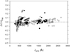 |
Fig. 1 Comparison between the calculated HFR wavelengths and all the available experimentally measured values. The open dots correspond to HFR calculations performed in our previous studies of La V–VII (Carvajal Gallego et al. 2022a); Ce V–VII (Carvajal Gallego et al. 2022b); Pr V, Nd V (Carvajal Gallego et al. 2023a); and Lu V (Maison et al. 2022), while the solid dots correspond to the calculations carried out in the present work for Yb V. |
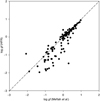 |
Fig. 2 Comparison between the oscillator strengths (log ɡf) obtained in the present work for Yb V transitions using the HFR method and those deduced from the ɡA-values published by Meftah et al. (2013). |
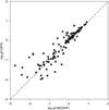 |
Fig. 3 Comparison between the oscillator strengths (log ɡf) obtained in the present work for Yb V transitions using the HFR and the MCDHF methods. |
3 Expansion opacities
In view of the large and consistent set of atomic transitions calculated with the HFR method, whose reliability can be assumed thanks to the few comparisons with other experimental (wavelengths) and theoretical (oscillator strengths) data, as described in Sect. 2, we used the new HFR radiative parameters to compute the opacities corresponding to all lanthanide ions in the charge stages from V to VII, for which the complete atomic data sets are available from the Zenodo database1. To do this, we first determined the expansion opacities using the expression for the absorption coefficient for bound-bound transitions given by
 (1)
(1)
where λ (in Å) is the central wavelength within the region of width, Δλ and λl are the wavelengths of the lines appearing in this range, τl represents the corresponding optical depths, c is the speed of light (in centimeters per second), ρ is the density of the ejected gas (in grams per centimeters cubed), t is the elapsed time since ejection (in seconds), and τl is the optical depth, which can be expressed using the Sobolev formula (Sobolev 1960):
 (2)
(2)
In the latter, e is the elementary charge (in Coulomb), me is the electron mass (in grams), fl is the oscillator strength (dimensionless), and nl is the density of the lower level of the transition (in per cubic centimeter, cm−3), which can be obtained by assuming local thermodynamic equilibrium (LTE) by using the Boltzmann distribution,
 (3)
(3)
where n is the ion density and U(T) is the partition function defined by
 (4)
(4)
where Ei represents all the energy levels belonging to the atomic system with respect to the ground level, ɡi is the corresponding statistical weights (=2Ji + 1), and kB is the Boltzmann constant.
By incorporating in these expressions all the energy levels resulting from the configurations listed in Table A.1 and all the radiative transitions whose number is also given in the same table, we calculated the expansion opacities for the La–Lu V–VII ions corresponding to kilonova conditions where these ionization degrees are dominant, namely, t = 0.1 day; ρ = 10−10 g cm−3, as suggested by Banerjee et al. (2020); and T = 25 000–40 000 K. This temperature range was chosen based on the fact that in our previous studies on La, Ce, Pr, Nd, Pm, and Sm ions (Carvajal Gallego et al. 2022a,b, 2023a,b), the latter systematically showed maximum ionic fractions in their V–VII states for temperatures between 25 000 and 40 000 K.
The expansion opacities are plotted in Figs. 4–7 for the four selected temperatures of T = 25000, 30000, 35000, and 40 000 K, respectively. An initial observation that can be made by examining these figures is that the overall opacity increases with temperature, the latter being almost one order of magnitude higher at 40000 K compared to 25000 K. Indeed, if the maximum opacity varies from about 102 to 10−2 cm2 g−1 at T = 25 000 K for increasing wavelengths between 500 and 10 000 Å, it varies from 103 to 10−1 cm2 g−1 at 40000 K. We also note that the different lanthanide elements do not contribute in the same way to the opacity as a function of temperature. Thus, for example, if one looks at the spectral range beyond 2000 Å, one can notice that the Pr, Sm, and Eu ions have the greatest expansion opacities at T = 25 000 K, whereas the La and Ce ions contribute the most at T = 40000 K.
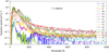 |
Fig. 4 Expansion opacity for lanthanide elements at T = 25 000 K. |
4 Planck mean opacities
The expansion opacities depend on the wavelength of the light being considered. A commonly used wavelength-independent parameter is the Planck mean opacity defined by the expression
 (5)
(5)
where B(λ,T) is the Planck black-body function given by
 (6)
(6)
The Planck mean opacity makes it possible to average the expansion opacities over the entire spectral range as a function of temperature. When calculating κP with the κbb-values obtained in Sect. 3, we deduced the relative contributions of the different lanthanide elements to the kilonova opacity between 25 000 and 40000 K. This is illustrated in Fig. 8, where the Planck mean opacity is plotted as a function of temperature for each of the elements considered in the present work. When looking at this figure, we noticed that the opacity is dominated by Eu, Gd, Tb, Sm, and Dy at 25 000 K, while the predominant elements at 40 000 K are Dy, Tb, Gd, Ho, and Eu. Conversely, some lan-thanide elements, such as Ce, La, Pr, Lu, Pm, Nd, contribute very little to the mean opacity over the entire temperature range, with κP-values one order of magnitude (for T = 40000 K) to two to three orders of magnitude (for T = 25 000 K) lower than those corresponding to the predominant elements cited above. This trend is confirmed in Fig. 9, where the Planck mean opacity is plotted against the atomic number, Z, for all lanthanide elements at T = 25 000 K and T = 40 000 K. These findings are in good overall agreement with the results presented by Banerjee et al. (2023).
However, it is worth noting that if the maximum value of the Planck mean opacity calculated in our work at 25 000 K agrees well with that deduced from Fig. 5 of Banerjee et al. (2023), the maximum opacity obtained by Banerjee et al. (2023) at 40 000 K is approximately three times greater than the result deduced from our study. This could be due not only to the differences in the physical models considered in the respective atomic calculations but also to the differences in the partition function calculations used for the estimation of expansion opacities. In one of our recent papers (Carvajal Gallego et al. 2023c), we indeed showed that the use of realistic partition functions in kilonova opacity calculations leads to a significant deviation from the crude approximation based on a ground-level statistical weight, as commonly assumed in many previous works.
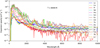 |
Fig. 5 Expansion opacity for lanthanide elements at T = 30 000 K. |
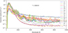 |
Fig. 6 Expansion opacity for lanthanide elements at T = 35 000 K. |
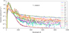 |
Fig. 7 Expansion opacity for lanthanide elements at T = 40 000 K. |
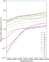 |
Fig. 8 Planck mean opacity for lanthanide elements between 25 000 and 40 000 K. |
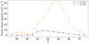 |
Fig. 9 Behavior of the Planck mean opacity with the atomic number, Z, for lanthanide elements at T = 25 000 and 40 000 K. |
5 Conclusions
A new, consistent set of energy levels, wavelengths, and oscillator strengths was obtained for all lanthanide ions between charge states V and VII. To do this, we carried out large-scale calculations using the pseudo-relativistic HFR method, allowing for the determination of radiative parameters for about 800 million transitions in the 45 ions considered in this study. In this work, we complemented the calculations that had already been performed in our previous studies for 19 of these 45 ions, that is, for La V–VII (Carvajal Gallego et al. 2022a); Ce V–VII (Carvajal Gallego et al. 2022b); Pr V–VII, Nd V–VII, Pm V–VII (Carvajal Gallego et al. 2023a); Sm V–VII (Carvajal Gallego et al. 2023b); and Lu V (Maison et al. 2022), with new calculations for the 26 remaining ions, namely, Eu V–VII, Gd V–VII, Tb V–VII, Dy V–VII, Ho V–VII, Er V–VII, Tm V–VII, Yb V–VII, Lu VI–VII. All of these atomic data were then used to estimate the expansion opacities and the Planck mean opacities for early kilonova conditions, that is, a few hours after the NS merger, in the temperature range between 25 000 and 40 000 K. We found that the opacity is dominated by Eu, Gd, Tb, Sm, and Dy at 25 000 K, while the predominant elements at 40 000 K are Dy, Tb, Gd, Ho, and Eu.
As additional results deduced from these calculations, we report the electronic configurations and the spectroscopic designations of the ground states characterizing all the lanthanide ions La–Lu V–VII, which were unclear until now. Moreover, we also provide a detailed comparison between the HFR results and the new fully relativistic MCDHF computations for the specific case of the Yb V ion, as the available experimental atomic parameters had not been compared with the theoretical data in our previous works. For this specific ion, we explicitly report the new atomic results for the first time.
Acknowledgements
H.C.G is holder of a FRIA fellowship while P.P. and P.Q. are, respectively, Research Associate and Research Director of the Belgian Fund for Scientific Research F.R.S.-FNRS. This project has received funding from the FWO and F.R.S.-FNRS under the Excellence of Science (EOS) programme (Grant Nos. O.0228.18 and O.0004.22). Part of the atomic calculations were made with computational resources provided by the Consortium des Équipements de Calcul Intensif (CECI), funded by the F.R.S.-FNRS under Grant No. 2.5020.11 and by the Walloon Region of Belgium.
Appendix A Tables
Configurations included in HFR calculations for lanthanide ions between the V and VII charge stages.
Ground configurations and energy levels of La-Lu V-VII ions.
Calculated oscillator strengths (log gf) for the strongest Yb V lines observed by Meftah et al. (2013).
References
- Abbott, B. P., Abbott, R., Abbott, T. D., et al. 2017a, Phys. Rev. Lett. 119, 161101 [Google Scholar]
- Abbott, B. P., Abbott, R., Abbott, T. D., et al. 2017b, ApJ, 848, L13 [CrossRef] [Google Scholar]
- Badnell, N. R. 2011, Comput. Phys. Commun., 182, 1528 [NASA ADS] [CrossRef] [Google Scholar]
- Banerjee, S., Tanaka, M., Kawaguchi, K., Kato, D., & Gaigalas, G. 2020, ApJ, 901, 29 [NASA ADS] [CrossRef] [Google Scholar]
- Banerjee, S., Tanaka, M., Kato, D., et al. 2022, ApJ, 934, 117 [CrossRef] [Google Scholar]
- Banerjee, S., Tanaka, M., Kato, D., & Gaigalas, G. 2023, ApJ, submitted [arXiv:2304.05810v2] [Google Scholar]
- Barnes, J., & Kasen, D. 2013, ApJ, 775, 18 [NASA ADS] [CrossRef] [Google Scholar]
- Bar-Shalom, A., Klapisch, M., & Oreg, J. 2001, J. Quant. Spectr. Rad. Transf., 71, 169 [NASA ADS] [CrossRef] [Google Scholar]
- Carlson, T. A., Nestor, C. Wasserman, N., & Mcdonell, J. 1970, At. Data Nucl. Data Tables, 2, 63 [NASA ADS] [CrossRef] [Google Scholar]
- Carvajal Gallego, H., Palmeri, P., & Quinet P. 2021, MNRAS, 501, 1440 [Google Scholar]
- Carvajal Gallego, H., Berengut, J. C., Palmeri, P., & Quinet, P. 2022a, MNRAS, 509, 6138 [Google Scholar]
- Carvajal Gallego, H., Berengut, J. C., Palmeri, P., & Quinet, P., 2022b, MNRAS, 513, 2302 [NASA ADS] [CrossRef] [Google Scholar]
- Carvajal Gallego, H., Deprince, J., Berengut, J. C., Palmeri, P., & Quinet, P. 2023a, MNRAS, 518, 332 [Google Scholar]
- Carvajal Gallego, H., Deprince, J., Palmeri, P., & Quinet, P., 2023b, MNRAS, 522, 312 [NASA ADS] [CrossRef] [Google Scholar]
- Carvajal Gallego, H., Deprince, J., Godefroid, M., et al. 2023c, Eur. Phys. J. D, 77, 72 [NASA ADS] [CrossRef] [Google Scholar]
- Churilov, S. S., & Joshi, Y. N. 2000, J. Opt. Soc. Am. B, 17, 2081 [CrossRef] [Google Scholar]
- Combi, L., & Siegel, D. M. 2023, ApJ, 944, 28 [NASA ADS] [CrossRef] [Google Scholar]
- Cowan, R. D. 1981, The Theory of Atomic Structure and Spectra (Berkeley: California University Press) [Google Scholar]
- Delghiche, D., Meftah, A., Wyart, J.-F., et al. 2015, Phys. Scr., 90, 095402 [NASA ADS] [CrossRef] [Google Scholar]
- Deprince, J., Carvajal Gallego, H., Godefroid, M., et al. 2023, Eur. Phys. J. D, 77, 93 [NASA ADS] [CrossRef] [Google Scholar]
- Domoto, N., Tanaka, M., Kato, D., et al. 2022, ApJ, 939, 8 [NASA ADS] [CrossRef] [Google Scholar]
- Domoto, N., Lee, J. J., Tanaka, M., et al. 2023, ApJ, 956, 113 [CrossRef] [Google Scholar]
- Epstein, G. L., & Reader, J. 1976, J. Opt. Soc. Am., 66, 590 [NASA ADS] [CrossRef] [Google Scholar]
- Flörs, A., Silva, R. F., Deprince, J., et al. 2023, MNRAS, 524, 3083 [CrossRef] [Google Scholar]
- Fontes, C. J., Fryer, C. L., Hungerford, A. L., et al. 2015, High Energy Density Phys., 16, 53 [NASA ADS] [CrossRef] [Google Scholar]
- Fontes, C. J., Fryer, C. L., Hungerford, A. L., Wollaeger, R. T., & Korobkin, O. 2020, MNRAS, 493, 4143 [CrossRef] [Google Scholar]
- Froese Fischer, C., Godefroid, M., Brage, T., Jönsson, P., & Gaigalas, G. 2016, J. Phys. B: At. Mol. Opt. Phys., 49, 182004 [CrossRef] [Google Scholar]
- Froese Fischer, C., Gaigalas, G., Jönsson, P., & Bieron, J. 2019, Comput. Phys. Commun. 237, 184 [NASA ADS] [CrossRef] [Google Scholar]
- Gaigalas, G., Zalandauskas, T., & Rudzikas, Z. 2003, At. Data. Nucl. Data Tables, 84, 99 [NASA ADS] [CrossRef] [Google Scholar]
- Gaigalas, G., Froese Fischer, C., Rynkun, P., & Jönsson, P. 2017, Atoms, 5, 6 [CrossRef] [Google Scholar]
- Gaigalas, G., Kato, D., Rynkun, P., Radžiute, L., & Tanaka, M. 2019, ApJS, 240, 29 [NASA ADS] [CrossRef] [Google Scholar]
- Gaigalas, G., Rynkun, P., Radžiute, L., et al. 2020, ApJS, 248, 13 [CrossRef] [Google Scholar]
- Gayasov, R., Joshi, Y. N., & Tauheed, A. 1997, J. Phys. B: At. Mol. Opt. Phys., 30, 873 [NASA ADS] [CrossRef] [Google Scholar]
- Gayasov, R., Joshi, Y. N., & Tauheed, A. 1998, Phys. Scr., 57, 565 [CrossRef] [Google Scholar]
- Gillanders, J. H., Smartt, S. J., Sim, S. A., Bauswein, A., & Goriely, S. 2022, MNRAS, 515, 631 [NASA ADS] [CrossRef] [Google Scholar]
- Gillanders, J. H., Sim, S. A., Smartt, S. J., Goriely, S., & Bauswein, A. 2024, MNRAS, 529, 2918 [NASA ADS] [CrossRef] [Google Scholar]
- Grant, I. P., 2007, Relativistic Quantum Theory of Atoms and Molecules (Springer) [CrossRef] [Google Scholar]
- Gu, M. F. 2008, Can. J. Phys., 86, 675 [NASA ADS] [CrossRef] [Google Scholar]
- Hotokezaka, K., & Nakar, E. 2020, ApJ, 891, 152 [CrossRef] [Google Scholar]
- Jönsson, P., Godefroid, M., Gaigalas, G., et al. 2023, Atoms, 11, 7 [Google Scholar]
- Joshi, Y. N., Ryabtsev, A. N., & Churilov, S. S. 2001, Phys. Scr., 64, 326 [NASA ADS] [CrossRef] [Google Scholar]
- Kasen, D., Badnell, N. R., & Barnes, J. 2013, ApJ, 774, 25 [NASA ADS] [CrossRef] [Google Scholar]
- Kasen, D., Fernandez, R., & Metzger, B. D. 2015, MNRAS, 450, 1777 [NASA ADS] [CrossRef] [Google Scholar]
- Kasen, D., Metzger, B., Barnes, J., Quataert, E., & Ramirez-Ruiz, E., 2017, Nature, 551, 80 [Google Scholar]
- Kaufman, V., & Sugar, J. 1967, J. Res. Natl. Bur. Stand., 71A, 583 [CrossRef] [Google Scholar]
- Kaufman, V., & Sugar, J. 1978, J. Opt. Soc. Am., 68, 1529 [NASA ADS] [CrossRef] [Google Scholar]
- Kilbane, D., & O’Sullivan, G. 2010, Phys. Rev. A, 82, 062504 [NASA ADS] [CrossRef] [Google Scholar]
- Kramida, A., Ralchenko, Yu., Reader, J., & NIST ASD Team 2023, NIST Atomic Database (Gaithersburg, MD: National Institute of Standards and Technology) [Google Scholar]
- Maison, L., Carvajal Gallego, H., & Quinet, P. 2022, Atoms, 10, 130 [CrossRef] [Google Scholar]
- Martin, W. C., Zalubas, R., & Hagan, L. 1978, Atomic Energy Levels – The Rare Earth Elements (Washington D.C.: National Bureau of Standards, NSRBS-NBS 60) [Google Scholar]
- Meftah, A., Wyart, J.-F., Sinzelle, J., et al. 2008, Phys. Scr., 77, 055302 [NASA ADS] [CrossRef] [Google Scholar]
- Meftah, A., Wyart, J.-F., Tchang-Brillet, W.-Ü., Blaess, C., & Champion, N. 2013, Phys. Scr., 88, 045305 [NASA ADS] [CrossRef] [Google Scholar]
- Radžiūtė, L., Gaigalas, G., Kato, D., Rynkun, P., & Tanaka, M. 2020, ApJS, 248, 17 [CrossRef] [Google Scholar]
- Radžiūtė, L., Gaigalas, G., Kato, D., Rynkun, P., & Tanaka, M. 2021, ApJS, 257, 29 [CrossRef] [Google Scholar]
- Rodrigues, G. C., Indelicato, P., Santos, J. P., Patté, P., & Parente, F. 2004, At. Data Nucl. Data Tables, 86, 117 [NASA ADS] [CrossRef] [Google Scholar]
- Ryabtsev, A. N., Kononov, E., Kildiyarova, R., et al. 2015, Atoms, 3, 273 [NASA ADS] [CrossRef] [Google Scholar]
- Rynkun, P., Banerjee, S., Gaigalas, G., et al. 2022, A&A, 658, A82 [NASA ADS] [CrossRef] [EDP Sciences] [Google Scholar]
- Sobolev, V. V. 1960, Moving Envelopes of Stars (Cambridge, MA: Harvard University Press) [Google Scholar]
- Sugar, J., & Kaufman, V. 1975, Phys. Rev. A, 12, 994 [NASA ADS] [CrossRef] [Google Scholar]
- Tanaka, M., & Hotokezaka, K. 2013, ApJ, 775, 113 [NASA ADS] [CrossRef] [Google Scholar]
- Tanaka, M., Kato, D., Gaigalas, G., & Kawaguchi, K. 2020, MNRAS, 496, 1369 [NASA ADS] [CrossRef] [Google Scholar]
- Tanaka, M., Domoto, N., Aoki, W., et al. 2023, ApJ, 953, 17 [CrossRef] [Google Scholar]
- Tauheed, A., & Joshi, Y. N. 2008, Can. J. Phys., 86, 714 [NASA ADS] [CrossRef] [Google Scholar]
All Tables
Configurations included in HFR calculations for lanthanide ions between the V and VII charge stages.
Calculated oscillator strengths (log gf) for the strongest Yb V lines observed by Meftah et al. (2013).
All Figures
|
Fig. 1 Comparison between the calculated HFR wavelengths and all the available experimentally measured values. The open dots correspond to HFR calculations performed in our previous studies of La V–VII (Carvajal Gallego et al. 2022a); Ce V–VII (Carvajal Gallego et al. 2022b); Pr V, Nd V (Carvajal Gallego et al. 2023a); and Lu V (Maison et al. 2022), while the solid dots correspond to the calculations carried out in the present work for Yb V. |
| In the text | |
|
Fig. 2 Comparison between the oscillator strengths (log ɡf) obtained in the present work for Yb V transitions using the HFR method and those deduced from the ɡA-values published by Meftah et al. (2013). |
| In the text | |
|
Fig. 3 Comparison between the oscillator strengths (log ɡf) obtained in the present work for Yb V transitions using the HFR and the MCDHF methods. |
| In the text | |
|
Fig. 4 Expansion opacity for lanthanide elements at T = 25 000 K. |
| In the text | |
|
Fig. 5 Expansion opacity for lanthanide elements at T = 30 000 K. |
| In the text | |
|
Fig. 6 Expansion opacity for lanthanide elements at T = 35 000 K. |
| In the text | |
|
Fig. 7 Expansion opacity for lanthanide elements at T = 40 000 K. |
| In the text | |
|
Fig. 8 Planck mean opacity for lanthanide elements between 25 000 and 40 000 K. |
| In the text | |
|
Fig. 9 Behavior of the Planck mean opacity with the atomic number, Z, for lanthanide elements at T = 25 000 and 40 000 K. |
| In the text | |
Current usage metrics show cumulative count of Article Views (full-text article views including HTML views, PDF and ePub downloads, according to the available data) and Abstracts Views on Vision4Press platform.
Data correspond to usage on the plateform after 2015. The current usage metrics is available 48-96 hours after online publication and is updated daily on week days.
Initial download of the metrics may take a while.