| Issue |
A&A
Volume 678, October 2023
|
|
|---|---|---|
| Article Number | A59 | |
| Number of page(s) | 16 | |
| Section | Galactic structure, stellar clusters and populations | |
| DOI | https://doi.org/10.1051/0004-6361/202346453 | |
| Published online | 05 October 2023 | |
The MUSE-Faint survey
IV. Dissecting Leo T, a gas-rich relic with recent star formation
1
Instituto de Astrofísica e Ciências do Espaço, Universidade do Porto, CAUP, Rua das Estrelas, 4150-762 Porto, Portugal
e-mail: daniel.vaz@astro.up.pt
2
Departamento de Física e Astronomia, Faculdade de Ciências, Universidade do Porto, Rua do Campo Alegre 687, 4169-007 Porto, Portugal
3
Leiden Observatory, Leiden University, PO Box 9513 2300 RA Leiden, The Netherlands
4
Max Planck Institute for Astronomy, Königstuhl 17, 69117 Heidelberg, Germany
5
Astrophysics Research Institute, Liverpool John Moores University, IC2 Liverpool Science Park, 146 Brownlow Hill, Liverpool L3 5RF, UK
6
University of Surrey, Physics Department, Guildford GU2 7XH, UK
7
Leibniz-Institut für Astrophysik Potsdam (AIP), An der Sternwarte 16, 14482 Potsdam, Germany
8
Institut für Physik und Astronomie, Universität Potsdam, Karl-Liebknecht-Str. 24/25, 14476 Potsdam, Germany
Received:
19
March
2023
Accepted:
4
August
2023
Context. Leo T (MV = −8.0) is a peculiar dwarf galaxy that stands out for being both the faintest and the least massive galaxy known to contain neutral gas and to display signs of recent star formation. It is also extremely dark-matter dominated. As a result, Leo T presents an invaluable opportunity to study the processes of gas and star formation at the limit where galaxies are found to have rejuvenating episodes of star formation.
Aims. Our approach to studying Leo T involves analysing photometry and stellar spectra to identify member stars and gather information about their properties, such as line-of-sight velocities, stellar metallicities, and ages. By examining these characteristics, we aim to better understand the overall dynamics and stellar content of the galaxy and to compare the properties of its young and old stars.
Methods. Our study of Leo T relies on data from the Multi Unit Spectroscopic Explorer (MUSE) on the Very Large Telescope, which we use to identify 58 member stars of the galaxy. In addition, we supplement this information with spectroscopic data from the literature to bring the total number of member stars analysed to 75. To further our analysis, we complement these data with Hubble Space Telescope (HST) photometry. With these combined datasets, we delve deeper into the galaxy’s stellar content and uncover new insights into its properties.
Results. Our analysis reveals two distinct populations of stars in Leo T. The first population, with an age of ≲500 Myr, includes three emission-line Be stars comprising 15% of the total number of young stars. The second population of stars is much older, with ages ranging from > 5 Gyr to as high as 10 Gyr. We combine MUSE data with literature data to obtain an overall velocity dispersion of σv = 7.07−1.12+1.29 km s−1 for Leo T. When we divide the sample of stars into young and old populations, we find that they have distinct kinematics. Specifically, the young population has a velocity dispersion of 2.31−1.65+2.68 km s−1, contrasting with that of the old population, of 8.14−1.38+1.66 km s−1. The fact that the kinematics of the cold neutral gas is in good agreement with the kinematics of the young population suggests that the recent star formation in Leo T is linked with the cold neutral gas. We assess the existence of extended emission-line regions and find none to a surface brightness limit of < 1 × 10⁻²⁰ erg s−1 cm−2 arcsec−2 which corresponds to an upper limit on star formation of ∼10−11 M⊙ yr−1 pc−2, implying that the star formation in Leo T has ended.
Key words: stars: emission-line / Be / galaxies: individual: Leo T / galaxies: stellar content / galaxies: dwarf / galaxies: kinematics and dynamics / galaxies: star formation
© The Authors 2023
 Open Access article, published by EDP Sciences, under the terms of the Creative Commons Attribution License (https://creativecommons.org/licenses/by/4.0), which permits unrestricted use, distribution, and reproduction in any medium, provided the original work is properly cited.
This article is published in open access under the Subscribe to Open model. Subscribe to A&A to support open access publication.
1. Introduction
Recent deep-imaging surveys have proven to be highly effective in identifying faint companions to the Milky Way and other nearby galaxies (Simon 2019). These faint galaxies have helped to elucidate a number of challenges for the prevailing cosmological paradigm of structure formation – the ΛCDM – on small scales; for example, collapsed objects with M ≤ 1011 M⊙ (e.g. Bullock & Boylan-Kolchin 2017).
These challenges are closely related to the nature of dark matter. Of particular interest here is the generic prediction in ΛCDM that, in the absence of baryonic effects, dark matter halos are expected to have cuspy density profiles at small scales, ρ(r)∝1/r. However, observations in classical dwarfs often indicate a cored density profile (Walker & Peñarrubia 2011).
The cores in these dwarfs might have been formed through baryonic processes (e.g. supernova energy redistributes dark matter and creates cores Navarro et al. 1996; Bullock & Boylan-Kolchin 2017), but, as one progresses to even fainter galaxies, the baryonic processes may act to terminate all star formation in the dark matter halos due to the low binding energy compared to supernova ejecta energy. The ultimate consequence is that the dark matter profiles in these systems are expected to be more closely related to a dark-matter-only profile (e.g. Walker & Peñarrubia 2011; Cintio et al. 2013; Brook & Cintio 2015; Read et al. 2016, 2019; Orkney et al. 2021). While a combination of stellar feedback and late minor mergers can still lower the inner dark matter density, the dark matter density profile remains cuspy even in the most extreme cases, with a central density that is lower by just a factor of approximately two Orkney et al. (2021). At the same time, the shallow potential wells and potentially simple star formation histories also make these very faint galaxies interesting laboratories to study galaxy formation at the smallest scales (Jeon et al. 2017; Bullock & Boylan-Kolchin 2017; Rey et al. 2020; Applebaum et al. 2021; Gutcke et al. 2022).
The sample of ultrafaint dwarfs (UFDs) has grown rapidly in recent years (see Simon 2019, for a review) and we now have a substantial sample with stellar velocity dispersions and stellar population constraints. Simon (2019) argued that a reasonable definition of UFDs is that they have MV < −7.7 (L ≈ 105 L⊙) and we adopt this definition here. As such, our object of study is in the transition from traditional dwarf spheroidal galaxies (dSph) to the UFD class.
Among the members of the faint and ultrafaint dwarf samples, Leo T has received more attention than any other. The reason is simple: it is the faintest and least massive dwarf known to contain neutral gas and to show signs of relatively recent star formation, which distinguishes it from the general UFD population. It is a natural ‘Rosetta stone’ for testing galaxy formation models, which have struggled to reproduce Leo T-like galaxies until very recently (Rey et al. 2020; Applebaum et al. 2021; Gutcke et al. 2022). More detailed observations of Leo T will ultimately help us to further test the new models and to determine whether or not we are on the path towards a comprehensive and predictive theory of galaxy formation.
Leo T was discovered using SDSS imaging by Irwin et al. (2007) and used to be considered one of the brightest UFDs. With MV = −8.0 (Simon 2019), it is now just above the adopted brightness limit and therefore we choose to view it as a transition object.
The star formation history (SFH) of Leo T has been extensively studied (Irwin et al. 2007; de Jong et al. 2008; Weisz et al. 2012; Clementini et al. 2012). The studies broadly agree that 50% of the total stellar mass was formed prior to 7.6 Gyr ago, with the star formation beginning over 10 Gyr ago and continuing until recent times. These latter authors found evidence of a quenching of star formation in Leo T about 25 Myr ago. Interestingly, despite the extensive SFH, none of these studies found evidence of an evolution in isochronal metallicity, such that over the course of its lifetime it is consistent with a constant value of [M/H] ∼ −1.6.
As stated above, Leo T is also known to contain neutral gas. Ryan-Weber et al. (2008) and Adams & Oosterloo (2018) concluded that Leo T contains both a cold neutral medium (CNM; T ∼ 800 K) and a warm neutral medium (WNM; T ∼ 6000 K) H I. Specifically, the CNM was found to have kinematics different from those of the WNM (see Table 1). In addition to having a lower velocity dispersion, it has a lower mean velocity by about 2 km s−1 (again, see Table 1). A point of interest is that H I gas dominates the baryon budget, being approximately twice as massive as the stellar component.
Selected Leo T properties gathered from the existing literature.
The only previous spectroscopic observations of Leo T are those of Simon & Geha (2007), who used Keck/DEIMOS spectroscopy to identify 19 stars as members of Leo T. These authors found a radial velocity of vrad = 38.1 ± 2 km s−1 and a velocity dispersion of σvrad = 7.5 ± 1.6 km s−1. The stellar spectra indicated a metallicity of [Fe/H] = −2.29 ± 0.15, which was later revised in Kirby et al. (2008, 2011, 2013), with the latter indicating [Fe/H] = −1.74 ± 0.04, by considering a weighted mean of the member stars. More recently, Simon (2019) reanalysed the same measurements but modelled the distribution as a Gaussian, fitting the most likely value of the mean. Their study suggests a metallicity value of [Fe/H] =  .
.
From stellar kinematics, the estimated total mass is of 8.2 ± 3.6 × 10⁶ M⊙, corresponding to a mass-to-light ratio of ![$ 138 \pm 71\,[{\frac{M_\odot}{L_\odot}}] $](/articles/aa/full_html/2023/10/aa46453-23/aa46453-23-eq10.gif) . Wolf et al. (2010) included the spectroscopic data of Leo T in their derivation of an accurate mass estimator for dispersion-supported stellar systems. Combining with photometric results of de Jong et al. (2008), they derived a dynamical mass of
. Wolf et al. (2010) included the spectroscopic data of Leo T in their derivation of an accurate mass estimator for dispersion-supported stellar systems. Combining with photometric results of de Jong et al. (2008), they derived a dynamical mass of  and a mass-to-light ratio of
 ![$ \Upsilon^{V}_{1/2} = 110^{+70}_{-40}\,{[\frac{M_\odot}{L_{V,\odot}}]} $](/articles/aa/full_html/2023/10/aa46453-23/aa46453-23-eq12.gif) for Leo T.
for Leo T.
The existing results show Leo T to be a transition object between classical dwarfs and UFDs. However, the sample of stars published before the observations reported here was too meagre to allow strong constraints to be placed on the dark matter density profile or to explore dynamical differences between different stellar populations.
In this paper, we present spectroscopic observations of Leo T using the Multi-Unit Spectroscopic Explorer (MUSE; Bacon et al. 2010) integral field spectrograph (IFS). This is part of the MUSE-Faint survey of UFDs (Zoutendijk et al. 2020, 2021a,b). The data presented in the present paper were used by Zoutendijk et al. (2021b) to derive the density profiles of Leo T as part of a larger study of five faint and ultrafaint dwarfs, and also by Regis et al. (2021) to place constraints on the abundance of axion-like particles. In this paper, we also describe the derivation of the kinematic sample of Leo T member stars previously presented by Zoutendijk et al. (2021b).
Here we present the data in more detail and use them to extend the analyses cited above. We aim to densely map the stellar content, look for extended emission-line sources, and use the stellar spectra to measure the stellar metallicity and stellar kinematics. We search for identifiers of a young population, namely Be stars (see Porter & Rivinius 2003; Rivinius et al. 2013, for a review): in low-metallicity environments, the evolution of young massive stars (mainly main sequence B stars, but also late O and early A stars) is thought to be affected by rotation (Rivinius et al. 2013; Schootemeijer et al. 2022). In cases of rapid rotation, the structure and appearance of the stars can be affected. Of relevance, they can acquire a decretion disk that will cause Balmer line emission around the star (Rivinius et al. 2013) that should be observable in our analysis. The identification of Be stars in our sample would support the argument that these stars are common in low-metallicity environments and would confirm that Leo T has had recent star formation. In such a case, we can split the stars by age using public HST/ACS data, and study the dynamical state of the young and old stars in the galaxy.
This paper is organised as follows. In Sect. 2 we present the data used, summarising the known properties of Leo T, and describing our observations and the data reduction process. In Sect. 3 we detail and justify the methods and steps that we apply to analyse the data. We report the results of the analyses in Sect. 4 and discuss them in Sect. 5. We present our conclusions in Sect. 6.
2. Observations and data reduction
2.1. Target: Leo T
Table 1 summarises the known properties of Leo T gathered from the literature. In the cases where multiple studies on the same subject exist, we opted to select the results from the most recent study that takes into account previous results. In the case of metallicity, we adopted [Fe/H] ∼ −1.6 as all photometric studies are consistent with this value. We point out that this value is not in agreement with the metallicity indicated by Simon (2019) but is in reasonable agreement with the spectroscopic measurement of Kirby et al. (2013), which indicates [Fe/H] = −1.74 ± 0.04
Relevant here is the fact that Adams & Oosterloo (2018) found a difference in kinematics between the components of warm and cold neutral gas, which we address in our analysis below.
2.2. Observations
The central region of Leo T was observed as part of MUSE-Faint (Zoutendijk et al. 2020), a MUSE GTO survey of UFD galaxies (PI: Brinchmann). MUSE (Bacon et al. 2010) is a large-field medium-spectral-resolution integrated field spectrograph installed at Unit Telescope 4 of the Very Large Telescope (VLT). For the observations of Leo T, we used the wide-field mode with ground-layer adaptive optics (WFM-AO), which provides a 1 × 1 arcmin2 field of view (FoV) split into 24 slices, each sent to a separate integral field unit (IFU). This configuration enables a 0.2 arcsec pixel−1 spatial sampling and a wavelength sampling of 1.25 Å pixel−1, with a nominal wavelength coverage of 4700 − 9350 Å with the range 5807−5963 Å taken out by a notch filter to avoid contamination by the sodium lasers used in AO mode.
The final reduced cube is a combination of a total of 3.75 h taken under programme IDs 0100.D-0807, 0101.D-0300, 0102.D-0372, and 0103.D-0705 between 14 February 2018 and 9 April 2019. The 15 exposures, all of which had a duration of 900 s, are detailed in Table 2, which provides with their full width at half maximum (FWHM).
MUSE observations of Leo T.
2.3. Data reduction
The data were processed with the ESO Recipe Execution Tool (EsoRex; version 3.13) using MUSE Data Reduction Software (DRS; version 2.8.1; Weilbacher et al. 2020). The reduction followed standard procedures: first, for each science exposure, we applied a bad-pixel table created by Bacon et al. (2017). We then applied the relevant master bias, master flat, trace table, wavelength calibration table, geometry table, and twilight cube to subtract the bias current, corrected for pixel-to-pixel sensitivity variations, and calibrated each pixel in position, wavelength, and flux. We also applied an illumination exposure to account for flat field variations due to temperature differences between the science and calibration exposures.
The resulting 24 pixel tables were corrected for atmospheric refraction and a flux calibration and telluric correction was applied. We enabled autocalibration using the deep-field method, an updated version of the method described by Bacon et al. (2017) and included in the DRS. We corrected for emission lines caused by Raman scattering from the AO lasers and applied sky subtraction. Furthermore, we corrected the wavelengths for barycentric motion. The exposures were spatially aligned and the data were finally combined into one pixel table and one data cube. To remove residual sky signatures present in the data cube, we used the Zurich Atmosphere Purge (ZAP, version 2.1; Soto et al. 2016).
After completing the data reduction, we inspected the final result and detected a bright streak across the exposure taken on 16 April 2018, which we identified as a satellite track. We corrected this by manually masking out the affected pixels.
2.4. Extracting spectra
The last step in data processing is to extract spectra from the sources present in the data cube. We used PampleMuse (Kamann et al. 2013), which is optimised for the extraction of stars from integral-field spectroscopic observations of crowded stellar fields. This software requires a high-fidelity input source catalogue (e.g. from HST data) to identify and locate sources in the data cube. For this, we created a master list of sources from public HST Advanced Camera for Surveys (ACS) data from Leo T1. We used SExtractor (Bertin & Arnouts 1996) to detect sources in the field.
Succinctly, PampelMuse works as follows: it takes the source list to optimise positions and makes a first estimate of the point-spread function (PSF) using a subset of the sources present in the data cube. We adopted a Moffat function for the PSF and measured an FWHM of 3.05 pixels or 0.61 arcsec at a wavelength of 7000 Å in the final combined cube. Armed with this PSF, an optimally extracted spectrum is obtained for each sufficiently bright source. This procedure led to the extraction of spectra for 271 sources. We manually inspected the spectra and identified 19 as clearly being spectra of background galaxies, which were excluded from the analyses. Of relevance, we also identified three emission line stars, the spectra and scientific meaning of which we discuss below.
Figure 1 shows three examples of the extracted spectra. These spectra correspond to stars that were identified as members of Leo T. Therefore, we also plot the best fit performed by spexxy, as described in the following section. The spectra shown here were selected according to their signal-to-noise ratio (S/N): we show the spectrum with the highest S/N in the sample, one with intermediate S/N, and one with low S/N.
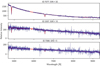 |
Fig. 1. Examples of spectra and their corresponding spexxy best fit, using high-, medium-, and low-S/N spectra for illustrative purposes. The ID number is a running number provided by SExtractor. |
3. Data analyses
The spectra extracted through the process discussed above consist of those for both member and non-member stars of Leo T. Furthermore, not all are suitable for analysis. In this section, in addition to describing the methods that we use to analyse the data, we present the steps that we took to determine which stars are likely to belong to Leo T and which can be used to obtain reliable measurements of physical parameters.
3.1. Measuring stellar velocities and abundances
The spectra that we extracted from the reduced data cube, as a general rule, have a modest S/N and spectral resolution (R ∼ 3000). As such, we adopt the same procedure as in previous articles in the series (Zoutendijk et al. 2020).
We use the spexxy full-spectrum fitting code (Husser et al. 2016) for the estimation of the physical parameters. This allows us to obtain line-of-sight velocity, metal abundance, effective temperature, and surface gravity for all stars, as long as the S/N is sufficient.
spexxy works by performing an interpolation over a grid of PHOENIX (Husser et al. 2013) model spectra, which parameterizes effective temperature, surface gravity, iron abundance ([Fe/H]), and α element abundance. Because the quality of the spectra is insufficient to allow distinction between different values of the α-element abundance ratio, we fixed the α-element abundance ratio to solar and left the other parameters free to be fitted. We proceeded this way in order to directly compare our measurements of [Fe/H] with our estimates of metallicity ([M/H]) using isochrone fitting (see Sect. 3.2). It is worth noting that the equality [M/H] = [Fe/H] only holds when the ratio of α elements to iron – denoted [α/Fe] – is zero. In the event that the stars in Leo T are enriched in α elements, we would expect to observe [M/H] > [Fe/H].
With this procedure, we were able to successfully fit 130 spectra, all of which have apparent magnitude < 24. Within the sample that was not successfully fitted, we found three emission line stars. Because the S/N values for the three spectra are sufficiently high, we concluded that their spectral type is not covered by the PHOENIX grid we use, which would lead to an unsuccessful fit. In this case, and to obtain line-of-sight velocity measurements for these stars, we adopted ULySS (Cappellari & Emsellem 2004; Koleva et al. 2009) as an alternative to obtain radial velocities. We describe ULySS in Appendix A, and compare with the results we obtain when using spexxy. However, as the results are consistent with each other, we adopt spexxy as our default method to determine the radial velocities, with the exception of the three emission line stars.
3.2. Selecting members
When selecting the Leo T member stars in our sample, we must take into account a possible contamination by Milky Way stars. As such, we estimate how many stars in our FoV are likely to be Milky Way members using the latest available Besançon model of the Milky Way (Robin et al. 2003, 2012, 2014). We simulated Milky Way star counts in the direction of Leo T and within a solid angle of 1 deg2. In the simulation, we get a total of 3083 stars when only considering apparent magnitudes between 20 and 24, which is the range of our sample. This corresponds to ≈0.86 stars in the MUSE FoV that would make it into our sample. Therefore, and from the model, we find it reasonable to expect that approximately one of the Leo T member candidates is actually a member of the Milky Way.
Furthermore, we took into account the S/N of the spectra when selecting our sample of Leo T member stars. As spexxy has been found to underestimate velocity uncertainties for spectra with a low S/N (Kamann et al. 2016), we only considered spectra with a median S/N > 3, per 1.5 Å, similar to the approach taken in Zoutendijk et al. (2020). Of the 130 spectra successfully fitted with spexxy, 56 satisfy this criterion. In addition, as the three emission-line stars also satisfy this criterion, they were also included in the sample.
Finally, in order to detect possible contamination, namely from Milky Way stars, as stated above, we performed a photometric analysis. To this end, we used F606W and F814W photometry of the public HST/ACS data, the same used to create a master list of sources. Using the photometry data, we drew a colour–magnitude diagram and matched it to isochrones from PARSEC stellar tracks and isochrones (Bressan et al. 2012). After trying different values, we assume a fixed metallicity of [M/H] = −1.6, which is consistent with the value of Weisz et al. (2012) and is also in reasonable agreement with the value found by Kirby et al. (2013). We find that this value for [M/H] leads to the best fit for our MUSE data, and we discuss this further in Sect. 4.1.
We adopted AV = 0.1 magnitudes for the interstellar extinction as a way to better align the isochrones with the data. This value is in good agreement with Schlegel et al. (1998), from which we get AVSFD = 0.0959. We find that only one of the 59 stars is inconsistent with the isochrones (having F606W − F814W ≈ 2) and was excluded. The estimated line-of-sight velocity for this star is vlos = −31.7 ± 5.5 km s−1. We consider this most likely to be a foreground M-dwarf Milky Way interloper star, which is perfectly in line with the Besançon model prediction.
Thus, we obtained a sample of 58 stars that we consider to be plausible members of Leo T. In Fig. 2 the positions of these stars are marked on the MUSE FoV. The colour–magnitude diagram referred to above, which includes these 58 stars, is shown in Fig. 3. Upon further exploration of this diagram, we identified two different populations: a younger population, with ages below 1 Gyr, and an older population with ages above 5 Gyr, which is consistent with ages as high as 10 Gyr.
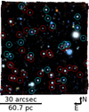 |
Fig. 2. Composite color image of Leo T based on data from the MUSE-Faint survey, created with fits2comp (https://github.com/slzoutendijk/fits2comp). We used the Johnson-Cousins filters I, R, and V to create the red, green, and blue channels of the image, respectively. The 58 stars identified in this paper as Leo T members that are located within the bounds of MUSE-Faint observations are identified with circles. As we identify two stellar populations (see Sect. 4.1), we use blue and red circles for the younger and older population, respectively. The angular and physical scales of the image are indicated in the lower left corner. Directions north and east are indicated in the lower right corner of the image. |
To make this assignment, we compared the colour–magnitude diagram of stars with a grid of isochrones based on previous results in the literature. We used PARSEC stellar tracks and isochrones (Bressan et al. 2012) to generate 10 isochrones spaced equally between 0.1 and 1 Gyr, and 7 isochrones spaced equally between 5 and 11 Gyr, all with fixed metallicity of [M/H] = −1.6. We assign each star the age of the nearest isochrone in the colour–magnitude diagram. Within our sample, we identify stars whose best fit is for ages as low as 200 Myr and others for ages as high as 10 Gyr. Due to the high age diversity in our sample, we opted to divide the stars into two samples: stars whose best fit is for ages ≤1 Gyr and stars whose best fit is for ages ≥5 Gyr.
When we fix the metallicity, there is a degeneracy between the different isochrones in certain parts of the colour–colour space. This translates into an uncertain age assignment for stars falling in this region (darker-blue colored in Fig. 3). In order to assess the sensitivity of our results below to the classification of stars in this region, we repeated the analysis while changing the assignment of stars to the young or old isochrones in this region. This did not significantly change our results, and therefore the discussion below is robust to the classification of stars in this degenerate region.
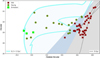 |
Fig. 3. Colour–magnitude diagram of the 58 Leo T stars detected with MUSE, plotted against PARSEC isochrones drawn for constant [Fe/H] = −1.6 and variable age. Magnitudes given are on the Vega Magnitude System. The region spanned by 0.1 − 1 Gyr isochrones is shaded in light blue with two representative isochrones shown for 0.2 and 1.0 Gyr. The region spanned by > 5 Gyr isochrones is shown in dark grey shading and a 9 Gyr isochrone is shown for illustration. At the meeting point of the two regions there is an overlap represented by a region shown in darker blue; here there is considerable degeneracy between the isochrones. The stars that were found to be consistent with the younger isochrones are shown as dark green discs, with the emission line stars shown as green squares. The stars consistent with the older isochrones are shown as red crosses. |
3.3. Distributions
While the methods described above are designed to analyse each star individually, here we describe the methods that we use to characterise Leo T as a whole. To this end, we adopt a Markov chain Monte Carlo (MCMC) method following the approach of Zoutendijk et al. (2020) in order to estimate the intrinsic mean and standard deviation of the velocity and metallicity distributions of Leo T. Here we use the logarithmic abundance relative to solar, [Fe/H], as our metallicity variable.
Here, the main assumption we make is that the velocity and metallicity distributions of the Leo T members can be well described by a Gaussian distribution. Also, we consider the possibility that there might be a contaminating population of stars belonging to the Milky Way that were not detected and whose distribution we take to be uniform in velocity across the velocity range considered, similarly to Martin et al. (2018).
We describe the MCMC method as follows. If we denote the likelihood that star i belongs to Leo T as mi, the global likelihood is given by
![$$ \begin{aligned} \mathcal{L} (\mu _{\rm int}, \sigma _{\rm int} | x_i, \epsilon _i) =&\prod _{i} \left[m_i \frac{1}{\sqrt{2\pi } \sigma _{\mathrm{obs},i}} \exp \left(-\frac{1}{2} \left(\frac{x_i - \mu _{\rm int}}{\sigma _{\mathrm{obs},i}}\right)^2\right)\right.\nonumber \\&\left. + \frac{1-m_i}{\mu _{\rm bg}^\mathrm{MAX} - \mu _{\rm bg}^\mathrm{MIN}}\right], \end{aligned} $$](/articles/aa/full_html/2023/10/aa46453-23/aa46453-23-eq13.gif)
where μint and σint are the intrinsic mean value and intrinsic dispersion of both Leo T parameters being studied. The value  is the observed velocity–metallicity dispersion for each star i, while xi denotes the measurement and ϵi the measurement uncertainty of the parameter.
For the background population, we fix the distribution by setting an upper and lower limit on the quantity considered. For the velocity, we consider  km s−1 and for the metallicity
  . For μint, we take a flat prior between 20 and 70 km s−1 for velocity and between −2.5 and 0 for [Fe/H]. We also use a flat prior on σint between 0 and 30 km s−1 and between 0 and 1 for velocity and [Fe/H], respectively. The membership likelihood is allowed to take values over the full range of 0 to 1 with a flat prior over that range, in both cases. We use emcee (Foreman-Mackey et al. 2013) to infer the posterior constraints on the parameters.
4. Results
4.1. Stellar ages
As mentioned in Sect. 3.2, we used the colour–magnitude diagram of the 58 stars considered to be members of Leo T to probe for different stellar populations. Figure 3 shows the colour–magnitude diagram for the 58 stars plotted against the PARSEC isochrones. The stars are marked with different symbols of different colours corresponding to the age group to which the stars were assigned: red crosses correspond to older stars with ages ≥5 Gyr, while green circles correspond to younger stars with ages ≤1 Gyr. The three emission-line stars are marked as green squares.
Although we divided the stars into two populations, the sample covers a wide range of ages, with some stars consistent with very old ages > 10 Gyr, while others appear to be very young, with ages of about 200 Myr or younger. The three emission line stars are just a few examples of these very young stars, which we address in more detail below. Moreover, a total of 20 stars are consistent with ages of < 1 Gyr. This is consistent with previous findings that Leo T had star formation in its recent history, making Leo T the faintest galaxy with evidence of recent star formation, partly justifying the choice of Simon (2019) to set the cut-off point for UFDs just below the luminosity of Leo T.
Furthermore, all stars are consistent with a metallicity of [M/H] = −1.6, which is in line with the existing photometric studies of Leo T (e.g. de Jong et al. 2008; Weisz et al. 2012; Clementini et al. 2012). We tried different values, but this is the one that maximises the number of stars that are consistent with the isochrones. Using this value, the older stars in the sample are consistent with ages of ∼10 Gyr. This is in line with the findings of Clementini et al. (2012), which indicates this value as an upper limit for the stellar age on Leo T. Additionally, considering a lower value for metallicity (e.g. [M/H] = −1.9) would make the redder stars in our colour–magnitude diagram inconsistent with the isochrones.
On the other hand, the value of [M/H] = −1.6 also makes the emission-line stars consistent with being on the main sequence with ages of < 500 Myr, which is consistent with the expectation that these stars have ages of < 1 Gyr. Once again, if we considered a lower value for metallicity, the best-fit isochrone for the emission line stars would correspond to an older age, which would start to be inconsistent with the expectations for these stars.
4.2. Emission line stars
The stars marked with green squares in Fig. 3 stand out not only for their youth but also for their spectra, which are shown in Fig. 4. All of them show clear Hα emission on top of a blue stellar spectrum showing Hβ in absorption.
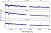 |
Fig. 4. Spectra of the three emission-line stars with the positions of the Hα and Hβ lines indicated. The ID number is a running number provided by SExtractor. |
As mentioned above, our attempt to fit the spectra with spexxy failed due to a lack of suitable templates. Therefore, we followed the approach of Roth et al. (2018) using ULySS (Cappellari & Emsellem 2004; Koleva et al. 2009) and the empirical MIUSCAT library (Vazdekis et al. 2012; see also Appendix A) to fit the stellar spectra of the three stars. We obtained the best fit for Be stars with an effective temperature of the order of Teff ∼ 104 K. It was also possible to fit their line-of-sight velocities, and these were used in the Leo T dynamics analyses discussed in Sect. 4.4.
On the basis of these results, we tentatively identify the stars as Be stars. Assuming that they are classic Be stars (e.g. Porter & Rivinius 2003; Rivinius et al. 2013), it is notable that they make up 15% of the young stars in our sample and we return to this subject in Sect. 52.
Table 3 provides positions, absolute and apparent magnitudes, and Hα line flux, equivalent width, and line width. The existing near-infrared (NIR) data for Leo T that we are aware of are not deep enough to detect the emission-line stars and therefore we are unable to measure NIR excesses, which are commonly seen in these stars (Porter & Rivinius 2003). We note that the absolute magnitudes are towards the lower end of those found by Mathew et al. (2008), which is consistent with the star population in Leo T being somewhat older than the majority surveyed in that paper.
Properties of the emission-line stars in Leo T.
We also verified that the Balmer lines are unlikely to originate in a faint ionised gas region around the Be stars. To this end, we ran some simple Cloudy models (Ferland et al. 1998) using B-star model atmospheres from Lanz & Hubeny (2007) with temperatures and luminosities spanning from B9 to B0 stars. Calculations were performed with version 17.01 of Cloudy, last described by Ferland et al. (2017). We find that, for stars with Teff < 24 kK, the measured line fluxes are too large to be explained by nebular emission from an ionised region around the stars. Taken together with the fact that the best fit for the effective temperature for these spectra is Teff < 20 kK, we conclude that a nebular origin for the lines is unlikely. This is further substantiated by the finding that star ID 7203 has a substantial line width of 167 km s−1, which is inconsistent with a nebular origin and is therefore most likely indicative of emission originating near a rapidly rotating star (see Schootemeijer et al. 2022).
4.3. Stellar metallicity
Of the 58 stars identified as Leo T members, spexxy successfully estimated the metallicity, [Fe/H], for 55 stars (it failed for the three emission line stars). Figure 5 shows the histogram of the metallicity estimates. To quantify this distribution, we adopt the model described in Sect. 3.3. Therefore, we assume that the underlying metallicity distribution is a Gaussian, which appears to be a reasonable approximation in this case. We note that stars in the wings of the distribution typically have low-S/N spectra. Furthermore, the stars with measurements of [Fe/H] < −2.5 have higher uncertainties on [Fe/H], as their spectra present almost no lines. We further explore the impact of these uncertainties in Appendix B.
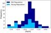 |
Fig. 5. Distribution of the metallicity ([Fe/H]) of 55 Leo T stars estimated using spexxy. The younger population, consisting of 17 stars, is represented with a lighter colour. |
By fitting the model to the distribution, we find a mean value of [Fe/H] = −1.53 ± 0.05 and a dispersion of σ[Fe/H] = 0.21 ± 0.06. The fit also considers that 99% of the members of the sample are consistent with the model. The resulting corner plot of this MCMC fitting is shown in Fig. 6.
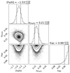 |
Fig. 6. Corner plot for the MCMC metallicity fit using a sample of 55 stars. We show the mean metallicity, μu, dispersion σu, and fraction of stars consistent with the model. |
The results are consistent with those obtained from our photometric analyses, which is expected considering we used [α/Fe] = 0 in both measurements. However, as stated above, if we change the fixed value for [α/Fe] in our fit with spexxy we get different values accordingly.
To detect differences in metallicity between the young and old populations, we repeated the analysis separately for each population. Although the results appear to be consistent with each other (see Appendix B), we draw attention to the fact that the sample of the young population consists only of 17 stars, which is too small to put reliable constraints on the metallicity for the young population. Nevertheless, the constraints for the younger population are consistent with the results for the older population, although they favour a somewhat lower metallicity for the younger population. We discuss this further in Appendix B.
4.4. Stellar kinematics
Here, we start by discussing the overall kinematics for all the stars with velocity measurements, combining MUSE and literature data.
As such, here we also used 17 of the 19 stars with kinematics measurements from Simon & Geha (2007). Two stars were excluded because they overlap between the samples. Additionally, our line-of-sight measurements and those from the literature are consistent with each other for the two stars when considering the uncertainties.
Therefore, the total sample for the kinematic analysis consists of 75 stars, which is the same sample presented by Zoutendijk et al. (2021b). The velocity histogram for these stars is displayed in Fig. 7.
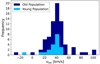 |
Fig. 7. Histogram of the line-of-sight velocities for Leo T members (75 stars), measured by fitting their spectra with spexxy (55 stars), ULySS (3 stars), and adding the results of Simon & Geha (2007) (17 stars). The lighter colour corresponds to the younger population in the MUSE sample. |
To the data, we fit the model described in Sect. 3.3 using MCMC and the resulting corner plot is shown in Fig. 8. We find a mean velocity of  km s−1, and an intrinsic velocity dispersion of
  km s−1 with 99% of the sample consistent with the model. The results are in agreement with both the measurements made by Simon & Geha (2007) and the H I velocity and velocity dispersion measurements reported by Adams & Oosterloo (2018).
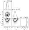 |
Fig. 8. Corner plot for the MCMC velocity fit using the entire sample of 75 stars. We show the mean value vlos, dispersion σv, and fraction of stars consistent with the model. |
We note here that, as the analysis deconvolves from the uncertainties on the velocities, it is important that the MUSE and Simon & Geha (2007) measurement uncertainties are on the same scale. To verify this, we ran the MCMC with a slightly modified version of the model in Eq. (1) where we added a scale factor for the uncertainties of the spexxy measurements. Marginalising this, we find that this scale factor is consistent with one, indicating that the measurement uncertainty estimates in the two datasets are consistent.
Similarly to what we did in Sect. 4.3, we explored any possible kinematical difference between the young and old stellar populations in Leo T. We repeated the analysis with the sample divided into two sets: one with 20 stars that are consistent with ages of ≤1 Gyr and another with 55 stars consistent with ages of ≥1 Gyr. Here, we considered the entire sample of Simon & Geha (2007) to be composed of old stars.
Naturally, both sets were fitted with the MCMC method described above. This time, for the younger sample we get a mean value of  km s−1, a velocity dispersion of
  km s−1, with 96% of the sample being consistent with the model. For the older sample, we got a mean value of
  km s−1, a velocity dispersion of
  km s−1, with 99% of the sample being consistent with the model. The corner plots for these results are shown in Fig. 9 for the young stars, and Fig. 10 for the old stars.
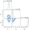 |
Fig. 9. Corner plot for the MCMC velocity fit using the sample of 20 stars with ages of ≤1 Gyr. We show the mean value vlos, dispersion σv, and fraction of stars consistent with the model. |
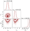 |
Fig. 10. Corner plot for the MCMC velocity fit using the sample of 55 stars with ages of ≥1 Gyr, including the data from Simon & Geha (2007). We show the mean value vlos, dispersion σv, and fraction of stars consistent with the model. |
As only the set of older stars includes data from Simon & Geha (2007), we also repeated the analysis for the older stars but considering only the 38 MUSE stars. The estimated intrinsic velocity dispersion is almost the same as before, but the estimated mean velocity increases by ∼3 km s−1. The corner plot for these results is shown in Fig. 11. Either way, the younger stars show a significantly smaller velocity dispersion than the older stars.
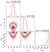 |
Fig. 11. Corner plot for the MCMC velocity fit using the sample of 38 stars with ages of ≥1 Gyr within the MUSE FoV. We show the mean value vlos, dispersion σv, and fraction of stars consistent with the model. |
We now compare the differences in kinematics between young and old stars with what was found by Adams & Oosterloo (2018) when analysing the H I kinematics of warm and cold neutral gas (see also Table 1). This comparison can be seen in Figs. 12 and 13, where we show the measured values stated above and the measurements of Adams & Oosterloo (2018) that are displayed in Table 1.
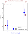 |
Fig. 12. Comparison between stellar velocity dispersion of this work and neutral gas velocity dispersion from Adams & Oosterloo (2018). For the older stellar population, we present two values: estimation using only the MUSE sample and estimation using MUSE + literature sample from Simon & Geha (2007). |
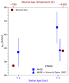 |
Fig. 13. Comparison between stellar velocity of this work and neutral gas velocity from Adams & Oosterloo (2018). For the older stellar population, we present two values: estimation using only the MUSE sample and estimation using MUSE + literature sample from Simon & Geha (2007). |
We find a good match when comparing the velocity dispersion of the young population with the cold component of the H I gas, and between the kinematics of old Leo T stars and the warm component of the H I gas, as shown in Fig. 12. The most natural explanation for this is that the current cold H I gas is representative of the gas from which this young population of stars formed and that these stars have not yet been heated dynamically to the velocity dispersion of the halo. On the other hand, assuming that the warm H I gas has remained in the system for a significant time, both the WNM and the old stars are accurately tracking the gravitational potential of the galaxy.
We also compare the mean velocity of both populations of stars with both components of the neutral gas (see Fig. 13). Here, and using the entire sample, we find negligible differences between the mean velocity of the young and old populations, which contrasts with the difference in the mean velocity found for the cold and warm components of the H I gas.
Nevertheless, this is not the case when the analysis is performed using only the MUSE stars. In that case, we find a difference of ∼3 km s−1 between the mean velocity of old and young stars. We are unable to identify the reason for the offset. We note that the telluric correction applied by Simon & Geha (2007) is different from the way our velocity estimates are made. Also, the spatial distribution of the stars in the Simon & Geha (2007) sample is different from that of the MUSE sample, as MUSE observations target the innermost stars of Leo T.
4.5. No extended emission line sources
The presence of young stars raises the question of whether there is ongoing star formation in Leo T. The MUSE data are particularly well-suited for this as they allow for the construction of very deep narrow-band images over lines of interest.
Figure 14 shows the narrow-band images over Hα and O[III]5007. These were created by weighting a Gaussian centred on the wavelength of the lines adjusted by the line-of-sight velocity of Leo T, and with a velocity width of σ = 70 km s−1. We sum this up over ±5σ after removing the background. We estimate the background as the median over ±100 Å excluding the ±5σ region.
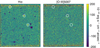 |
Fig. 14. Narrow-band images over Hα (left) and O[III]5007 (right). In the left-hand panel the three emission line stars are easily seen, but no evidence is found of extended emission in either Hα or O[III]5007. |
The Hα image shows a number of dark sources. These are stars in the FoV showing Hα absorption close to the velocity of Leo T. The three bright sources circled in white are the three emission line stars discussed above.
There is no sign of extended emission in either image. To estimate a detection limit, we calculated an empirical noise estimate by randomly distributing 100 apertures over the narrow-band images and calculating the median absolute deviation of the measured median level. This leads to a 1σ limit for Hα of 0.99 × 10⁻²⁰ and 24.89 × 10⁻²⁰ per pixel and per squared arcsecond, respectively, in units of erg s−1 cm−2 for a single line with line width 70 km s−1. For O[III]5007, the values are 1.05 × 10⁻²⁰ and 26.29 × 10⁻²⁰ respectively.
We repeated the calculation using a data cube not corrected with ZAP to check for differences. We get a 1σ limit for Hα of 1.04 × 10⁻²⁰ and 25.92 × 10⁻²⁰ per pixel and per arcsecond squared, respectively, in units of erg s−1 cm−2 for a single line with line width 70 km s−1. For O[III]5007, the values are 1.11 × 10⁻²⁰ and 27.73 × 10⁻²⁰ respectively. Therefore, we conclude that the use of ZAP to remove residual sky signatures does not affect our results here.
We convert the Hα flux into an upper limit on star formation rate (SFR) using the LHα–SFR relation derived by Kennicutt (1998). We get a SFR ≈ 4 × 10⁻¹¹ M⊙ yr−1 per arcsec, corresponding to a SFR ∼ 10−11 M⊙ yr−1 pc−2. It is worth noting that the SFR calibration assumes solar metallicity and a fully populated initial mass function (IMF), neither of which are likely to be satisfied in Leo T. However, even allowing for this, the SFR upper limit is extremely low, which is an indication of the lack of ongoing star formation in Leo T.
5. Discussion
We find that Leo T has two stellar populations that have significantly different age and dynamics when compared to the neutral gas. However, the metallicity of the two populations appears to be nearly identical. We also see that the young population, despite its low metallicity, contains emission-line Be stars with properties comparable to those found in surveys of more metal-rich populations (Porter & Rivinius 2003). Despite the presence of young stars, we do not detect extended emission-line sources. Here, we discuss the results and compare them with those from the literature.
5.1. Metallicity and star formation
The most immediate interpretation of the lack of extended emission line sources is that star formation has ended. Weisz et al. (2012), based on the stellar photometry, argue that star formation ended about 25 Myr ago, which is consistent with the lack of extended emission from any H II region. Therefore, our observations corroborate the picture presented by Weisz et al. (2012) of essentially no star formation in Leo T in the last ∼25 Myr. This is consistent with recent models that suggest that star formation in low-mass galaxies should be bursty with short quiescent periods (e.g. Collins & Read 2022).
This is also consistent with the low dispersion in [Fe/H] in Leo T, which implies that all stars have approximately the same metallicity of [Fe/H] ∼ −1.6. This can be compared with the findings of Weisz et al. (2012). We do see similar behaviour in other dwarf galaxies (e.g. Aquarius Cole et al. 2014), and theoretical models have predicted that metals can escape from low-mass dwarfs due to stellar feedback, keeping [Fe/H] approximately constant (Jeon et al. 2017; Emerick et al. 2018), which is also enabled by a bursty star formation. Nevertheless, this appears to happen only after an initial chemical evolution, which we do not see in Leo T. We measure the same metallicity for stars consistent with ages as low as ∼200 Myr and as high as ∼10 Gyr, which is rather surprising given the interpretation of Leo T as a galaxy with near-constant star formation over cosmic time.
Additionally, a value of [Fe/H] ∼ −1.6 makes the older stars of Leo T quite metal-rich compared to what we see in other dwarfs (Jeon et al. 2017). As we cannot confirm the age of the stars, due to the degeneracy between the different isochrones, there is the possibility that these stars are younger than is indicated by our fit. We could be missing an older and more metal-poor population in our analysis, which could also explain why our measured metallicity is not identical to the value of Simon (2019), assuming that this difference does not result from differences in calibration or data processing. However, there is no clear reason as to why we would not detect such population, considering that we are observing the Leo T field. It is worth noting that a significant portion of our sample has been removed due to low S/N. Typically, these stars are of low luminosity, which may indicate that they are quite old and, presumably, have low metal content. Therefore, it is possible that the members of the population we assume is missing could be among the stars that were rejected due to low S/N. To explore this possibility, we look at the sample of 194 spectra that were not used in our analysis due to the S/N cut or because of a failed spexxy fit. Naturally, these spectra share a commonality in that they are very faint. In the colour–magnitude space, they generally fall between F814W ∼ 24 and 26 and between F606W − F814W ∼ 0 and 0.6, which suggests the presence of multiple age and/or metallicity populations. Nonetheless, due to the faintness of those objects (and respective low S/N) we are unable to fit their spectra and verify the hypotheses that an older and more metal-poor population exists. We draw attention to the fact that these results are in line with the observations of Weisz et al. (2012).
Subsequently, we cannot discard the possibility that the older Leo T stars present a value of [Fe/H] ∼ −1.6, which would indicate that Leo T was chemically enriched before starting to produce stars. Deeper observations are needed to solve this dilemma.
5.2. Recent star formation and link to the CNM
In Adams & Oosterloo (2018), the fact that Leo T has a significant amount of its H I mass in the CNM phase but a low star-formation efficiency compared to other dwarf galaxies was discussed in some detail. The authors highlighted a number of possible explanations, but emphasised in particular the possibility that the formation of the CNM is recent and connected to the infall of Leo T into the Milky Way halo and is therefore less connected to the star formation in Leo T.
However, here we find that the CNM and the young stars in Leo T have comparable dynamical properties, and therefore a close link between the two appears natural. Both have significantly smaller velocity dispersions than the WNM and the older stars. In this context, it is natural to ask how long it would take for the young stars or the CNM to approach the dynamical state of the older stars.
We can estimate the relaxation time of the system, if we write it as (Spitzer & Hart 1971)
where D(Δv2) is the diffusion coefficient and has the greatest impact, which for a spherical system and an isotropic Maxwellian velocity distribution for both young and old stars can be written as
where ma is the mass of the younger stars and σ their velocity dispersion, lnΛ is the Coulomb logarithm and  , with v denoting the typical velocity of the older stellar component. We approximate the Coulomb logarithm as
where we take R to be the half-light radius of Leo T (see Table 1) and σold to be the velocity dispersion of the old component. The IMF-weighted average mass of the old and young population will differ, but the difference is modest for the ages relevant here, and so for order-of-magnitude estimates we can set them equal to 0.3 M⊙.
Taking the velocity dispersions given in Sect. 4.4, and the density profile and mass-to-light ratio presented in Zoutendijk et al. (2021b), we estimate relaxation times of > 1013 yr. While the relaxation time could be reduced if dark matter is made up of massive compact halo objects (MACHOs), these latter would need to have masses that are excluded by other constraints (e.g. Brandt 2016; Zoutendijk et al. 2020) in order to bring the relaxation time below a Hubble time.
Therefore, we can conclude that the kinematics of the young population is likely a fair reflection of the kinematics of the gas it formed out of. As the young stellar population shows very similar kinematics to the CNM, the natural inference is that the most recent star formation in Leo T originated from gas whose remnants now make up the CNM. However, this also means that the overall velocity dispersion that we find above, which includes contributions from the young population whose kinematics may not yet be fully relaxed, may not reflect the true gravitational potential of Leo T. Therefore, the velocity dispersion of the older stars may provide a more reliable probe of the gravitational potential of the system.
The different kinematics of the CNM and WNM, and more precisely the different mean velocity, might imply an external origin for the CNM, through accretion for example. Another result that would support the extragalactic accretion argument is that of the metallicity of the younger population of Leo T. The fact that the younger population could have a lower metallicity than the older stars might imply that the younger stars formed from gas less chemically enriched than that of the gas from which the older stars formed; an external origin for this gas would explain this observation.
Another natural explanation is related to the infall of Leo T into the Milky Way circumgalactic medium. Indeed, the ram pressure affects the hot, more extended gas more rapidly than the cool gas (Emerick et al. 2016), and this could explain the difference in kinematics between the two components of the gas. This would lead to changes in the internal structure of the gas, which would also explain the recent quench in star formation in Leo T.
5.3. Be stars in metal-poor environments
Turning now to the properties of young stars, in particular the emission-line Be stars identified in Sect. 4.2, their presence offers some insight into the formation of stars at low metallicity. We find that 15% of the stars classified as young show Hα in emission, which can be compared to the Milky Way study of Mathew et al. (2008), who reported rates at a level of 10%–20% in stellar clusters. Schootemeijer et al. (2022), who present a study of Be stars in metal-poor environments down to one-tenth of solar, find OBe fractions of between 0.2 and 0.3 when limited to main sequence stars. This is consistent with what is found in Leo A, where Gull et al. (2022) recently reported the spectroscopic detection of Be stars at a metallicity of one-tenth of solar. Meanwhile, Leščinskaitė et al. (2022) found that, for Leo A, the emission-line stars account for up to ∼15% of the blue helium-burning (BHeB) stars. Similar values are also found in other metal-poor environments, such as NGC 2345 with [Fe/H] = −0.28 (Alonso-Santiago et al. 2019).
As the presence of emission lines in these stars is thought to be linked to high rotational velocities, these findings suggest that extremely rapidly rotating massive stars are common in low-metallicity environments (Schootemeijer et al. 2022). Leo T pushes this down to 1/30 solar metallicity, and although the number of stars is too small to place strong constraints, the fraction of emission line stars on the main sequence in Leo T is high. Coupled with the large velocity width seen in the Hα line, this supports the conclusions of Schootemeijer et al. (2022).
6. Conclusions
We present a MUSE study of Leo T, one of the galaxies with the lowest mass showing signs of recent star formation. We were able to increase the number of spectroscopically observed Leo T stars from 19 to 75, which led to the following results.
By combining the MUSE data with HST photometry and performing a photometric analysis, we identified two stellar populations – in agreement with previous results in the literature – with a wide range of stellar ages, from as low as 200 Myr to as high as 10 Gyr. We divide the population into two samples such that the younger population shows consistency with ages of < 500 Myr, while the older population shows ages of > 5 Gyr. Within the younger population, we identified three emission-line Be stars, corresponding to 15% of the stars classified as young. This is in line with results for the Milky Way, although these stars show much lower metallicities, and our findings therefore suggest a substantial number of rapidly rotating young stars at 1/30 solar metallicity.
The presence of young stars could indicate that there is ongoing star formation in Leo T, but we find no evidence of the existence of extended emission-line regions to a surface brightness of < 1 × 10⁻²⁰ erg s−1 cm−2 arcsec−2, which corresponds to an upper limit SFR ∼ 10−11 M⊙ yr−1 pc−2. Therefore, we conclude that star formation has ended, which is consistent with Weisz et al. (2012), who conclude that there has been no star formation in the last ∼25 Myr.
By fitting the MUSE spectra, we obtained a metallicity of [Fe/H] = −1.53 ± 0.05, which is in good agreement with our photometric analysis, assuming that [α/Fe] = 0. We also find a metallicity dispersion of σ[Fe/H] = 0.21 ± 0.06. The low dispersion in [Fe/H] shows that all stars have very similar metallicity, implying that Leo T underwent almost no evolution throughout its history, which is puzzling considering the claimed extended star formation history and age range (from 200 Myr up to 10 Gyr) of this dwarf. This seems to indicate that a large fraction of metals were ejected, namely due to stellar feedback. This has been predicted by theoretical models that also show that star formation in low-mass galaxies should be bursty with short quiescent periods, and these findings support that conclusion.
Using the sample of 75 stars, we measured the kinematics of Leo T stars in the most robust kinematic study of this dwarf to date. We find a velocity dispersion of  km s−1. This result is consistent with previous estimates of the kinematics of stars, but, more importantly here, it is also concordant with the measured H I gas kinematics. Interestingly, when splitting the sample into young and old stars, we find that they have different kinematics. We find a velocity dispersion of
  km s−1 for the younger population and a much higher velocity dispersion of
  km s−1 for the older population. This means that the cold component of the H I gas and the young stars in Leo T have comparable kinematics.
We estimate the time that it would take for young stars or the cold component of H I gas to approach the dynamical state of older stars to be higher than the Hubble time, which directly links the most recent star formation in Leo T to the cold component of the H I gas.
Acknowledgments
D.V. and J.B. acknowledge support by Fundação para a Ciência e a Tecnologia (FCT) through the research grants UID/FIS/04434/2019, UIDB/04434/2020, UIDP/04434/2020. D.V. acknowledges support from the Fundação para a Ciência e a Tecnologia (FCT) through the Fellowship 2022.13277.BD. J.B. acknowledges financial support from the Fundação para a Ciência e a Tecnologia (FCT) through national funds PTDC/FIS-AST/4862/2020 and work contract 2020.03379.CEECIND. S.L.Z. acknowledges support by The Netherlands Organisation for Scientific Research (NWO) through a TOP Grant Module 1 under project number 614.001.652. S.K. acknowledges funding from UKRI in the form of a Future Leaders Fellowship (grant no. MR/T022868/1). P.M.W. acknowledges support by the BMBF from the ErUM program (project VLT-BlueMUSE, grant 05A20BAB). Based on observations made with ESO Telescopes at the La Silla Paranal Observatory under programme IDs 0100.D-0807, 0101.D-0300, 0102.D-0372 and 0103.D-0705. This research has made use of Astropy (Astropy Collaboration 2013, 2018), corner.py (Foreman-Mackey et al. 2013), matplotlib (Hunter 2007), NASA’s Astrophysics Data System Bibliographic Services, NumPy (Harris et al. 2020), SciPy (Virtanen et al. 2020).
References
- Adams, E. A. K., & Oosterloo, T. A. 2018, A&A, 612, A26 [NASA ADS] [CrossRef] [EDP Sciences] [Google Scholar]
- Alonso-Santiago, J., Negueruela, I., Marco, A., et al. 2019, A&A, 631, A124 [NASA ADS] [CrossRef] [EDP Sciences] [Google Scholar]
- Applebaum, E., Brooks, A. M., Christensen, C. R., et al. 2021, ApJ, 906, 96 [NASA ADS] [CrossRef] [Google Scholar]
- Astropy Collaboration (Robitaille, T. P., et al.) 2013, A&A, 558, A33 [NASA ADS] [CrossRef] [EDP Sciences] [Google Scholar]
- Astropy Collaboration (Price-Whelan, A. M., et al.) 2018, AJ, 156, 123 [Google Scholar]
- Bacon, R., Accardo, M., Adjali, L., et al. 2010, Proc. SPIE, 7735, 773508 [Google Scholar]
- Bacon, R., Conseil, S., Mary, D., et al. 2017, A&A, 608, A1 [NASA ADS] [CrossRef] [EDP Sciences] [Google Scholar]
- Bertin, E., & Arnouts, S. 1996, A&AS, 117, 393 [NASA ADS] [CrossRef] [EDP Sciences] [Google Scholar]
- Bocquet, S., & Carter, F. W. 2016, J. Open Source Softw., 1, 24 [NASA ADS] [CrossRef] [Google Scholar]
- Brandt, T. D. 2016, ApJ, 824, L31 [NASA ADS] [CrossRef] [Google Scholar]
- Bressan, A., Marigo, P., Girardi, L., et al. 2012, MNRAS, 427, 127 [NASA ADS] [CrossRef] [Google Scholar]
- Brook, C. B., & Cintio, A. D. 2015, MNRAS, 453, 2133 [NASA ADS] [CrossRef] [Google Scholar]
- Bullock, J. S., & Boylan-Kolchin, M. 2017, ARA&A, 55, 343 [Google Scholar]
- Cappellari, M., & Emsellem, E. 2004, PASP, 116, 138 [Google Scholar]
- Cintio, A. D., Brook, C. B., Macciò, A. V., et al. 2013, MNRAS, 437, 415 [Google Scholar]
- Clementini, G., Cignoni, M., Ramos, R. C., et al. 2012, ApJ, 756, 108 [NASA ADS] [CrossRef] [Google Scholar]
- Cole, A. A., Weisz, D. R., Dolphin, A. E., et al. 2014, ApJ, 795, 54 [Google Scholar]
- Collins, M. L. M., & Read, J. I. 2022, Nat. Astron., 6, 647 [NASA ADS] [CrossRef] [Google Scholar]
- de Jong, J. T. A., Harris, J., Coleman, M. G., et al. 2008, ApJ, 680, 1112 [NASA ADS] [CrossRef] [Google Scholar]
- Emerick, A., Low, M.-M. M., Grcevich, J., & Gatto, A. 2016, ApJ, 826, 148 [NASA ADS] [CrossRef] [Google Scholar]
- Emerick, A., Bryan, G. L., Low, M.-M. M., et al. 2018, ApJ, 869, 94 [NASA ADS] [CrossRef] [Google Scholar]
- Ferland, G. J., Korista, K. T., Verner, D. A., et al. 1998, PASP, 110, 761 [Google Scholar]
- Ferland, G. J., Chatzikos, M., Guzmán, F., et al. 2017, Rev. Mex. Astron. Astrofis., 53, 385 [NASA ADS] [Google Scholar]
- Foreman-Mackey, D., Hogg, D. W., Lang, D., & Goodman, J. 2013, PASP, 125, 306 [Google Scholar]
- Gull, M., Weisz, D. R., Senchyna, P., et al. 2022, ApJ, 941, 206 [NASA ADS] [CrossRef] [Google Scholar]
- Gutcke, T. A., Pfrommer, C., Bryan, G. L., et al. 2022, ApJ, 941, 120 [NASA ADS] [CrossRef] [Google Scholar]
- Harris, C. R., Millman, K. J., van der Walt, S. J., et al. 2020, Nature, 585, 357 [NASA ADS] [CrossRef] [Google Scholar]
- Hunter, J. D. 2007, Comput. Sci. Eng., 9, 90 [NASA ADS] [CrossRef] [Google Scholar]
- Husser, T.-O., Wende-von Berg, S., Dreizler, S., et al. 2013, A&A, 553, A6 [NASA ADS] [CrossRef] [EDP Sciences] [Google Scholar]
- Husser, T.-O., Kamann, S., Dreizler, S., et al. 2016, A&A, 588, A148 [NASA ADS] [CrossRef] [EDP Sciences] [Google Scholar]
- Irwin, M. J., Belokurov, V., Evans, N. W., et al. 2007, ApJ, 656, L13 [NASA ADS] [CrossRef] [Google Scholar]
- Jeon, M., Besla, G., & Bromm, V. 2017, ApJ, 848, 85 [NASA ADS] [CrossRef] [Google Scholar]
- Kamann, S., Wisotzki, L., & Roth, M. M. 2013, A&A, 549, A71 [NASA ADS] [CrossRef] [EDP Sciences] [Google Scholar]
- Kamann, S., Husser, T.-O., Brinchmann, J., et al. 2016, A&A, 588, A149 [NASA ADS] [CrossRef] [EDP Sciences] [Google Scholar]
- Kennicutt, R. C. 1998, ARA&A, 36, 189 [NASA ADS] [CrossRef] [Google Scholar]
- Kirby, E. N., Simon, J. D., Geha, M., Guhathakurta, P., & Frebel, A. 2008, ApJ, 685, L43 [NASA ADS] [CrossRef] [Google Scholar]
- Kirby, E. N., Lanfranchi, G. A., Simon, J. D., Cohen, J. G., & Guhathakurta, P. 2011, ApJ, 727, 78 [Google Scholar]
- Kirby, E. N., Cohen, J. G., Guhathakurta, P., et al. 2013, ApJ, 779, 102 [Google Scholar]
- Koleva, M., Prugniel, P., Bouchard, A., & Wu, Y. 2009, A&A, 501, 1269 [CrossRef] [EDP Sciences] [Google Scholar]
- Lanz, T., & Hubeny, I. 2007, ApJS, 169, 83 [CrossRef] [Google Scholar]
- Leščinskaitė, A., Stonkutė, R., & Vansevičius, V. 2022, A&A, 660, A79 [NASA ADS] [CrossRef] [EDP Sciences] [Google Scholar]
- Martin, N. F., Collins, M. L. M., Longeard, N., & Tollerud, E. 2018, ApJ, 859, L5 [NASA ADS] [CrossRef] [Google Scholar]
- Mathew, B., Subramaniam, A., & Bhatt, B. C. 2008, MNRAS, 388, 1879 [NASA ADS] [CrossRef] [Google Scholar]
- Navarro, J. F., Eke, V. R., & Frenk, C. S. 1996, MNRAS, 283, L72 [NASA ADS] [Google Scholar]
- Orkney, M. D. A., Read, J. I., Rey, M. P., et al. 2021, MNRAS, 504, 3509 [NASA ADS] [CrossRef] [Google Scholar]
- Porter, J. M., & Rivinius, T. 2003, PASP, 115, 1153 [Google Scholar]
- Read, J. I., Agertz, O., & Collins, M. L. M. 2016, MNRAS, 459, 2573 [NASA ADS] [CrossRef] [Google Scholar]
- Read, J. I., Walker, M. G., & Steger, P. 2019, MNRAS, 484, 1401 [NASA ADS] [CrossRef] [Google Scholar]
- Regis, M., Taoso, M., Vaz, D., et al. 2021, Phys. Lett. B, 814, 136075 [NASA ADS] [CrossRef] [Google Scholar]
- Rey, M. P., Pontzen, A., Agertz, O., et al. 2020, MNRAS, 497, 1508 [NASA ADS] [CrossRef] [Google Scholar]
- Rivinius, T., Carciofi, A. C., & Martayan, C. 2013, A&ARv, 21, A69 [NASA ADS] [CrossRef] [Google Scholar]
- Robin, A. C., Reylé, C., Derrière, S., & Picaud, S. 2003, A&A, 409, 523 [NASA ADS] [CrossRef] [EDP Sciences] [Google Scholar]
- Robin, A. C., Marshall, D. J., Schultheis, M., & Reylé, C. 2012, A&A, 538, A106 [NASA ADS] [CrossRef] [EDP Sciences] [Google Scholar]
- Robin, A. C., Reylé, C., Fliri, J., et al. 2014, A&A, 569, A13 [CrossRef] [EDP Sciences] [Google Scholar]
- Roth, M. M., Sandin, C., Kamann, S., et al. 2018, A&A, 618, A3 [NASA ADS] [CrossRef] [EDP Sciences] [Google Scholar]
- Ryan-Weber, E. V., Begum, A., Oosterloo, T., et al. 2008, MNRAS, 384, 535 [NASA ADS] [CrossRef] [Google Scholar]
- Schlegel, D. J., Finkbeiner, D. P., & Davis, M. 1998, ApJ, 500, 525 [Google Scholar]
- Schootemeijer, A., Lennon, D. J., Garcia, M., et al. 2022, A&A, 667, A100 [NASA ADS] [CrossRef] [EDP Sciences] [Google Scholar]
- Simon, J. D. 2019, ARA&A, 57, 375 [NASA ADS] [CrossRef] [Google Scholar]
- Simon, J. D., & Geha, M. 2007, ApJ, 670, 313 [NASA ADS] [CrossRef] [Google Scholar]
- Soto, K. T., Lilly, S. J., Bacon, R., Richard, J., & Conseil, S. 2016, MNRAS, 458, 3210 [Google Scholar]
- Spitzer, L., Jr., & Hart, M. H. 1971, ApJ, 164, 399 [NASA ADS] [CrossRef] [Google Scholar]
- Vazdekis, A., Ricciardelli, E., Cenarro, A. J., et al. 2012, MNRAS, 424, 157 [Google Scholar]
- Virtanen, P., Gommers, R., Oliphant, T. E., et al. 2020, Nat. Meth., 17, 261 [Google Scholar]
- Walker, M. G., & Peñarrubia, J. 2011, ApJ, 742, 20 [CrossRef] [Google Scholar]
- Weilbacher, P. M., Palsa, R., Streicher, O., et al. 2020, A&A, 641, A28 [NASA ADS] [CrossRef] [EDP Sciences] [Google Scholar]
- Weisz, D. R., Zucker, D. B., Dolphin, A. E., et al. 2012, ApJ, 748, 88 [CrossRef] [Google Scholar]
- Wolf, J., Martinez, G. D., Bullock, J. S., et al. 2010, MNRAS, 406, 1220 [NASA ADS] [Google Scholar]
- Zoutendijk, S. L., Brinchmann, J., Boogaard, L. A., et al. 2020, A&A, 635, A107 [NASA ADS] [CrossRef] [EDP Sciences] [Google Scholar]
- Zoutendijk, S. L., Brinchmann, J., Bouché, N. F., et al. 2021a, A&A, 651, A80 [NASA ADS] [CrossRef] [EDP Sciences] [Google Scholar]
- Zoutendijk, S. L., Júlio, M. P., Brinchmann, J., et al. 2021b, arXiv e-prints [arXiv:2112.09374] [Google Scholar]
Appendix A: ULySS
To check the robustness of the velocity estimation method we used in this work, we follow the approach of Roth et al. (2018), using ULySS (Cappellari & Emsellem 2004; Koleva et al. 2009) and the empirical MIUSCAT library (Vazdekis et al. 2012) to fit the stellar spectra, as an alternative method to measure the radial velocity. We did this in two different ways: by fitting a single stellar spectrum from the library to the full spectrum and using this to get vlos; and by fitting multiple reference spectra to the observed spectrum and using this composite spectrum to get vlos. The composite spectrum is created by combining different spectra from the library in order to achieve a best fit. This method could in particular be useful for identifying observed spectra that are a composite of the spectra of multiple objects, e.g. from binaries.
As such, we fit each individual spectrum twice, and we consider the result corresponding to the best fit. We compare the results of ULySS and spexxy for the sample of 55 stars (as spexxy failed to fit the emission-line star spectra) and look for discrepancies.
Figure A.1 shows the difference in the radial velocity estimates between spexxy and ULySS against the measured S/N. The displayed error is determined by summing in quadrature the respective measurement uncertainties. The stars which ULySS best fit employ reference spectra of multiple spectral types (composite spectra) are shown in orange. From the results, it is clear that both measurements are consistent with each other within the errors. For a higher S/N, the difference in both measurements is effectively zero. We do see a larger dispersion for lower S/N values, which is to be expected, but this is compensated for by the larger uncertainties.
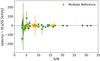 |
Fig. A.1. Difference between spexxy and ULySS velocity measurements as a function of S/N. The displayed error was determined by summing the respective measurement uncertainties in quadrature. The stars for which the ULySS best-fit run used multiple reference spectra are displayed as orange squares. A horizontal dashed line at zero is also shown. |
Therefore, we concluded that the two velocity estimation methods give consistent results and adopted spexxy as the main method to fit the spectra in the analysis. As the spexxy runs failed for the emission line spectra, we used the ULySS measurements for these objects in the kinematic analysis.
We note that ULySS favoured a complex spectrum fit for 15 stars, which might indicate unresolved binaries, but we mention here that the final spectra are averages over several independent epochs, and therefore they are likely to be less affected by binary motions than single-epoch spectra, and we do not attempt to correct for this here.
Appendix B: [Fe/H] Analysis complement
Here we discuss the metallicity analysis when performed separately for the young and old population. From the sample of 55 stars with [Fe/H] measured spectroscopically, 17 are members of the young population. For these two samples, we fit the MCMC model described in Section 3.3. As the sample for the young population is too small, the constraints have a large uncertainty. The results are shown in Figure B.1. This plot was generated using the pygtc package (Bocquet & Carter 2016). We see that, for the younger population, an equal or lower metallicity is preferred in comparison to the one preferred for the older population. However, the uncertainty is too high to yield a firm result.
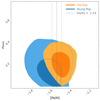 |
Fig. B.1. Plot of the covariance distribution of the mean [Fe/H] and [Fe/H] dispersion drawn from the MCMC analysis. The result for the young and old population is plotted in blue and orange, respectively. The darker shade symbolises the middle 68% of the distribution. The dashed lines represent the mean [Fe/H] and the uncertainty obtained by fitting the entire sample with the same MCMC method. |
In order to better understand the results, we plot the [Fe/H] measurements as a function of the uncertainty in Figure B.2. We get some measurements that we consider to be outliers, with measured [Fe/H] < −2.5. These values, if real, are very surprising, in particular because most of them are for young stars. However, as the uncertainty is quite high for lower metallicity cases, it is not possible to have a definite conclusion. Furthermore, we repeated the MCMC analysis by removing the outliers and the results were unchanged, which means that, due to the large uncertainty, these measurements do not contribute significantly to the success of the fit. If these measurements are inaccurate, the outliers can be explained by the fact that these young stars barely have any metal lines in the MUSE spectral range. Therefore, spexxy can wander off in the metallicity space, because changes in [Fe/H] do not affect the fit. There is also the possibility that the parameter space is not well covered by the PHOENIX grid for these types of young stars, contributing to a poorer fit.
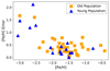 |
Fig. B.2. Plot of the measured [Fe/H] and [Fe/H] uncertainty for the sample of 55 stars, using spexxy. The sample is divided into two, representing the young and old population in blue and orange, respectively. |
All Tables
All Figures
|
Fig. 1. Examples of spectra and their corresponding spexxy best fit, using high-, medium-, and low-S/N spectra for illustrative purposes. The ID number is a running number provided by SExtractor. |
| In the text | |
|
Fig. 2. Composite color image of Leo T based on data from the MUSE-Faint survey, created with fits2comp (https://github.com/slzoutendijk/fits2comp). We used the Johnson-Cousins filters I, R, and V to create the red, green, and blue channels of the image, respectively. The 58 stars identified in this paper as Leo T members that are located within the bounds of MUSE-Faint observations are identified with circles. As we identify two stellar populations (see Sect. 4.1), we use blue and red circles for the younger and older population, respectively. The angular and physical scales of the image are indicated in the lower left corner. Directions north and east are indicated in the lower right corner of the image. |
| In the text | |
|
Fig. 3. Colour–magnitude diagram of the 58 Leo T stars detected with MUSE, plotted against PARSEC isochrones drawn for constant [Fe/H] = −1.6 and variable age. Magnitudes given are on the Vega Magnitude System. The region spanned by 0.1 − 1 Gyr isochrones is shaded in light blue with two representative isochrones shown for 0.2 and 1.0 Gyr. The region spanned by > 5 Gyr isochrones is shown in dark grey shading and a 9 Gyr isochrone is shown for illustration. At the meeting point of the two regions there is an overlap represented by a region shown in darker blue; here there is considerable degeneracy between the isochrones. The stars that were found to be consistent with the younger isochrones are shown as dark green discs, with the emission line stars shown as green squares. The stars consistent with the older isochrones are shown as red crosses. |
| In the text | |
|
Fig. 4. Spectra of the three emission-line stars with the positions of the Hα and Hβ lines indicated. The ID number is a running number provided by SExtractor. |
| In the text | |
|
Fig. 5. Distribution of the metallicity ([Fe/H]) of 55 Leo T stars estimated using spexxy. The younger population, consisting of 17 stars, is represented with a lighter colour. |
| In the text | |
|
Fig. 6. Corner plot for the MCMC metallicity fit using a sample of 55 stars. We show the mean metallicity, μu, dispersion σu, and fraction of stars consistent with the model. |
| In the text | |
|
Fig. 7. Histogram of the line-of-sight velocities for Leo T members (75 stars), measured by fitting their spectra with spexxy (55 stars), ULySS (3 stars), and adding the results of Simon & Geha (2007) (17 stars). The lighter colour corresponds to the younger population in the MUSE sample. |
| In the text | |
|
Fig. 8. Corner plot for the MCMC velocity fit using the entire sample of 75 stars. We show the mean value vlos, dispersion σv, and fraction of stars consistent with the model. |
| In the text | |
|
Fig. 9. Corner plot for the MCMC velocity fit using the sample of 20 stars with ages of ≤1 Gyr. We show the mean value vlos, dispersion σv, and fraction of stars consistent with the model. |
| In the text | |
|
Fig. 10. Corner plot for the MCMC velocity fit using the sample of 55 stars with ages of ≥1 Gyr, including the data from Simon & Geha (2007). We show the mean value vlos, dispersion σv, and fraction of stars consistent with the model. |
| In the text | |
|
Fig. 11. Corner plot for the MCMC velocity fit using the sample of 38 stars with ages of ≥1 Gyr within the MUSE FoV. We show the mean value vlos, dispersion σv, and fraction of stars consistent with the model. |
| In the text | |
|
Fig. 12. Comparison between stellar velocity dispersion of this work and neutral gas velocity dispersion from Adams & Oosterloo (2018). For the older stellar population, we present two values: estimation using only the MUSE sample and estimation using MUSE + literature sample from Simon & Geha (2007). |
| In the text | |
|
Fig. 13. Comparison between stellar velocity of this work and neutral gas velocity from Adams & Oosterloo (2018). For the older stellar population, we present two values: estimation using only the MUSE sample and estimation using MUSE + literature sample from Simon & Geha (2007). |
| In the text | |
|
Fig. 14. Narrow-band images over Hα (left) and O[III]5007 (right). In the left-hand panel the three emission line stars are easily seen, but no evidence is found of extended emission in either Hα or O[III]5007. |
| In the text | |
|
Fig. A.1. Difference between spexxy and ULySS velocity measurements as a function of S/N. The displayed error was determined by summing the respective measurement uncertainties in quadrature. The stars for which the ULySS best-fit run used multiple reference spectra are displayed as orange squares. A horizontal dashed line at zero is also shown. |
| In the text | |
|
Fig. B.1. Plot of the covariance distribution of the mean [Fe/H] and [Fe/H] dispersion drawn from the MCMC analysis. The result for the young and old population is plotted in blue and orange, respectively. The darker shade symbolises the middle 68% of the distribution. The dashed lines represent the mean [Fe/H] and the uncertainty obtained by fitting the entire sample with the same MCMC method. |
| In the text | |
|
Fig. B.2. Plot of the measured [Fe/H] and [Fe/H] uncertainty for the sample of 55 stars, using spexxy. The sample is divided into two, representing the young and old population in blue and orange, respectively. |
| In the text | |
Current usage metrics show cumulative count of Article Views (full-text article views including HTML views, PDF and ePub downloads, according to the available data) and Abstracts Views on Vision4Press platform.
Data correspond to usage on the plateform after 2015. The current usage metrics is available 48-96 hours after online publication and is updated daily on week days.
Initial download of the metrics may take a while.