| Issue |
A&A
Volume 675, July 2023
|
|
|---|---|---|
| Article Number | A134 | |
| Number of page(s) | 13 | |
| Section | Planets and planetary systems | |
| DOI | https://doi.org/10.1051/0004-6361/202346160 | |
| Published online | 11 July 2023 | |
The low surface thermal inertia of the rapidly rotating near-Earth asteroid 2016 GE1
1
ESA ESRIN/PDO/NEO Coordination Centre,
Largo Galileo Galilei, 1,
00044
Frascati, RM,
Italy
e-mail: marco.fenucci@ext.esa.int
2
Department of Astronomy, Faculty of Mathematics, University of Belgrade,
Studentski trg 16,
11000
Belgrade,
Serbia
3
Elecnor Deimos,
Via Giuseppe Verdi, 6,
28060
San Pietro Mosezzo, NO,
Italy
Received:
16
February
2023
Accepted:
12
June
2023
Context. Asteroids smaller than about 100 m in diameter are observed to rotate very fast, with periods often much shorter than the critical spin limit of 2.2 h. Some of these super-fast rotators can also achieve a very large semimajor axis drift induced by the Yarkovsky effect, which, in turn, is determined by internal and surface physical properties.
Aims. We consider here a small super-fast-rotating near-Earth asteroid, designated as 2016 GE1. This object rotates in just about 34 s, and a large Yarkovsky effect has been determined from astrometry. By using these results, we aim to constrain the thermal inertia of the surface of this extreme object.
Methods. We used a recently developed statistical method to determine the thermal properties of near-Earth asteroids. The method is based on the comparison between the observed and the modeled Yarkovsky effect, and the thermal conductivity (inertia) is determined via a Monte Carlo approach. Parameters of the Yarkovsky effect model are fixed if their uncertainty is negligible, modeled with a Gaussian distribution of the errors if they are measured, or deduced from general properties of the population of near-Earth asteroids when they are unknown.
Results. Using a well-established orbit determination procedure, we determined the Yarkovsky effect on 2016 GE1 and confirm a significant semimajor axis drift rate. Using a statistical method, we show that this semimajor axis drift rate can only be explained by low thermal inertia values below 100 J m−2 K−1 s−1/2. We benchmarked our statistical method using the well-characterized asteroid Bennu and find that only knowing the semimajor axis drift rate and the rotation period is generally insufficient for determining the thermal inertia. However, when the statistical method is applied to super-fast rotators, we find that the measured Yarkovsky effect can be achieved only for very low values of thermal inertia: namely, 90% of the probability density function of the model outcomes is contained at values smaller than 100 J m−2 K−1 s−1/2.
Conclusions. We propose two possible interpretations for the extremely low thermal inertia of 2016 GE1: a high porosity or a cracked surface, or a thin layer of fine regolith on the surface. Though both possibilities seem somewhat unexpected, this opens up the possibility of a subclass of low-inertia, super-fast-rotating asteroids.
Key words: minor planets, asteroids: individual: 2016 GE1 / methods: statistical
© The Authors 2023
 Open Access article, published by EDP Sciences, under the terms of the Creative Commons Attribution License (https://creativecommons.org/licenses/by/4.0), which permits unrestricted use, distribution, and reproduction in any medium, provided the original work is properly cited.
This article is published in open access under the Subscribe to Open model. Subscribe to A&A to support open access publication.
1 Introduction
Understanding the physical properties of asteroids is required for modeling many processes, including space weathering, the formation of planetesimals, the entry of bolides into planetary atmospheres, granular mechanics, impact cratering, the thermal evolution of their parent bodies, activity drivers, and many others (e.g., Flynn et al. 2018). They are also key to properly modeling the long-term evolution of collisional asteroid families (Novaković et al. 2022). Furthermore, insight into the physical properties of asteroids is essential for the design of robotic, lander, and sample return spacecraft missions to small bodies (Murdoch et al. 2021).
Despite their great importance, little is known about the surface and internal properties of asteroids because most of them are difficult to constrain from remote observations. For instance, surface properties, such as cohesion and porosity, can be deduced by estimating thermal inertia. This, however, requires infrared observations (Alí-Lagoa et al. 2020), which are generally difficult to obtain for small asteroids. Consequently, a reliable estimation of thermal inertia is available only for a limited number of objects (see, e.g., Delbo’ et al. 2007, 2015; Harris & Drube 2016; Marciniak et al. 2019). Though this situation has begun to change (MacLennan & Emery 2021; Hung et al. 2022), new data on asteroid thermal properties and alternative methods for their determination are still of great importance.
Recently, Fenucci et al. (2021) proposed a statistical method for estimating the surface thermal conductivity of near-Earth asteroids (NEAs). The procedure is based on a comparison between the model-predicted and the measured values of the Yarkovsky effect, and, as such, it relies mainly on ground-based observations. We recall here that a generally similar idea was proposed by Rozitis & Green (2014, see also Rozitis & Green 2011), who estimated the thermal properties of asteroids with a given Yarkovsky drift using a thermophysical model (TPM). However, though the approaches share some conceptual similarities, the TPM-based method requires data such as shape models and thermal-infrared observations. Therefore, it can provide accurate estimates of the thermal properties of individual asteroids, but for a limited number of objects for which the necessary information is available. Our Monte Carlo (MC) model presented here, on the other hand, generally has limited accuracy for individual objects if only population-based parameters are used.
In addition to that, our MC model also works well in certain individual cases, such as extremely fast rotators. The key point here is that the magnitude of the Yarkovsky effect depends on a temperature gradient across the surface. For fast-rotating objects, such a gradient can be present only in the case of low surface thermal inertia, which provides an additional constraint on the model and thus allows the reliable estimation of the thermal inertia. This opportunity was already taken advantage of by Fenucci et al. (2021) to estimate the thermal properties of the small super-fast-rotating NEA (499998) 2011 PT. Here, we follow the same logic and estimate the thermal inertia of another super-fast-rotating object, namely 2016 GE1.
The low thermal inertia of a small super-fast-rotating asteroid, (499998) 2011 PT, found by Fenucci et al. (2021) was generally unexpected. Such findings may point to either a ruble-pile internal structure or the presence of a dust layer at the surface. Though generally possible, both scenarios are relatively unexpected for super-fast-rotating bodies. Asteroids with a rotation period shorter than 2.2 h are known, but they are typically small and, therefore, thought to be rocky, monolithic asteroids. This is because strength-less objects, such as rubble piles, should start disintegrating once their rotation period approaches the rotational disruption limit of 2.2 h (Pravec & Harris 2000). Still, this theory has known exceptions, suggesting that even ruble-pile asteroids are not completely strength-less. For instance, Zhang et al. (2021) studied the asteroid (65803) Didymos1 and showed that it should have a bulk cohesion on the order of at least 10 Pa to maintain its structural stability. Regarding the presence of a dust layer on the surface of fast-spinning asteroids, theoretical works suggest that even such objects could potentially maintain small dust particles and gravel on their surface if there is relatively weak cohesion (Sánchez & Scheeres 2020). However, we do not have any direct evidence for this yet. In this respect, the extended Hayabusa 2 mission is planned to rendezvous with asteroid 1998 KY26, a small super-fast-rotating asteroid, in 2031 (Hirabayashi et al. 2021), and it will provide a better understanding of these intriguing objects.
Building upon previous works and results, here we study in detail asteroid 2016 GE1, another super-fast-rotating NEA that shares some similarities with asteroid 2011 PT, studied in Fenucci et al. (2021). Both objects are small and rotate extremely fast: 2011 PT in about 10 min and 2016 GE1 in only 34 s. Interestingly, we constrain the thermal inertia of 2016 GE1 to extremely low values with a high probability, similar to the case of 2011 PT. As mentioned above, these findings point to a subpopulation of super-fast-rotating asteroids that are either dust-covered or of high micro-porosity. However, we also discuss possible alternative explanations.
The paper is organized as follows. In Sect. 2, we report the Yarkovsky effect measurement obtained via orbit determination. In Sect. 3, we describe the method used for the estimation of the thermal properties, while in Sect. 4, a basic testing and verification of the model is presented. The results of the method applied to 2016 GE1 are reported in Sect. 5. In Sect. 6, we discuss objects similar to 2016 GE1 and the implications of our results. Finally, we summarize our conclusions in Sect. 7.
2 Preliminary consideration
2.1 Orbit determination and Yarkovsky effect detection
The orbital parameters of 2016 GE1 provided by the Jet Propulsion Laboratory Small-Body Database2 (JPL SBDB) are reported in Table 1, together with their uncertainties. We also independently performed the orbit determination by using the free OrbFit software3, version 5.0.8. The Minor Planet Center (MPC)4 reports a total number of 127 observations for 2016 GE1, obtained on the nights of 2016 April 2 and 2019 April 5, coinciding to the close approaches with the Earth happened at a distance of 0.00356 au and 0.00743 au, respectively. All the available observations were used for the computation of the orbit. The dynamical model used for the orbital fit is similar to the one described in Del Vigna et al. (2018), and includes the gravitational forces of the Sun, the eight planets, the Moon, the 16 most massive main-belt asteroids, and Pluto. The masses and the positions of these bodies are all computed by using the JPL ephemerides DE431 (Folkner et al. 2014). In addition, we added the relativistic effects of the Sun, the planets, and the Moon expressed as a first-order post-Newtonian expansion. The Yarkovsky effect is modeled as in Farnocchia et al. (2013), as an acceleration along the transverse direction of motion aa46160-23taa46160-23 of the form
 (1)
(1)
where r is the distance from the Sun. The parameter A2 is determined together with the orbital elements by fitting the model to the observations through a least-square procedure (see, e.g., Milani & Gronchi 2009). The orbit determination algorithm is also endowed with an automatic outlier rejection procedure, described in Carpino et al. (2003).
The orbital elements and the value of A2 obtained with our orbital fit are reported in Table 1. Of the total 127 observations provided by the MPC, only 1 was rejected as an outlier. The weighted root mean square (RMS) of the astrometric residuals resulted to be 0.522 arcsec, which is only slightly smaller than the RMS of 0.567 arcsec obtained by fitting the orbit of 2016 GE1 without the Yarkovsky effect. The orbital parameters that we determined are in good agreement with those provided by the JPL SBDB, in the sense that they are the same within 2σ. It should be noted also that OrbFit provides slightly smaller uncertainties. The values of A2 also agree within 2σ uncertainty, with OrbFit giving the smallest nominal semimajor axis drift. The value of the signal-to-noise ratio is 3.3 for the JPL solution, and 3.4 for the OrbFit solution, suggesting that the detection of the Yarkovsky effect is positive. The semimajor axis drift associated with the value of A2 obtained from astrometry is also reported in Table 1.
2.2 Preliminary constraints on 2016 GE1’s thermal inertia
In the previous subsection, we verify the positive detection of the Yarkovsky effect and the corresponding induced drift in the semimajor axis da/dt, which was found to be of considerable magnitude. This situation is somewhat unusual for a super-fast rotator such as 2016 GE1, as the Yarkovsky effect mechanism requires a temperature gradient across the surface in order to be effective. Therefore, only specific surface thermal properties may be able to produce the measured semimajor axis drift.
For this reason, we performed rough preliminary constraints on surface thermal inertia. To this purpose, we use the analytical implementation of the Yarkovsky effect in our model (see Fenucci et al. 2021). Instead of using the entire distribution of the input parameters, we defined some extreme values and provided each parameter as a single constant value. This allows the whole range of possible thermal inertia to be constrained.
In order to define the range of possible values of the surface thermal inertia of 2016 GE1, we tried different combinations of the minimum and maximum values of the parameters given in Table 2. By doing so, we considered that some parameters are correlated with changes in thermal inertia, while others are anticorrelated. For instance, larger values of the Yarkovsky drift are compatible with lower values of the thermal inertia and vice versa. As the drift is inversely proportional to the mass of the object, increasing the size or density of the asteroid, while keeping the other parameters fixed, results in lower thermal inertia.
By estimating the thermal inertia from analytical Yarkovsky formulation, we found that the thermal inertia solution is not possible for many of the combinations of the extreme values of the parameters. Nevertheless, we found a number of successful estimations. We highlight that in all of these solutions, we obtained Γ < 50 m−2 K−1 s−1/2, which is a strong indication that the surface thermal inertia of 2016 GE1 is very low. Building on this interesting indication, we used the more complex statistical model to better constrain the thermal inertia of GE1. This model also relies on the semi-analytic implementation of the Yarkovsky effect that takes into account the orbital eccentricity (see Sect. 3), which is very important for the considered object (see Table 1).
Nominal osculating orbital elements of 2016 GE1 and their corresponding uncertainties at epoch 59800 MJD.
Maximum plausible range for the parameters of asteroid 2016 GE1 relevant for the magnitude of the Yarkovsky effect.
3 Monte Carlo model and input parameters
We used the MC method developed by Fenucci et al. (2021) to estimate the thermal properties of 2016 GE1. The method is based on the comparison between the Yarkovsky drift measured from astrometry (see, e.g., Farnocchia et al. 2013; Del Vigna et al. 2018; Greenberg et al. 2020), and the model-predicted value (see, e.g., Vokrouhlický 1999; Bottke et al. 2006; Vokrouhlický et al. 2017).
In practice, the MC model by Fenucci et al. (2021) searches for input parameters so that a theoretically predicted value of the Yarkovsky effects best matches a measured value. In this respect, we recall that the Yarkovsky effect depends on several orbital and physical parameters: the orbital semimajor axis a, the orbital eccentricity e, the diameter D, the density ρ, the thermal conductivity K, the heat capacity C, the obliquity γ, the rotation period P, the absorption coefficient α, and the emissivity ε. Suppose all but one parameter are fed to the model as the inputs. In that case, the remaining parameter could be determined, provided that a measurement (da/dt)m of the Yarkovsky effect is available.
Among all the parameters, the thermal conductivity K is the most uncertain one, because it strongly depends on the type of materials present at the surface of the asteroid, and it can vary by several orders of magnitude (Delbo’ et al. 2015). Therefore, it is the one to be determined by the model. The model versus observed Yarkovsky drift equation,
 (2)
(2)
is solved for K on a set of parameters randomly sampled from the input distributions, and a probability density function (PDF) is reconstructed from the output sample of K.
3.1 Semi-analytical Yarkovsky model
In Fenucci et al. (2021), the left-hand side of Eq. (2) was computed using the analytical model by Vokrouhlický (1999), which assumes a spherical shape of the asteroid, a circular orbit, and a linearization of the surface boundary condition. Despite the circular model being appropriate for (499998) 2011 PT, this may not be the case for many objects for which the Yarkovsky effect has been determined through astrometry, because NEAs generally reside at moderately to high eccentricity orbits.
For this reason, here we implemented a Yarkovsky model that takes into account the effect of the eccentricity in the orbit of the asteroid. The instantaneous osculating semimajor axis drift caused by the Yarkovsky effect is given by
 (3)
(3)
where a is the semimajor axis of the asteroid orbit, n is the mean motion, v is the heliocentric orbital velocity, and fY is the instantaneous value of the Yarkovsky acceleration. The term fY is computed via an analytical model described in Vokrouhlický et al. (2017), which assumes a spherical shape of the asteroid and a linearization of the surface boundary condition, and it is given by
 (4)
(4)
where fY, d and fY, s are the diurnal and the seasonal component, respectively. The diurnal component is expressed as
![${{\bf{f}}_{{\rm{Y,}}\,{\rm{d}}}} = \kappa \left[ {\left( {{\bf{n}} \cdot {\bf{s}}} \right){\bf{s}} + {\gamma _1}\left( {{\bf{n}} \times {\bf{s}}} \right) + {\gamma _2}{\bf{s}} \times \left( {{\bf{n}} \times {\bf{s}}} \right)} \right].$](/articles/aa/full_html/2023/07/aa46160-23/aa46160-23-eq5.png) (5)
(5)
In Eq. (5), n = r/r is the heliocentric unit position vector, and s is the unit vector of the asteroid spin axis. In addition,
 (6)
(6)
where S = 4πR2 is the cross section of the asteroid, R is the radius, F is the solar radiation flux at a heliocentric distance r, m is the asteroid mass, and c is the speed of light. The coefficients γ1 and γ2 are expressed as
 (7)
(7)
where  is the thermal parameter, ωrot is the rotation frequency, σ is the Stefan-Boltzmann constant, and T⋆ is the subsolar temperature, which is given by
  . The coefficients k1, k2, and k3 are positive analytic functions of the rescaled radius
  , where
  is the penetration depth of the diurnal thermal waves. The analytic expressions of the ki, i = 1, 2, 3 coefficients can be found in Vokrouhlický (1998, 1999).
The seasonal component is given by
![${{\bf{f}}_{{\rm{Y,s}}}} = \kappa \left[ {{{\bar \gamma }_1}\left( {{\bf{n}} \cdot {\bf{s}}} \right) + {{\bar \gamma }_2}\left( {{\bf{N}} \times {\bf{n}}} \right) \cdot {\bf{s}}} \right]{\bf{s}},$](/articles/aa/full_html/2023/07/aa46160-23/aa46160-23-eq12.png) (8)
(8)
where N is the unit vector normal to the orbital plane, and  have the same expressions as Eq. (7), but evaluated with thermal parameter
  , and with rescaled radius
  where
where  is the penetration depth of the seasonal thermal waves.
The average Yarkovsky drift, da/dt, is then obtained by averaging the instantaneous Yarkovsky drift of Eq. (3) over an orbital period:
 (9)
(9)
where ℓ is the mean anomaly. The integral at the right-hand side of Eq. (9) is numerically computed with the trapezoid rule (see, e.g., Stoer & Bulirsch 2002). To this purpose, we used a fixed step in the eccentric anomaly u, which is then translated into a step in ℓ. This is done to secure a proper sampling of the orbit around the perihelion.
3.2 Defining the input parameters
The next step toward modeling the Yarkovsky effect is to generate the most likely probability distribution of the input parameters on which the effect depends. As the availability of these parameters and their uncertainties could be very different, we divided the input parameters into three categories.
The first group includes the parameters known with high accuracy. In such cases, instead of providing the probability distribution of a parameter to the model, we used only a single value, which is the nominal value of the parameter. The second group contains parameters that are determined for the individual asteroids, but their uncertainties are not negligible. Such parameters are modeled assuming a Gaussian distribution with a standard deviation corresponding to the estimated errors of the parameters. Finally, the third group includes the parameters that are, in most cases, not available for individual objects. In these cases, their probability distribution is derived from a population-based distribution.
3.2.1 Fixed parameters
Changes within 3σ in the semimajor axis a and eccentricity e produce negligible fluctuations in the left-hand side of Eq. (2), and therefore they are kept at their nominal values. On the other hand, the heat capacity C, the emissivity ε, and the absorption coefficient α are all unknown. However, the plausible range for each of these parameters is narrow compared to the uncertainty of other relevant quantities. Therefore, instead of providing a full distribution of these parameters, we fixed their values in each simulation and provided results with a few different values. Typical heat capacity values assumed for asteroids are in the range 600−1200Jkg−1 K−1 (Farinella et al. 1998; Delbo’ et al. 2015; Piqueux et al. 2021). Therefore, we performed simulations for a few values from this interval.
For the emissivity, ε, we adopted 0.984 as a nominal value corresponding to the mean value of measurements performed on meteorites (Ostrowski & Bryson 2019). Additionally, we tested how much the results change if a value of ε = 0.9 is assumed.
The absorption coefficient is defined as α = 1 − A, where A is the Bond albedo of the object. As we found that in the case of 2016 GE1, it does not affect the main conclusions (see Sect. 5.1), the absorption coefficient α was set to 1 in all our simulations. A test has been performed to verify that assuming a value of 0.9 does not change the results significantly (see Sect. 5.1).
3.2.2 Modeling 2016 GE1-based parameters
These parameters are modeled according to their values determined for the asteroid 2016 GE1. All these are assumed to be Gaussian distributed, with a mean value equal to the nominal estimated value and standard deviation equal to the 1σ uncertainty of the measurement. The value of the measured semimajor axis drift (da/dt)m has been estimated through orbit determination, and it is reported in Table 1. The absolute magnitude H, although not explicitly present in Eq. (3), is needed for the model by Fenucci et al. (2021) in order to construct a population-based distribution of the diameter D and of the density ρ (see Sect. 3.2.3). The measured absolute magnitude of 2016 GE1 is H = 26.7, and we used the uncertainty of 0.5 given by OrbFit after the convergence of orbital fit.
The rotation period reported in the Asteroid Light Curve Database (LCDB; Warner et al. 2009) is P = 0.009438 h, which corresponds to about 34 s. The light curve was obtained with an exposure time of 10 s (Warner 2016), and the quality code U reported in LCDB corresponds to 2, implying an uncertainty of about 30%. Therefore, we used a σ = 0.3 × P for this parameter. In fact, the U = 2 code flag might also imply that the period could be wrong by an integer multiple. However, the short period mentioned above was recently confirmed also by Ghosal et al. (2022), which gives us some confidence that it is accurate. Therefore, despite this limitation, 2016 GE1 is very likely the NEA with the shortest rotation period for which the Yarkovsky effect has been determined so far. Nevertheless, in Sect. 5 we analyzed how the estimated thermal inertia changes with rotation period, and the limitations this might impose on the results.
3.2.3 Modeling population-based parameters
The density ρ and the diameter D of 2016 GE1 are both unknown. Therefore, we use the population-based distribution model by Fenucci et al. (2021). The model combines the NEA orbital distribution by Granvik et al. (2018) and the NEA albedo distribution by Morbidelli et al. (2020), and provides a bi-variate distribution of the couple (ρ, D). Given the orbital elements a, e, i and the absolute magnitude, H, of an object, the population model by Granvik et al. (2018) provides the probability of an NEA originating from each main-belt source region, which are: the ν6 secular resonance region, the 3:1, 5:2, and 2:1 mean-motion resonances regions with Jupiter, the Hungaria region, the Phocaea region, and the Jupiter-family comets (JFCs) region. We note that the absolute magnitude value of 2016 GE1 is beyond the limit of H = 25 of validity of the model by Granvik et al. (2018); therefore, the source-route probabilities (reported in Table 3) are extracted by a linear interpolation. These probabilities are then combined with the NEA albedo distribution by Morbidelli et al. (2020), and a PDF ppv for the albedo pV is determined first (see Fenucci et al. 2021, for details).
To obtain a distribution of (ρ, D), we sampled the albedo according to its PDF ppv. For each point of the sample, we produced a value of diameter D by using the conversion formula (see, e.g., Bowell et al. 1989; Pravec & Harris 2007)
 (10)
(10)
The same albedo value is used to generate a value of the density ρ. To this end, we divided the albedo into three categories and associate an asteroid complex with each of them: pV ≤ 0.1 is associated with the C-complex, 0.1 < pV ≤ 0.3 with the S-complex, and pV > 0.3 with the X-complex.5 A value of the density ρ is then generated according to the class in which the selected albedo value falls in. The density of each group is assumed to be log-normal distributed, with the average and the standard deviation listed in Table 4.
Figure 1 shows the joined distribution of (ρ, D) obtained for 2016 GE1, where the correlation given by the albedo can be seen by the fact that smaller size is associated with a larger density (moderate and large albedo cases), while the larger size is associated with a smaller density (low albedo case). The marginal PDFs of ρ and D (i.e., the distribution of the set of all the possible ρ and D values alone) are also shown in Fig. 1. The most likely value and the median of the density are almost the same, and they are about 2490 kg m−3. The most likely value of the diameter is 12 m, while the median value is 14m.
The obliquity γ is also unknown. Therefore, we assume it to be distributed according to the NEA obliquity distribution determined by Tardioli et al. (2017). This distribution has a 2:1 ratio between retrograde and prograde rotators. However, the model always rejects values of γ that are not compatible with the sign of the measured Yarkovsky drift because, in this case, solutions to Eq. (2) cannot be found.
Source-region probabilities of 2016 GE1, taken from Granvik et al. (2018).
Average density and the standard deviation of the three asteroid complexes, as used in Fenucci et al. (2021).
 |
Fig. 1 Input density, ρ, versus the diameter, D, distribution for 2016 GE1. The blue histograms at the top and right show the marginal distributions of ρ and D, respectively. |
Orbital and physical parameters of asteroid (101955) Bennu.
4 Basic model testing and verification
An essential step in the application of any new method is its testing and verification. To this purpose, we used asteroid (101955) Bennu, the target of NASA’s OSIRIS-REx sample return mission, for which all relevant input and output parameters are well constrained, allowing us to test how different assumptions or unknown parameters affect the results.
The values of orbital and physical parameters of Bennu used in our model are given in Table 5. We note that there are different estimations of Bennu’s thermal inertia. Based on the Spitzer Space Telescope measurements of the Bennu’s thermal emission, Emery et al. (2014) derived thermal inertia of 310 ± 70 Jm−2 K−1 s−1/2. A global-average thermal inertia of 350 ± 20 Jm−2 K−1 s−1/2 was estimated by Dellagiustina et al. (2019), using the OSIRIS-REx approach-phase thermal emission light curves and the encounter-based shape model. More recently, Rozitis et al. (2020) analyzed the data from the OSIRIS-REx Thermal Emission Spectrometer (OTES) and the OSIRIS-REx Visible and InfraRed Spectrometer (OVIRS), and derived mean thermal inertia values of 300 ± 30 and 320 ± 30Jm−2 K−1 s−1/2 from OTES and OVIRS, respectively. The authors also found spatial variations in thermal inertia, with larger values closer to the equator.
In principle, Bennu’s thermal inertia values from the literature are very similar and generally consistent. We primarily compare our test results with values from Rozitis et al. (2020), but conclusions remain broadly the same if the other values are used for comparison.
To test our model, we adopted the following strategy. Since for a typical asteroid we have much less data than for Bennu, we started with just basic properties. Then, in each subsequent step, we added some new parameters with better constraints. In this way, we expect to show that the model provides meaningful results even with only basic knowledge about the object, but that the results become more accurate when additional knowledge is available. Therefore, we performed four tests. In the first test, we assumed that only basic information about the object are available: the orbit (semimajor axis and eccentricity), absolute magnitude and rotation period. In the second test, albedo and diameter are included as well. The third test also includes Bennu’s density, while in the final fourth test, we added the obliquity. The information about the test are summarized in Table 6, while the results are also shown in Fig. 2.
Before we discuss the results obtained for Bennu, we recall that the thermal inertia solution is typically bi-modal, resulting in two prominent peaks in the obtained distribution. While both solutions are possible in principle, based on the empirical understanding, we favor the right peaks. Therefore, in what follows, we refer to the right peaks in the distribution of thermal inertia as our nominal results. In some cases, depending on the exact goal, we may speak about maximum (or minimum) values of the thermal inertia, limiting the results from one side rather than providing the most likely value.
The result of the first test (Γ = 592 ± 257 Jm−2 K−1 s−1/2), which is significantly based on NEA population models, is skewed toward higher values and the corresponding uncertainty is large. This shows that without any prior knowledge of the physical parameters, the results obtained for a single asteroid are unreliable in a general case. However, despite the limitations of the large uncertainty, the result is still statistically compatible with the values found in the literature, except the one derived by Rozitis et al. (2020) from the OTES instrument (see Tables 5 and 6). Adding knowledge about the albedo and diameter in the second test resulted in a somewhat improved result and reduced uncertainty (Γ = 505 ± 189 Jm−2 K−1 s−1/2). Including knowledge of density in the third test changed the situation significantly. The obtained thermal inertia of Γ = 346 ± 64 Jm−2 K−1 s−1/2 is now fully in line with the high-accuracy measurments. Interestingly, when the information about the obliquity is added in the fourth test, the result is moved further from the referent value, though still plausible.
Based on the tests presented above, we conclude that our MC-based model for thermal inertia determination could be useful even when only basic information about an object are known. In this case, however, the uncertainty of the result could be large, and the model may not be fully appropriate for individual objects. Noticeable exceptions from this are rapidly rotating objects (see Sect. 5.1).
On the other hand, if most of the input parameters are sufficiently well-known, the model provides accurate and reliable results even in the case of an individual object.
Summary of the model tests on asteroid Bennu.
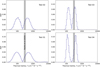 |
Fig. 2 MC model tests on asteroid Bennu. The panels show the distributions of thermal inertia solutions for different input parameters assumed to be known. The number of known parameters increases clockwise, starting from the bottom-left panel. For additional details on the test, see Table 6. The gray area in each panel marks the interval of the thermal inertia of Bennu as estimated by Rozitis et al. (2020). |
5 Estimated thermal characteristics of 2016 GE1
We performed the MC estimation of the thermal conductivity K for four fixed heat capacity values, namely C = 600,800, 1000, and 1200 Jkg−1 K−1. A random sample of one million combinations of the input parameters was used. Thermal conductivity solutions were searched for in the range between 10−8 Wm−1 K−1 and 500 Wm−1 K−1, which we believe to be more than appropriate considering the known variety of materials composing asteroids. For each K solution, we also computed the corresponding thermal inertia as
 (11)
(11)
Moreover, we ran the estimation of K with the semimajor axis drift solution given by the JPL SBDB first, and then ran it once again with the solution we obtained with OrbFit.
Figure 3 shows the distributions of K and Γ obtained for the different values of heat capacity C. Blue histograms refer to the results obtained with the JPL SBDB orbital solution, while red histograms to those obtained with our orbital fit.
All distributions have the same properties. For a thermal conductivity smaller than ~10−3 Wm−1 K−1 (thermal inertia smaller than ~100Jm−2 K−1 s−1/2), two peaks always occur with a high probability. Values for K between ~0.01 and ~1 Wm−1 K−1 and for Γ between ~100 and ~1000 Jm−2 K−1 s−1/2 are extremely unlikely. Finally, for values K ≳ 1 Wm−1 K−1 (Γ ≳ 1000 Jm−2 K−1 s−1/2), there is a low probability tail in which two more peaks occur.
The distributions are almost independent of the heat capacity C. Therefore, we always refer to the results for C = 600 J kg−1 K−1 in the following, unless explicitly stated otherwise. We performed the Kolmogorov–Smirnov test to check
whether the distributions obtained for the two solutions for the semimajor axis drift are identical. The null hypothesis was rejected with a significance level of 5%. Nevertheless, the two distributions are very similar in each of the cases shown in Fig. 3, and the results show only minor differences.
The two high probability peaks at low thermal conductivity appear at


while the corresponding peaks in thermal inertia are at


We note that these peaks are located at extremely low K, and they are almost an order of magnitude smaller than those obtained for 2011 PT (Fenucci et al. 2021, see also Fig. 9). On the other hand, the two low probability peaks at high thermal conductivity are at ~10 and ~250 Wm−1 K−1, corresponding to the thermal inertia of ~4 450 and ~18 000Jm−2 K−1 s−1/2, respectively. The presence of these two low probability peaks is due to the fact that the measured versus predicted Yarkovsky drift equation in Eq. (2) has either three or four different thermal conductivity solutions for certain combinations of input parameters. To show an example of this behavior, we computed the Yarkovsky drift on a grid in density ρ and thermal conductivity K, by fixing the other parameters to D = 9.8 m, C = 800 Jkg−1 K−1, γ = 133.77°, and P = 0.009438 h. Figure 4 shows the contour plot of the computed semimajor axis drift. The levels corresponding to the da/dt solution computed with OrbFit, together with those at 1σ uncertainty, are highlighted in red. From this figure, it can be appreciated that the measured versus predicted Yarkovsky drift equation has either three or four solutions in the interval K ∈ [10−8, 500] W m−1 K−1, for certain values of the density, ρ.
To give quantitative constraints of the thermal parameters, we fit the thermal inertia distributions by using the kernel density estimation, and then we computed the probability
 (12)
(12)
The probability P1 was always ~0.92, with negligible differences between the two solutions of the semimajor axis drift. On the other hand, the probability P2 was always ~0.08, implying that solutions with high thermal inertia are unlikely. Therefore, the results show that the thermal inertia of 2016 GE1 is probably very low, which is unexpected for the extremely fast-rotating asteroid.
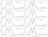 |
Fig. 3 Distributions of the thermal parameters of 2016 GE1 for different values of heat capacity, C. The first column shows the distributions of the thermal conductivity, K, and the second column the distributions of the thermal inertia, Γ. Blue histograms are the results obtained using the orbital solution provided by the JPL SBDB, while red histograms are the results obtained using our solution obtained with OrbFit. |
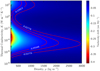 |
Fig. 4 Estimated semimajor axis drift for 2016 GE1, obtained for D = 9.8m, C = 800Jkg−1 K−1, γ = 133.77°, and P = 0.009438h. The red level curves represent the Yarkovsky drift measured from astrometry with OrbFit and the corresponding 1σ uncertainty. |
5.1 Robustness of the results
The results presented suggest that 2016 GE1 has very low thermal inertia. In this subsection we discuss how reliable such a conclusion is. The presented MC-based model for asteroid thermal inertia estimations generally depends on a set of input parameters. As demonstrated in Sect. 4, when these parameters are well known (or at least most of them), the model could provide good results for individual objects.
On the other hand, when only basic information such as orbit, absolute magnitude, and Yarkovsky drift are known, the model relies on population-based models of input parameters. In this case, the model could still provide useful results to model the thermal inertia of a population of asteroids. However, the results for an individual object are uncertain and generally unreliable. The situation with 2016 GE1 is very similar to that case, except that the rotation period is known, in addition to the orbit and absolute magnitude. This leads us to that question of why then the obtained results should be considered reliable.
The asteroid 2016 GE1 is a rapid rotator with a rotation period of only about 34 s. At the same time, a significant A2 acceleration associated with the Yarkovsky effect has been measured. A temperature gradient across the surface must be present for this effect to work. However, in the case of such a rapid rotation, the temperature gradient could exist only in the case of low thermal inertia. As a result, the rotation period strongly constrains the range of acceptable thermal inertia. In the case of 2016 GE1, only about 16% of input parameter combinations are accepted in our simulations as possible. This is largely due to solid constraints from the rotation period.
As explained in Sect. 3.2.2, despite some uncertainties, we believe the short rotation period of 2016 GE1 is determined reliably enough. Nevertheless, we tested what would happen if the rotation period is 2, 5 and 10 times longer than the measured one. In Fig. 5 we show how the resulting thermal inertia of 2016 GE1 depends on the rotation period. Increasing the rotation period shifts the distribution of thermal inertial to the right, that is to say, toward larger values. Still, even for a 10× longer rotation period, more than 90% of the solution suggests thermal inertia below 300 Jm−2 K−1 s−1/2, which can be considered low.
There are indeed small peaks in the TI distribution associated with values of Γ > \000 Jm−2 K−1 s−1/2. These values are incredibly high to the point of physical implausibility, and other studies have found very few objects with such high thermal inertia estimates (Hung et al. 2022). We, therefore, discarded them as highly improbable.
We also tested how the assumed values of the emissivity ε and the absorption coefficient α may affect the results. We found that for a reasonable range of these parameters, the changes in results are small and cannot affect general conclusions about the low thermal inertia of 2016 GE1 (see Fig. 6). Additionally, we investigated how the assumption of entirely random input distribution of the density ρ in the range 1000–3500 kg m−3 would change the result. Again, we found that the resulting thermal inertia values are not much different. Moreover, they are even shifted toward lower values (bottom panel of Fig. 6).
To conclude this part, we show how the results change when the eccentric and circular Yarkovsky models are used. As already mentioned in Sect. 3.1, the Yarkovsky model based on the assumption of a circular orbit may not be suitable due to the large eccentricity of the orbit. In Fig. 7, we show how the results differ for two Yarkovsky models when all other parameters are equal. The thermal inertia solutions in the case of the circular model favor even smaller values. Two peaks at low Γ are slightly shifted to lower values, while two smaller peaks found in the eccentric model at high values of thermal inertia disappear in the circular model. This demonstrates that the circular model is not fully suitable for NEAs that are in moderately to highly eccentric orbits. However, in the case of 2016 GE1, the results seem to be mainly driven by its rapid rotation. They, therefore, do not vary much for different input parameters or the Yarkovsky model.
With this in mind, we concluded that our estimate of the 2016 GE1 low thermal inertia is robust, even though we cannot very accurately estimate its nominal value. Nevertheless, we showed that thermal inertia of GE1 cannot exceed Γ = 300 Jm−2 K−1 s−1/2. The real thermal inertia is likely even smaller, with a probability of > 90% to be below 100 J m−2 K−1 s−1/2.
5.2 Posterior distribution of the input parameters
In addition to calculating the thermal inertia, we kept track of all combinations of input parameters for which at least a single solution of Eq. (2) was found. If no solutions are found, the measured semimajor axis drift cannot be achieved for the chosen combination, and therefore these determined values of the physical parameters are not representative for 2016 GE1.
Figure 8 shows the 2D distribution of (ρ, D) and their marginal distributions obtained for the simulations using the semimajor axis solution provided by the JPL SBDB and C = 600 J kg−1 K−1. The results in all other cases are similar. The correlations low density-large diameter and high density-small diameter are still present in the output distributions, as shown in the top panel of Fig. 8. The median value and the most likely diameter are 9.8 and 9.2 meters, respectively, which are both smaller than the values obtained for the input distribution in Fig. 1. This means that the solutions of Eq. (2) are more likely to be found for small diameters. From this distribution, we determined that 2016 GE1 has a diameter ranging from 5 m to 15 m with a probability of ~0.87 and is smaller than 20 m with a probability of ~0.94.
The density distribution peaks at about 2020 kg m−3, with a median value of ~2100kgm−3, both lower than the corresponding values of the input distribution. The probability of 2016 GE1 having a density of less than 1200 kg m−3 or more than 3000kgm−3 is small, ~0.06 in each case. We note, however, that the density distribution is two-peaked, as expected, with each peak generally corresponding to one of two main taxonomic complexes of C- and S-type asteroids. Therefore, if asteroid 2016 GE1 is found to belong to the C-type, the larger values of the density should be rejected. Additionally, if 2016 GE1 is an X-complex low-albedo but a high-density object, the assumed correlation between diameter and density would be broken, and the analysis of the posterior parameter distribution would be meaningless. We consider, however, this scenario unlikely.
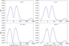 |
Fig. 5 Dependence of 2016 GE1’s thermal inertia estimation on the rotation period. The assumed period increases clockwise from the bottom-left panel. The results are shown for the nominal period solution of 34 s, as well as for 2, 5, and 10 times longer periods, as indicated in the plots. |
6 Discussion
6.1 Possible explanations for low thermal inertia
The values of Γ < 100 J m−2 K−1 s−1/2 are obtained with a probability of ~92 percent. Moreover, we have tested the stability of the result with respect to various input parameters and verified their reliability. Therefore, the results presented above strongly suggest a very low thermal inertia of the rapidly rotating asteroid 2016 GE1.
These thermal inertia values are not new for asteroids (see, e.g., Delbo’ et al. 2015). For example, the largest asteroids, such as (1) Ceres or (4) Vesta, have very low thermal inertia values of Γ < 50 Jm−2 K−1 s−1/2, as measured by Leyrat et al. (2012) and Rognini et al. (2020), and this is due to the fine regolith present at their surfaces, which in turn is made possible by the relatively high gravity of these objects.
Another cause for low thermal inertia has been recently discovered during the OSIRIS-REx and Hayabusa 2 missions, and it lies in the high micro-porosity of boulders. The ground-based estimated thermal inertia of Γ = 3\0 ± 70Jm−2 K−1 s−1/2 of Bennu (Emery et al. 2014) suggested a fine regolith-covered surface, which was not found when OSIRIS-REx arrived at the asteroid (Lauretta et al. 2019). Rozitis et al. (2020) explained the measurements with the high micro-porosity of Bennu’s surface boulders, and suggested that this could be a characteristic property of C-type asteroids. Furthermore, Cambioni et al. (2021) found that the thermal inertia of Bennu’s rocks is positively correlated with the local surface abundance of fine regolith. Similar results were obtained for Ryugu, where the global thermal inertia was estimated to be Γ = 225 ± 45 J m−2 K−1 s−1/2 (Shimaki et al. 2020), but no fine regolith-covered surface was found (Watanabe et al. 2019). In situ images taken by the Mobile Asteroid Surface Scout (MASCOT; Ho et al. 2017) lander did not detect fine regolith on the boulders. Models of the temperature variations did not fit the measurements when the regolith layer was taken into account, and the low thermal inertia was again explained by the high porosity of the boulders (Grott et al. 2019).
The spatially unresolved thermal inertia of comets is also very low, typically below 50 Jm−2 K−1 s−1/2 (e.g., Marshall et al. 2018; Groussin et al. 2019), although spatially resolved data indicate surface variations. In the case of comet 67P/Churyumov-Gerasimenko, for example, most values are in the range 10–170 J m−2 K−1 s−1/2. The thermal inertia of smooth terrains covered with deposits is lower (typically lower than 30 Jm−2 K−1 s−1/2) than those of exposed consolidated terrains (typically larger than 110 Jm−2 K−1 s−1/2) (Groussin et al. 2019).
This then raises the questions of what can explain 2016 GE1 and what the most likely scenario is. Low thermal inertia is unexpected for super-fast-rotating asteroids. On the one hand, this is because the fast rotation should clear out the surface of loose regolith. On the other hand, a large porosity often points toward a rubble-pile structure, which is also unexpected because the internal strength of such bodies might be too weak to maintain the integrity of the body under high rotational acceleration. Despite their improbability, however, none of the scenarios can be discarded, as recent models suggest that they are still possible (Sánchez & Scheeres 2020; Hu et al. 2021). The integrity of the fast rotators could be maintained by a low yield stress on the order of 25 Pa. This level of yield stress can only be explained by assuming that the particles in asteroids are small enough (on the order of a few micrometers) to form a cement matrix (glue) between the larger particles (fragments) (Persson & Biele 2021).
Still, the most likely values for the thermal inertia found for 2016 GE1 by using the semi-analytical Yarkovsky model are significantly below 100 Jm−2 K−1 s−1/2, smaller even than the thermal inertia of the boulders on Bennu and Ryugu. For the single boulder on Ryugu investigated by the MASCOT lander, Hamm et al. (2022) estimated the thermal inertia of  , corresponding to an expected porosity of
  . This means that, if 2016 GE1 was a boulder, than it would be more porous than those on Bennu or Ryugu. To get a general idea of what porosity would explain the obtained values of thermal conductivity and inertia, we applied an empirical relationship between conductivity and porosity given by Grott et al. (2019) (see also Henke et al. 2016) for meteorites. The employed empirical relation has its own limitations and, in particular, it is unreliable for large porosity. Nevertheless, it can give a first indication of the degree of porosity in 2016 GE1 needed to explain its thermal properties. We found that values of thermal inertia Γ ≤ 20 J m−2 K−1 s−1/2, compatible with two the most prominent peaks (see, e.g., Fig. 3), are only feasible for porosity ≥ 70% and density ρ ≤ 1000 kgm−3. Therefore, a highly porous, Ryugu-boulder-like object is generally consistent with our result. If so, it also means that most of the density solutions should be discarded, and only those generally compatible with C-type asteroids can be considered. This opens the possibility of small and super-fast rotators having a common origin as anomalously low-thermal-inertia boulders similar to those found on Ryugu, which may be worth exploring in the future since they are the most similar to the primordial planetesimals (Sakatani et al. 2021).
On the other hand, Sánchez & Scheeres (2020) developed a model to study under what rotational conditions an asteroid can keep thin regolith on the surface, assuming that the asteroid has a monolithic internal structure. The authors found that regolith can survive even at very small rotation periods, especially in regions at high latitudes. Given the values of low thermal inertia we found at 2016 GE1, which are the most consistent with the thermal inertia of dust-covered asteroids and the results of Sánchez & Scheeres (2020), a plausible explanation for the low thermal inertia we find at 2016 GE1 is a dust layer.
In addition to the two explanations discussed above, another cause of low thermal inertia has emerged recently, namely the cracked surface. Ishizaki et al. (2023) analyzed samples from asteroid Ryugu and found that the thermal inertia of the samples is about 3.5 times larger than the observed thermal inertia of the asteroid Ryugu’s surface. The authors suggested that this difference in thermal inertia between millimeter- and centimeter-sized returned samples and boulders could be due to the presence of large-scale cracks caused by meteor impacts (e.g., Ballouz et al. 2020) and thermal stresses (Molaro et al. 2020; Delbo et al. 2022) on a scale larger than several hundreds of micrometers in rocks and boulders on Ryugu. Therefore, the low thermal inertia of 2016 GE1 could also be due to the cracked surface.
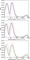 |
Fig. 6 Dependence of the resulting thermal inertia estimation on the input parameters: comparison with the nominal results. As a guide, in each plot, the results of our nominal estimation are shown as a dotted red histogram. The top panel shows the obtained thermal inertia distribution when the absorption coefficient, α, is set to 0.9 (blue histogram). The middle panel shows the results obtained assuming an emissivity, ε, of 0.9 (black histogram). The bottom panel shows how the thermal inertia distribution changes when a uniform input distribution of density, ρ, is assumed (green histogram). |
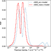 |
Fig. 7 Resulting thermal inertial distribution, Γ, with an eccentric (blue histogram) and a circular (red histogram) Yarkovsky model. In both cases, the heat capacity was set to C = 600 J kg−1 K−1. See the main text for more details. |
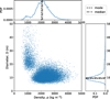 |
Fig. 8 Posterior (resulting) distribution of the parameters of GE1. The main plot shows the density, ρ, against the diameter distribution, D. The upper and right histograms show the marginal distributions of ρ and D, respectively. The results were obtained using the eccentric Yarkovsky model and a heat capacity of C = 600 J kg−1 K−1. The dashed and dash-dotted lines mark the modes and medians of the distributions, respectively. |
6.2 A population of low-thermal-inertia, super-fast-rotating asteroids?
2016 GE1 is not the only super-fast-rotating asteroid with low thermal inertia. As already mentioned, the (499998) 2011 PT shares similar thermal inertia properties, and it has a diameter of about 35 m and rotates in only 11 min. The comparative results for the two objects are shown in Fig. 9. 2016 GE1 is an extreme case of a small and super-fast rotator with extremely low thermal inertia, even lower than that found for 2011 PT. Nevertheless, the values of both objects are low and consistent with a dust-covered surface or a boulder with high micro-porosity. We note that the surface reflectivity properties of 2016 GE1 and (499998) 2011 PT are still unknown. Unfortunately, 2016 GE1 will not pass close to the Earth again in the next future, and therefore, it will not be observable due to its small size. On the contrary, 2011 PT will reach visual magnitudes smaller than 24 in June 2023, 2026, and 2029, and therefore, although still challenging, it may be observed with large-diameter telescopes. Any information in this regard would help us better understand the nature of these unusual objects and unravel their mystery.
In addition, preliminary results obtained by Petković et al. (2021) on the NEA 1998 KY26, the target of the extended Hayabusa 2 mission, showed that it might also have a relatively low thermal inertia similar to that of 2011 PT. Further, by searching for objects with a determined A2 in the JPL SBDB, many NEAs with |da/dt| > 0.007 au My−1 (a value comparable with the semimajor axis drift of 2011 PT) can be found, and most of them have an absolute magnitude H > 24. Even though information about their rotational state is not always known, the possibility that such small objects are fast rotators is still high, and therefore such a fast semimajor axis drift would still be explained by low thermal inertia. It is also important to note that these A2 measurements obtained by orbit determination are compatible with the Yarkovsky effect, except for a very small number of cases (Farnocchia et al. 2023). These facts open up the possibility for the existence of a new class of small super-fast-rotating NEAs with low thermal inertia.
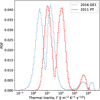 |
Fig. 9 Comparative distributions of thermal inertia for the NEAs 2016 GE1 (dotted blue line) and 2011 PT (dashed red line). In both cases, the results were obtained with the eccentric Yarkovsky model and a heat capacity of C = 600 J kg−1 K−1. |
7 Summary and conclusions
In this work we first performed a basic verification of our recently developed statistical MC method for determining asteroid thermal properties, showing that, under the particular cases of superfast rotators with large measured da/dt due to the Yarkovsky effect, we can constrain the surface thermal inertia.
We then used the model to constrain the thermal inertia of the small super-fast rotator 2016 GE1. This NEA has a diameter of less than 20 m, and its rotation period is estimated to be 34 s. We show that the thermal inertia of GE1 cannot exceed Γ = 300 J m−2 K−1 s−1/2. The real thermal inertia is likely even smaller, with a probability of >90% of being below 100 J m−2 K−1 s−1/2. The extensive testing of different input parameters confirmed the robustness of the result. Therefore, the thermal inertia was constrained to low values with a high probability.
We propose three possible interpretations for the extremely low thermal inertia of 2016 GE1: (i) a high micro-porosity; (ii) the presence of a layer of fine regolith on the surface; (iii) a cracked surface material. Therefore, this work, together with the work of Fenucci et al. (2021), not only demonstrates the usefulness of this alternative method for constraining the thermal properties of asteroid surfaces, but also opens up the possibility of the existence of a potentially new class of NEAs with super-fast rotation and low thermal inertia. Future characterizations and in situ explorations are needed to better understand the physical properties of such objects. In this context, the extended Hayabusa 2 mission will visit the small super-fast-rotating asteroid 1998 KY26 (Hirabayashi et al. 2021) and is expected to provide new insights into these very small asteroids.
Acknowledgements
We appreciate the support from the Planetary Society STEP Grant, made possible by the generosity of The Planetary Society’ members. M.F. and B.N. also acknowledge the MSCA ETN Stardust-R, Grant Agreement no. 813644 under the European Union H2020 research and innovation program.
We recall that the X-complex is degenerate in terms of albedo, containing both low- and high-albedo objects. It seems, however, to be also degenerate in terms of density, including not only asteroids of high density, but also of low density (see Fig. 5 in Berthier et al. 2023). Moreover, the low-density X-complex objects are typically those of the P-type (Usui et al. 2013), which are less likely to be present among the NEAs. Therefore, X-complex asteroids in the near-Earth region are typically those of high albedo (Thomas et al. 2011, Table 4). For these reasons, we found it reasonable to assume here that high-density X-type asteroids are also of high albedo.
References
- Alí-Lagoa, V., Müller, T. G., Kiss, C., et al. 2020, A&A, 638, A84 [EDP Sciences] [Google Scholar]
- Ballouz, R. L., Walsh, K. J., Barnouin, O. S., et al. 2020, Nature, 587, 205 [NASA ADS] [CrossRef] [Google Scholar]
- Berthier, J., Carry, B., Mahlke, M., & Normand, J. 2023, A&A, 671, A151 [NASA ADS] [CrossRef] [EDP Sciences] [Google Scholar]
- Bottke, William, F. J., Vokrouhlický, D., Rubincam, D. P., & Nesvorný, D. 2006, Annu. Rev. Earth Planet. Sci., 34, 157 [CrossRef] [Google Scholar]
- Bowell, E., Hapke, B., Domingue, D., et al. 1989, in Asteroids II, eds. R. P. Binzel, T. Gehrels, & M. S. Matthews, 524 [Google Scholar]
- Cambioni, S., Delbo, M., Poggiali, G., et al. 2021, Nature, 598, 49 [NASA ADS] [CrossRef] [Google Scholar]
- Carpino, M., Milani, A., & Chesley, S. R. 2003, Icarus, 166, 248 [NASA ADS] [CrossRef] [Google Scholar]
- Daly, M. G., Barnouin, O. S., Seabrook, J. A., et al. 2020, Sci. Adv., 6, eabd3649 [NASA ADS] [CrossRef] [Google Scholar]
- Delbo’, M., dell’Oro, A., Harris, A.W., Mottola, S., & Mueller, M. 2007, Icarus, 190, 236 [CrossRef] [Google Scholar]
- Delbo’, M., Mueller, M., Emery, J. P., Rozitis, B., & Capria, M. T. 2015, Asteroid Thermophysical Modeling (University of Arizona Press), 107 [Google Scholar]
- Delbo, M., Walsh, K. J., Matonti, C., et al. 2022, Nat. Geosci., 15, 453 [NASA ADS] [CrossRef] [Google Scholar]
- Dellagiustina, D. N., Emery, J. P., Golish, D. R., et al. 2019, Nat. Astron., 3, 341 [CrossRef] [Google Scholar]
- Del Vigna, A., Faggioli, L., Milani, A., et al. 2018, A&A, 617, A61 [NASA ADS] [CrossRef] [EDP Sciences] [Google Scholar]
- Emery, J. P., Fernández, Y. R., Kelley, M. S. P., et al. 2014, Icarus, 234, 17 [NASA ADS] [CrossRef] [Google Scholar]
- Farinella, P., Vokrouhlický, D., & Hartmann, W. K. 1998, Icarus, 132, 378 [NASA ADS] [CrossRef] [Google Scholar]
- Farnocchia, D., Chesley, S. R., Vokrouhlický, D., et al. 2013, Icarus, 224, 1 [NASA ADS] [CrossRef] [Google Scholar]
- Farnocchia, D., Chesley, S. R., Takahashi, Y., et al. 2021, Icarus, 369, 114594 [NASA ADS] [CrossRef] [Google Scholar]
- Farnocchia, D., Seligman, D. Z., Granvik, M., et al. 2023, Planet. Sci. J., 4, 29 [NASA ADS] [CrossRef] [Google Scholar]
- Fenucci, M., Novaković, B., Vokrouhlický, D., & Weryk, R. J. 2021, A&A, 647, A61 [NASA ADS] [CrossRef] [EDP Sciences] [Google Scholar]
- Flynn, G. J., Consolmagno, G. J., Brown, P., & Macke, R. J. 2018, Chem. Erde/Geochemistry, 78, 269 [NASA ADS] [Google Scholar]
- Folkner, W. M., Williams, J. G., Boggs, D. H., Park, R. S., & Kuchynka, P. 2014, Interplanet. Network Progress Report, 42-196, 1 [Google Scholar]
- Ghosal, M., Jedicke, R., & Bolin, B. 2022, in AAS/Division for Planetary Sciences Meeting Abstracts, 54, AAS/Division for Planetary Sciences Meeting Abstracts, 523.06 [NASA ADS] [Google Scholar]
- Granvik, M., Morbidelli, A., Jedicke, R., et al. 2018, Icarus, 312, 181 [CrossRef] [Google Scholar]
- Greenberg, A. H., Margot, J.-L., Verma, A. K., Taylor, P. A., & Hodge, S. E. 2020, AJ, 159, 92 [NASA ADS] [CrossRef] [Google Scholar]
- Grott, M., Knollenberg, J., Hamm, M., et al. 2019, Nat. Astron., 3, 971 [Google Scholar]
- Groussin, O., Attree, N., Brouet, Y., et al. 2019, Space Sci. Rev., 215, 29 [Google Scholar]
- Hamm, M., Grott, M., Senshu, H., et al. 2022, Nat. Commun., 13, 364 [NASA ADS] [CrossRef] [Google Scholar]
- Harris, A. W., & Drube, L. 2016, ApJ, 832, 127 [NASA ADS] [CrossRef] [Google Scholar]
- Henke, S., Gail, H.-P., & Trieloff, M. 2016, A&A, 589, A41 [NASA ADS] [CrossRef] [EDP Sciences] [Google Scholar]
- Hergenrother, C. W., Maleszewski, C. K., Nolan, M. C., et al. 2019, Nat. Commun., 10, 1291 [NASA ADS] [CrossRef] [Google Scholar]
- Hirabayashi, M., Mimasu, Y., Sakatani, N., et al. 2021, Adv. Space Res., 68, 1533 [NASA ADS] [CrossRef] [Google Scholar]
- Ho, T.-M., Baturkin, V., Grimm, C., et al. 2017, Space Sci. Rev., 208, 339 [NASA ADS] [CrossRef] [Google Scholar]
- Hu, S., Richardson, D. C., Zhang, Y., & Ji, J. 2021, MNRAS, 502, 5277 [NASA ADS] [CrossRef] [Google Scholar]
- Hung, D., Hanuš, J., Masiero, J. R., & Tholen, D. J. 2022, Planrt. Sci. J., 3, 56 [CrossRef] [Google Scholar]
- Ishizaki, T., Nagano, H., Tanaka, S., et al. 2023, Int. J. Thermophys., 44, 51 [NASA ADS] [CrossRef] [Google Scholar]
- Lauretta, D. S., Dellagiustina, D. N., Bennett, C. A., et al. 2019, Nature, 568, 55 [NASA ADS] [CrossRef] [Google Scholar]
- Leyrat, C., Barucci, A., Mueller, T., et al. 2012, A&A, 539, A154 [NASA ADS] [CrossRef] [EDP Sciences] [Google Scholar]
- MacLennan, E. M., & Emery, J. P. 2021, Planet. Sci. J, 2, 161 [NASA ADS] [CrossRef] [Google Scholar]
- Marciniak, A., Alí-Lagoa, V., Müller, T. G., et al. 2019, A&A, 625, A139 [NASA ADS] [CrossRef] [EDP Sciences] [Google Scholar]
- Marshall, D., Groussin, O., Vincent, J. B., et al. 2018, A&A, 616, A122 [NASA ADS] [CrossRef] [EDP Sciences] [Google Scholar]
- Milani, A., & Gronchi, G. F. 2009, Theory of Orbit Determination (Cambridge University Press) [CrossRef] [Google Scholar]
- Molaro, J. L., Walsh, K. J., Jawin, E. R., et al. 2020, Nat. Commun., 11, 2913 [NASA ADS] [CrossRef] [Google Scholar]
- Morbidelli, A., Delbo, M., Granvik, M., et al. 2020, Icarus, 340, 113631 [NASA ADS] [CrossRef] [Google Scholar]
- Murdoch, N., Drilleau, M., Sunday, C., et al. 2021, MNRAS, 503, 3460 [NASA ADS] [CrossRef] [Google Scholar]
- Novaković, B., Vokrouhlický, D., Spoto, F., & Nesvorný, D. 2022, Celest. Mech. Dyn. Astron., 134, 34 [NASA ADS] [CrossRef] [Google Scholar]
- Ostrowski, D., & Bryson, K. 2019, Planet. Space Sci., 165, 148 [NASA ADS] [CrossRef] [Google Scholar]
- Persson, B. N. J., & Biele, J. 2021, arXiv e-prints, [arXiv:2110.15258] [Google Scholar]
- Petković, V., Fenucci, M., & Novaković, B. 2021, in European Planetary Science Congress, EPSC2021-390 [Google Scholar]
- Piqueux, S., Vu, T. H., Bapst, J., et al. 2021, J. Geophys. Res. (Planets), 126, e07003 [NASA ADS] [Google Scholar]
- Pravec, P., & Harris, A. W. 2000, Icarus, 148, 12 [NASA ADS] [CrossRef] [Google Scholar]
- Pravec, P., & Harris, A. W. 2007, Icarus, 190, 250 [CrossRef] [Google Scholar]
- Rognini, E., Capria, M. T., Tosi, F., et al. 2020, J. Geophys. Res. (Planets), 125, e05733 [NASA ADS] [Google Scholar]
- Rozitis, B., & Green, S. F. 2011, MNRAS, 415, 2042 [NASA ADS] [CrossRef] [Google Scholar]
- Rozitis, B., & Green, S. F. 2014, A&A, 568, A43 [NASA ADS] [CrossRef] [EDP Sciences] [Google Scholar]
- Rozitis, B., Ryan, A. J., Emery, J. P., et al. 2020, Sci. Adv., 6, eabc3699 [NASA ADS] [CrossRef] [Google Scholar]
- Sakatani, N., Tanaka, S., Okada, T., et al. 2021, Nat. Astron., 5, 766 [NASA ADS] [CrossRef] [Google Scholar]
- Sánchez, P., & Scheeres, D. J. 2020, Icarus, 338, 113443 [Google Scholar]
- Shimaki, Y., Senshu, H., Sakatani, N., et al. 2020, Icarus, 348, 113835 [Google Scholar]
- Stoer, J., & Bulirsch, R. 2002, Introduction to Numerical Analysis, Texts in Applied Mathematics (Springer) [CrossRef] [Google Scholar]
- Tardioli, C., Farnocchia, D., Rozitis, B., et al. 2017, A&A, 608, A61 [NASA ADS] [CrossRef] [EDP Sciences] [Google Scholar]
- Thomas, C. A., Trilling, D. E., Emery, J. P., et al. 2011, AJ, 142, 85 [Google Scholar]
- Usui, F., Kasuga, T., Hasegawa, S., et al. 2013, ApJ, 762, 56 [Google Scholar]
- Vokrouhlický, D. 1998, A&A, 338, 353 [NASA ADS] [Google Scholar]
- Vokrouhlický, D. 1999, A&A, 344, 362 [NASA ADS] [Google Scholar]
- Vokrouhlický, D., Pravec, P., Ďurech, J., et al. 2017, AJ, 153, 270 [Google Scholar]
- Warner, B. D. 2016, Minor Planet Bull., 43, 240 [NASA ADS] [Google Scholar]
- Warner, B. D., Harris, A. W., & Pravec, P. 2009, Icarus, 202, 134 [NASA ADS] [CrossRef] [Google Scholar]
- Watanabe, S., Hirabayashi, M., Hirata, N., et al. 2019, Science, 364, 268 [NASA ADS] [Google Scholar]
- Zhang, Y., Michel, P., Richardson, D. C., et al. 2021, Icarus, 362, 114433 [CrossRef] [Google Scholar]
All Tables
Nominal osculating orbital elements of 2016 GE1 and their corresponding uncertainties at epoch 59800 MJD.
Maximum plausible range for the parameters of asteroid 2016 GE1 relevant for the magnitude of the Yarkovsky effect.
Average density and the standard deviation of the three asteroid complexes, as used in Fenucci et al. (2021).
All Figures
|
Fig. 1 Input density, ρ, versus the diameter, D, distribution for 2016 GE1. The blue histograms at the top and right show the marginal distributions of ρ and D, respectively. |
| In the text | |
|
Fig. 2 MC model tests on asteroid Bennu. The panels show the distributions of thermal inertia solutions for different input parameters assumed to be known. The number of known parameters increases clockwise, starting from the bottom-left panel. For additional details on the test, see Table 6. The gray area in each panel marks the interval of the thermal inertia of Bennu as estimated by Rozitis et al. (2020). |
| In the text | |
|
Fig. 3 Distributions of the thermal parameters of 2016 GE1 for different values of heat capacity, C. The first column shows the distributions of the thermal conductivity, K, and the second column the distributions of the thermal inertia, Γ. Blue histograms are the results obtained using the orbital solution provided by the JPL SBDB, while red histograms are the results obtained using our solution obtained with OrbFit. |
| In the text | |
|
Fig. 4 Estimated semimajor axis drift for 2016 GE1, obtained for D = 9.8m, C = 800Jkg−1 K−1, γ = 133.77°, and P = 0.009438h. The red level curves represent the Yarkovsky drift measured from astrometry with OrbFit and the corresponding 1σ uncertainty. |
| In the text | |
|
Fig. 5 Dependence of 2016 GE1’s thermal inertia estimation on the rotation period. The assumed period increases clockwise from the bottom-left panel. The results are shown for the nominal period solution of 34 s, as well as for 2, 5, and 10 times longer periods, as indicated in the plots. |
| In the text | |
|
Fig. 6 Dependence of the resulting thermal inertia estimation on the input parameters: comparison with the nominal results. As a guide, in each plot, the results of our nominal estimation are shown as a dotted red histogram. The top panel shows the obtained thermal inertia distribution when the absorption coefficient, α, is set to 0.9 (blue histogram). The middle panel shows the results obtained assuming an emissivity, ε, of 0.9 (black histogram). The bottom panel shows how the thermal inertia distribution changes when a uniform input distribution of density, ρ, is assumed (green histogram). |
| In the text | |
|
Fig. 7 Resulting thermal inertial distribution, Γ, with an eccentric (blue histogram) and a circular (red histogram) Yarkovsky model. In both cases, the heat capacity was set to C = 600 J kg−1 K−1. See the main text for more details. |
| In the text | |
|
Fig. 8 Posterior (resulting) distribution of the parameters of GE1. The main plot shows the density, ρ, against the diameter distribution, D. The upper and right histograms show the marginal distributions of ρ and D, respectively. The results were obtained using the eccentric Yarkovsky model and a heat capacity of C = 600 J kg−1 K−1. The dashed and dash-dotted lines mark the modes and medians of the distributions, respectively. |
| In the text | |
|
Fig. 9 Comparative distributions of thermal inertia for the NEAs 2016 GE1 (dotted blue line) and 2011 PT (dashed red line). In both cases, the results were obtained with the eccentric Yarkovsky model and a heat capacity of C = 600 J kg−1 K−1. |
| In the text | |
Current usage metrics show cumulative count of Article Views (full-text article views including HTML views, PDF and ePub downloads, according to the available data) and Abstracts Views on Vision4Press platform.
Data correspond to usage on the plateform after 2015. The current usage metrics is available 48-96 hours after online publication and is updated daily on week days.
Initial download of the metrics may take a while.