| Issue |
A&A
Volume 666, October 2022
|
|
|---|---|---|
| Article Number | A65 | |
| Number of page(s) | 11 | |
| Section | Celestial mechanics and astrometry | |
| DOI | https://doi.org/10.1051/0004-6361/202243049 | |
| Published online | 10 October 2022 | |
The diurnal Yarkovsky effect of irregularly shaped asteroids
1
School of Astronomy and Space Science, Nanjing University,
163 Xianlin Avenue,
Nanjing
210046, PR China
e-mail: This email address is being protected from spambots. You need JavaScript enabled to view it.
2
Key Laboratory of Modern Astronomy and Astrophysics in Ministry of Education, Nanjing University,
PR China
3
Institute of Space Astronomy and Extraterrestrial Exploration (NJU & CAST), Nanjing University,
PR China
4
State Key Laboratory for Mineral Deposits Research & Lunar and Planetary Science Institute, School of Earth Sciences and Engineering, Nanjing University,
PR China
5
Planetary Science Institute,
Tucson, AZ, USA
Received:
6
January
2022
Accepted:
22
June
2022
Abstract
The Yarkovsky effect plays an important role in the motions of small celestial bodies. Increasingly detailed observations bring the need for high-accuracy modelling of the effect. We used the multiphysics software COMSOL to model the diurnal Yarkovsky effect in three dimensions and compare the results with those derived from the widely adopted theoretical linear model. We find that the linear model shows high accuracy for spherical asteroids in most cases. We explored the range of parameters for which the relative error of the linear model is over 10%. For biaxial ellipsoidal asteroids (particularly oblate ones), the linear model systematically overestimates the transverse Yarkovsky force by ~10%. The diurnal effect on triaxial ellipsoids is periodic, and no linear model is available for this phenomenon. Our numerical calculations show that the average effects on triaxial ellipsoids are stronger than those on biaxial ellipsoids. We also investigated the diurnal effect on asteroids of real shapes and find it be overestimated by the linear model by 16% on average, with a maximum of up to 35%. To estimate the strength of the Yarkovsky effect directly from the shape, we introduced the quantity of ‘effective area’ for asteroids of any shape, and find a significant linear relationship between the Yarkovsky migration rate and the effective area. This brings great convenience to the estimation in practice.
Key words: celestial mechanics / minor planets, asteroids: general / methods: miscellaneous
© Y.-B. Xu et al. 2022
 Open Access article, published by EDP Sciences, under the terms of the Creative Commons Attribution License (https://creativecommons.org/licenses/by/4.0), which permits unrestricted use, distribution, and reproduction in any medium, provided the original work is properly cited.
This article is published in open access under the Subscribe-to-Open model. This email address is being protected from spambots. You need JavaScript enabled to view it. to support open access publication.
1 Introduction
Because of their rotation and revolution around the Sun, asteroids have an asymmetric temperature distribution on their surface, which produces asymmetric thermal re-radiation from the asteroid and thus imposes a net recoil force. This latter causes slow but continuous alteration of the asteroid’s orbit, which is referred to as the Yarkovsky effect, and is an important non-gravitational effect for metre-sized to kilometre-sized asteroids. Caused by rotation and revolution, the effect consists of two components, diurnal and seasonal effects.
Named after Ivan Osipovich Yarkovsky, a Polish engineer in Russia who, in 1901, proposed this thermal effect to compensate for the resistance of ‘ether’ (refer to Beekman 2005, 2006 for more information on Yarkovsky and the discovery of his effect), the Yarkovsky effect had been forgotten for nearly half a century, until Öpik (1951) noticed it when studying the motion of small objects orbiting the Sun. In the meantime, Radzievskii (1952) described the same effect without knowing of Yarkovsky’s work. Rubincam (1987) observationally discovered the Yarkovsky effect from the unexpected variation of the along-track acceleration of the geodetic satellite LAGEOS, and developed a ‘LAGEOS-taylored’ technique for computing the thermal force on a rapidly rotating body. Therefore, sometimes the effect is also referred to as the Yarkovsky-Radzievskii effect or Yarkovsky-Rubincam effect.
The Yarkovsky effect has become a hot topic because it has many implications for the dynamic evolution of the Solar System small bodies and the dynamics of near-Earth asteroids, including hazard mitigation for potentially hazardous asteroids (PHAs). Farinella et al. (1998) provided a unified description of the Yarkovsky effect in both diurnal and seasonal variants, and discussed some issues in meteorite science relevant to the effect. These authors proposed that small asteroid fragments in the main belt have enough mobility to reach the resonances with the help of this effect and can then be delivered to the Earth-crossing region, which provides an explanation for the fact that the meteorite cosmic ray exposure ages of near-Earth objects are much longer than their dynamical lifetimes. Farinella & Vokrouhlický (1999) calculated the semimajor axis displacements of asteroids of between 1 and 10 km in mean radius over their collisional lifetimes, and proposed that the semimajor axis drift may spread the tight clustering of an asteroid family in an observable way, a phenomenon later referred to as the V-shape in the distribution of family members.
Based on previous models (Peterson 1976; Afonso et al. 1995), Vokrouhlický (1998a, 1999) developed a complete linear model for the Yarkovsky force acting on spherical asteroids. A general formulation for both diurnal and seasonal effects was provided for any orientation of the spin axis. The main assumption is that the temperature throughout the body does not vary significantly. Vokrouhlický (1998b) also developed a similar theory for the diurnal force on spheroidal bodies. Compared with the corresponding force on a spherical body of the same mass, differences of up to a factor of three were found.
With the theoretical modelling of the Yarkovsky effect being almost complete, attention turned to its detection and its application to the motion of small objects in the inner Solar System, such as main belt asteroids, near-Earth objects, and Trojans. Chesley et al. (2003) directly detected the effect for the first time in the motion of a near-Earth asteroid, 6489 Golevka, with radar observations. Then the first detection of the effect for main belt asteroids was made by Nesvorný & Bottke (2004).
The Yarkovsky effect could be beneficial in risk mitigation concerning hazardous near-Earth asteroids (NEAs) and their potential collision with the Earth (Spitale 2002). For example, an albedo modification technique was designed as a permanently acting impact risk mitigation of a hazardous NEA (Hyland et al. 2010).
With a large number of asteroids and asteroid families, the main belt provides a good opportunity to investigate the effect. Bottke et al. (2001) demonstrated that the spreading of the Koronis family could be caused by the Yarkovsky effect instead of collisions, which resolved the contradiction that the required ejection velocities derived from collision models are much higher than results from impact experiments and simulations. Tsiganis et al. (2003) studied the 7/3 Kirkwood gap and proposed that the short-lived asteroids in it were replenished by neighbouring asteroids from the Koronis and Eos families. The Yarkovsky-aided transit of asteroids across the 7/3 gap was recently investigated in great detail by Xu et al. (2020a). Based on the V-shape spreading, Spoto et al. (2015) make a family classification and estimate their ages.
The Yarkovsky effect also plays an important role in the long-term dynamics of the Trojans of terrestrial planets. Scholl et al. (2005b) concluded that primordial Venus Trojans of tadpole orbits would have disappeared by now due to this effect. As for Mars Trojans, Scholl et al. (2005a) showed that the effect has little influence on the currently known Mars Trojans but is strong enough to destabilise Trojans smaller than 10m within 4.5 Gyr. Zhou et al. (2019) present the asymmetric stabilities of the prograde and retrograde rotating Earth Trojans due to the Yarkovsky effect and rule out the existence of undetected primordial Earth Trojans; very similarly, this happens to Venus Trojans too (Xu et al. 2022).
The improving accuracy of observations brings the need for more accurate models. Although the linear model developed by Vokrouhlický (1999) is convenient to use, its assumptions of small variation of surface temperature and circular orbits may be violated in practice. Vokrouhlický & Farinella (1998) developed a one-dimensional numerical model of the seasonal effect on large asteroids, and found that the linear approximation led to overestimation by about 15%. Spitale & Greenberg (2001) simulated the diurnal and seasonal effects on a sphere by directly solving the heat equation in three dimensions with a finite difference method. These authors found that a stony asteroid on a high-eccentricity orbit drifted in semimajor axis further than on a circular orbit. A similar numerical evaluation of the Yarkovsky effect on eccentricity was reported by Spitale & Greenberg (2002). Chesley et al. (2003) computed the Yarkovsky effect on the asteroid Golevka using a one-dimensional numerical model incorporating its radar-derived shape. Capek & Vokrouhlický (2005) proposed a complex one-dimensional numerical model, and illustrated its power using two examples, including a tumbling rotator and a binary system. Rozitis & Green (2011) developed a new complex model called the Advanced Thermo-physical Model to take account of the beaming effect caused by the surface roughness and other effects.
The benefit of the high accuracy of these numerical models is limited by their high complexity and low efficiency in computation. The linear model is still widely adopted for its simplicity. A discussion of the accuracy of the linear model was provided by Sekiya et al. (2012) for the diurnal effect on a spherical body. Based on the general solution of the temperature distribution analytically obtained from the linear model, Sekiya et al. (2012) derive the non-linear solution with an iterative method, and find that the maximum difference between the linear and non-linear solutions is 13% in terms of the rate of change of the semimajor axis. Using the multiphysics software COMSOL, Basart et al. (2012) and Groath et al. (2014) estimated the Yarkovsky effect on the asteroid 101955 Bennu (provisional designation 1999 RQ36), considering it as a spherical body, and made a simple comparison with the results from Vokrouhlický (1999) and Sekiya et al. (2012).
Considering the great convenience of the linear model of the Yarkovsky effect in application but the dearth of knowledge about its accuracy, especially for asteroids with irregular shapes, we decided to study the applicability of the linear model in greater detail. In this paper, we report our investigation of the applicability of the linear model for the diurnal effect by comparing it with the numerical model. We study two aspects in particular: the difference between the linear model and numerical simulations for spheroidal asteroids, and the deviation caused by approximating irregular asteroids as spheroids and studying them with the linear model. The rest of this paper is organised as follows. In Sect. 2, we review the basic theory of the heat transfer problem and set up our numerical model. In Sect. 3 we then compare the linear model with the numerical simulations, investigating the dependence of the validity of the linear model on the thermal, dynamical, and geometrical parameters of asteroids. Finally, we summarise our conclusions in Sect. 4.
2 Method
2.1 Basic Theory
The Yarkovsky effect is a manifestation of the non-uniform temperature distribution over the surface of an asteroid. Therefore, the core issue in modelling the Yarkovsky effect is deriving the temperature distribution in a heat transfer problem.
There are two aspects of heat transfer in an asteroid: radiation on the surface and conduction in the interior. In a rotating body-fixed frame, heat conduction can be described by the Fourier equation of temperature T:
 (1)
(1)
where ∇2 is the Laplace operator, and K, C, and ρ are the thermal conductivity, specific heat capacity, and density of the material, respectively. The radiation happens on the asteroid’s surface, which leads to a boundary condition reflecting the conservation of energy:
 (2)
(2)
The first terms on the left-hand side and the right-hand side are radiation terms accounting for the energy re-radiated by the asteroid to outer space and the energy absorbed from the Sun, respectively. The second term accounts for the energy conducted to the deeper layers of the asteroid. Here, ϵ denotes the emissivity, σ the Stefan-Boltzmann constant, n the unit vector normal to the surface, α the absorption coefficient, and ℰ the external (solar) radiation flux. These two equations are difficult to solve analytically and some approximations must be made, such as the linear approximation proposed by Vokrouhlický (1998a).
As long as the temperature distribution is derived somehow, and assuming a Lambert surface, the net recoil force of the thermal radiation of the asteroid can be obtained:
 (3)
(3)
where c is the speed of light, S is the unit surface area, and the integral domain is the whole surface.
2.2 Numerical Setup
The temperature distribution in our model is numerically simulated using the commercial software, COMSOL Multiphysics®1, which is designed to solve complex physical problems involving coupled physical processes with a high degree of freedom. Unlike in most 1D numerical models, the interactions between surface elements, including surface-to-surface shading and radiation, are considered in our simulations.
The model is set in three dimensions (3D). The heat transfer, inside the body by conduction and on the surface by radiation, is calculated taking into account the surface-to-surface radiation. A temporal (non-stationary) distribution of surface temperature in the rotating body-fixed frame is calculated using COMSOL.
Assuming the asteroid is a perfect sphere, we create a sphere of radius R = 1 m and set its physical parameters. For simplicity, the thermal conductivity K and specific heat capacity C are set as constants, and the emissivity is equal to the absorption coefficient, ϵ = α = 0.9. Initially the asteroid is assumed to be an isothermal sphere, with its initial temperature being determined by the equilibrium between its thermal radiation and absorption from the solar radiation, that is 4πR2 · ϵσT4 = πR2 · αℰ.
The heat flux ℰ depends on the distance between the asteroid and the Sun. In a rotating body-fixed frame, the Sun orbits the asteroid, acting as an external radiation source. The orbital period of the Sun is the rotation period of the asteroid P.
Observing from an inertial (non-rotating) frame, we are supposed to see a static temperature distribution in the asteroid. When the temperature variation at the subsolar point on the surface of the asteroid is less than 1% in a rotation period, we regard the equilibrium as being reached, which generally takes an integration time of 50 P in most cases of our simulations.
One of the critical steps in the numerical scheme of the finite element method (as in COMSOL) is to build the mesh. An appropriate mesh must be a compromise between accuracy and efficiency. After many tests of the spherical asteroid model, we generate a mesh of prisms to fill the spherical shell and fill the central cavity with tetrahedral mesh. The core of the sphere has little effect on the final temperature on the surface, because the heat flux cannot penetrate deeply in most cases when the object is above a certain size, thermal inertia is below a certain threshold, and rotation is above a certain speed. Therefore, in practice, a hollow sphere – instead of a solid one – is accurate enough to model the asteroid if a boundary condition of thermal insulation is set on the inner surface of the spherical shell with an appropriate thickness.
2.3 Mesh Building
The heat transfer and temperature variation in an asteroid occur mainly on the surface and in the shallow subsurface region, but not deep below the surface of the body. We show this by calculating the temperature in the body of an asteroid of 1 m in radius as an example. We parametrise the asteroid like a typical regolith-covered asteroid with a density ρ = 1500 kg m−3, a conductivity K = 0.0015 W m−1 K−1, and a specific heat capacity C = 680 J kg−1 K−1. A rotation period P = 1000 s, a spin axis obliquity γ = 0°, and a heliocentric distance r = 1 AU are also assigned. These parameters are adopted in the rest of the paper unless specifying otherwise. We realise that the period of 1000s is very short, even for a small asteroid of 1 m radius, but this value does not affect the following analyses in this paper and in fact the value P can be traded with ρ or C, as we show below.
As illustrated in Fig. 1, along the depth direction, the temperature at each point varies with time as the asteroid rotates and the heat propagates inside. For a point on the asteroid surface (depth 0.0 mm), the temperature is high near local noon (when it is the subsolar point), and as the asteroid rotates, the temperature drops down through dusk, midnight, and dawn. It is worth noting that the hottest moment generally is not at noon but shortly after noon due to the ‘thermal inertia’ of the asteroid material. For the same reason, on a subsurface point, for example at a depth of 0.7 mm, the temperature around dusk is higher than at noon. Going deeper inside, the temperature approaches a constant value; that is, below a certain depth the asteroid core has a static temperature. In practice, for the purpose of studying the thermodynamics, we can simulate the asteroid by a spherical shell of a certain thickness and a solid core of a constant temperature, as we mentioned above in Sect. 2.2.
As heat transfer and temperature variation happen mainly in the skin layer of the asteroid, the thickness of that layer could be a good reference for our mesh-building strategy. There is a characteristic quantity called ‘penetration depth’ in the literature that can be derived by dimensional analysis, and is defined as (Wesselink 1948)
 (4)
(4)
Taking the parameters assigned to the asteroid adopted in this paper, the penetration depth can be calculated as ls ≈ 0.5 mm. At this depth, the fluctuation of temperature decreases to 1/e of the surface amplitude. Theoretically, at a depth of nine times ls, the variation reduces to 1/e9 ≈ 10−4.
To determine a practical thickness of the hollow shell, we performed a couple of tests. In these tests, we tried different thicknesses of the shell and calculated the temperature on the surface with which the Yarkovsky force can be obtained through Eq. (3). As the force component in the transverse direction (perpendicular to the incident solar radiation in the orbital plane) dominates the Yarkovsky effect on semimajor axis drifting, we show the temperature profile along the equator and the transverse Yarkovsky force Ft in our tests in Fig. 2.
As shown in Fig. 2, the adopted thickness of the presumed shell influences the results significantly. The temperature profile of the case with a shell thickness of 0.5 mm (= ls) is apparently different from that with a thickness of 5.0 mm (upper panel), which results in a significant difference (about 70% relatively) in terms of the transverse Yarkovsky force (lower panel). The calculated force varies significantly when a small thickness is adopted, and gradually converges to a certain value when the thickness increases. The variation is clearly an artificial effect due to the fact that the adopted shell is too thin to practically embody the thermodynamic cycle of the surface layer within. We find in the lower panel of Fig. 2 that the deviation of Ft from the convergent value (1.04497 µN) at a thickness of 2.5 mm is about 0.1% and reaches ~10−5 at 4.0 mm. In this paper, we therefore conservatively set the thickness of the hollow shell to ten times the penetration depth (10ls), although we suggest 5ls for general purposes. Hereafter, our numerical model of an asteroid is assumed to consist of a shell of 10ls in thickness and an isothermal core the temperature of which is the same as at the inner boundary of the shell. Such a mesh strategy leads to tens of thousands of mesh elements, and our desktop workstation computer takes typically one hour to compute each simulation up to the point at which a steady temperature distribution is reached.
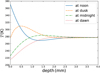 |
Fig. 1 Temperature along a certain radius on the equatorial plane at four different times. The depth is measured downwards from the surface. |
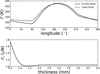 |
Fig. 2 Influence of adopted shell thickness on the simulated results. Upper panel: temperature distribution along the equator for two values of shell thickness. Lower panel: dependence of the simulated transverse Yarkovsky force on the adopted shell thickness. |
3 Comparisons with Linear Models
It is difficult to analytically obtain the temperature distribution on the surface of an asteroid from Eqs. (1) and (2). However, in the linear model, a solution was found when assuming that the temperature does not vary greatly throughout the asteroid’s surface, meaning that the term T4 in Eq. (2) could be linearised via Taylor expansion. However, in the example shown in Fig. 1, the temperature varies between a minimum of 215 K and a maximum of 370 K, that is, more than 70% higher. In addition, even if the linear model is used, the equations can only be solved analytically for asteroids with certain specific regular shapes.
Therefore, pure numerical simulations are still necessary in many circumstances. Meanwhile, the linear model provides an appropriate estimation of the Yarkovsky effect when the shape of the asteroid is unknown. It is worth assessing the deviation of the linear model from the numerical simulations for asteroids with different shapes, which is the purpose of this paper. We present our investigations of the Yarkovsky effect for spherical, ellipsoidal, and irregular asteroids.
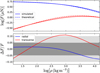 |
Fig. 3 Comparisons of the Yarkovsky forces derived from the linear model (theoretical) and numerical simulations for varying density ρ. Upper panel: forces (blue for radial and red for transverse components) versus ρ. Solid curves refer to simulated results while dashed curves are for the linear model. Lower panel: fractional differences between the results from two methods. Blue and red curves are for the radial and transverse components, while grey and light-grey areas indicate the difference of less than 5 and 10%, respectively. |
3.1 Spherical Asteroid
Assuming a spherical asteroid of radius R = 1.0 m on a circular orbit at a distance of r = 1.0 AU from the Sun, and using the numerical simulation (via COMSOL) and the linear model (Vokrouhlický 1998a), we calculate the Yarkovsky effect fordifferent values of parameters. By these calculations, we can check the dependence of the Yarkovsky effect on parameters, and verify the validity of the linear model under different conditions. For this purpose, we calculate the Yarkovsky force or the rate of semimajor axis migration.
As mentioned in Sect. 2.3, the heat conduction is limited in a thin layer (we adopt 10ls in this paper). The temperature distribution on the surface of an asteroid (and therefore the accuracy of the linear model) is generally independent of its size, unless the penetration depth is comparable to this latter. We therefore note that the radius of R = 1.0 m adopted here is large enough to show the relative accuracies of the linear theory.
3.1.1 Dependence on ρ, C, and P
Figure 3 shows our calculations with density ρ as the variable. To obtain the results in this figure, all parameters but ρ are fixed (C = 680J kg−1 K−1, K = 0.0015W m−1 K−1, P = 1000s as mentioned before). The heat transfer is slower – and the hottest spot on the asteroid surface is further from the subsolar point – when the material density is higher. As a result, the transverse component of the Yarkovsky force, which is the net recoil force of the thermal radiation, will increase as ρ increases, while the radial component decreases for the same reason, just as we can see from Fig. 3. In the meantime, the peak temperature decreases with increasing ρ, and this is why the transverse force begins to decrease when log ρ > 3.5.
A similar argument can be made for the parameter of specific capacity C. If we regard the rotation period P as a parameter and measure time in P, that is, substitute time t by τ = t/P, then Eq. (1) can be rewritten as
 (5)
(5)
We note that ρ, C, and P appear only here in equations describing the thermal dynamics. Consequently, these three parameters degenerate into a combination (ρC/P), and thus the Yarkovsky effect depends on C and 1/P in a similar way to its dependence on ρ (Fig. 3). This is also confirmed by our numerical simulations.
The differences between the results from numerical simulations and the linear model can be seen in Fig. 3, particularly in the transverse component of the force that drives the asteroid to drift in semimajor axis. It must be noted that the differences are acceptable. The relative difference shown in the lower panel of Fig. 3 is nearly always within 10%, implying that the linear model works very well in most cases for spherical asteroids.
We note that the relative difference for transverse force is a little above 10% for the density around ~103 kg m−3. Taking the fixed parameters C and P adopted in calculations, this corresponds to ρC/P ~ 680 J K−1 m−3 s−1. In addition, at around log ρ = 1.7, corresponding to ρC/P ~ 35 J K−1 m−3 s−1, the relative deviations of both radial and transverse forces are very close to zero simultaneously. If we fix ρ = 1500 kg m−3 and C = 680 J kg−1 K−1, these two ρC/P values can be translated to rotation periods of 1500 s and 30 000 s, respectively.
3.1.2 Dependence on K
Different from ρ, C, and P, the thermal conductivity K is involved in both Eqs. (1) and (2), which might make the dependence on it more complicated. Meanwhile, being difficult to measure directly in astronomical observations, the K of an asteroid is generally of high uncertainty. We carried out similar calculations for varying K as we did for ρ, and summarise the results in Fig. 4. In general, a large value of conductivity K is conducive to the heat transfer inside an asteroid, meaning that the temperature on its surface tends to reach a uniform distribution quickly, leading to a small Yarkovsky effect, which is reflected by the overall descending profile of curves in the upper panel of Fig. 4.
To describe the relaxation of surface temperature with respect to rotation, Farinella et al. (1998) introduced a parameter Θ, which is defined as the ratio between the infrared energy radiated away from the surface in a rotational period  and the thermal energy stored in the ‘thermally affected surface shell’
  :
:
 (6)
(6)
where  denotes the average temperature in the thermally affected surface shell with a thickness of δ, which can be roughly estimated as the penetration depth δ = ls. According to the definition, Θ > 1 indicates that energy would be stored in the surface layer efficiently while the temperature gradients on the surface would be built up inefficiently, resulting in a small Yarkovsky effect, and vice versa.
Three regimes can be seen in the upper panel of Fig. 4. From left to right, in the first regime of small K, the radial component of the Yarkovsky force is higher than the transverse component, implying that the radiation delay angle (the angle between the hottest spot and the subsolar point) increases with K but is always beneath 45°. This regime is expected to be separated by Θ = 1 (where δ = ls(K)) from the second regime where the radial Yarkovsky force is almost the same as the transverse force.
In the second regime, the transverse Yarkovsky force being approximately equal to the radial force implies a radiation delay angle of almost 45°. This regime ends when the thickness (δ) of the thermally affected layer is equal to the asteroid radius. Obviously, the thickness δ increases with K, and therefore for a given radius R the condition δ = R is met at a certain value of K. We plot the location of δ = ls = R in Fig. 4. It is worth noting that two lines of Θ = 1 and ls = R serve as the boundaries of three regimes fairly well.
In the third regime, where ls > R, the radial force deviates from the transverse force, that is, the delay angle begins to decrease from 45°. When an asteroid is so small (or equivalently, the conductivity is so large) that the heat may transfer easily across the body from one side to the opposite side, the temperature gradients (even between the day and night sides) will fail to appear and the Yarkovsky effect begins to vanish quickly.
As shown in the lower panel of Fig. 4, the relative difference between the numerical simulation and linear model is always within 10%, and it converges to zero with increasing K. For large thermal conductivity, the energy from solar radiation can be quickly conducted to other regions, and the variation of temperature across the asteroid will be small, so that the condition for the linear model is very well satisfied. However, the difference does not vanish monotonically with increasing K because the Yarkovsky force depends not only on the temperature asymmetry on the surface but also on the average temperature.
Substitution of the thickness δ in Eq. (6) by the penetration depth in Eq. (4) leads to  . We note that ρ, C, and K in the numerator are all parameters of the material. Indeed, the numerator is simply the ‘thermal inertia’
 (7)
(7)
which represents the capacity of a material to store heat and to delay its transmission (Ferrari 2007). Γ = 0 indicates instantaneous equilibrium with solar radiation throughout the surface, while Γ = ∞ implies a surface with a constant temperature (Spencer et al. 1989).
The thermal inertia plays an important role in geophysics and planetary science. It is the prime intermediary between remote temperature observations and the geological information including the particle size, rock abundance, bedrock outcropping, and the degree of induration (Palluconi & Kieffer 1981; Wang et al. 2010), which in turn determine the Yarkovsky effect. In general, the thermal inertia is supposed to dictate the strength of the Yarkovsky effect (Delbo et al. 2015). However, results deduced from the linear model show that this is only true for the asteroids of large size (Xu et al. 2020b). Here, we verify the statement with numerical simulations.
For a typical regolith-covered asteroid, ρ = 1500 kg m−3, C = 680J kg−1 K−1, K = 0.0015 W m−1 K−1, and therefore the thermal inertia Γ0 = 39.11 J m−2 K−1 s−1/2. Keeping this Γ0 constant, we vary K and ρC according to  , and run numerical simulations of the Yarkovsky effect. In addition, from the definition of penetration depth, we have
  , and therefore a varying K (but fixed Γ) can be translated to a varying R/ls, where R is the fixed radius of the asteroid (1.0 m here). We show the transverse Yarkovsky force of an asteroid with constant thermal inertia (Γ0) but varying K in Fig. 5.
For asteroids of large size (R ≫ ls), the Yarkovsky force remains constant, implying that it is determined (solely) by the thermal inertia Γ. However, for small asteroids whose sizes are comparable to or smaller than the penetration depth, the force varies even when the same Γ value is kept, implying that Γ alone does not determine the strength of the Yarkovsky effect. In fact, the solution in which the heat transfer depends on Γ alone can only be obtained when an adiabatic boundary condition is fulfilled (Spencer et al. 1989), that is, a deep layer of constant temperature exists. When the asteroid is so small – or equivalently the thermal conductivity K is so large – that its radius is comparable to the penetration depth, which in practice is rare, the Yarkovsky effect cannot be correctly estimated if only the thermal inertia is known.
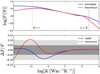 |
Fig. 4 Same as Fig. 3 but for varying thermal conductivity K. In the upper panel, the vertical orange dotted line refers to the location of Θ = 1 while the vertical grey dashed line indicates where the penetration depth is equal to the radius of the asteroid. |
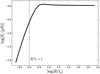 |
Fig. 5 Transverse Yarkovsky force of asteroids with given Γ but different sets of ρ, C, and K (see text). The dotted line refers to R/ls = 1. |
3.1.3 Dependence on r
As the original driver of the Yarkovsky force – the solar radiation flux – is inversely proportional to the square of heliocentric distance r, the Yarkovsky effect changes with respect to r. Fixing other parameters at typical values but varying the heliocentric distance, we carry out similar calculations and make comparisons as in the previous subsections and summarise the results in Fig. 6.
The Yarkovsky effect declines quickly as the heliocentric distance r increases. Further away from the Sun, the equilibrium temperature on an asteroid decreases, and thus the thermal parameter Θ in Eq. (6) increases. The upper panel of Fig. 6 can be divided into two regimes. In the left regime of small r and Θ < 1, the transverse force is smaller than the radial force. To the right of Θ = 1, the Yarkovsky effect is relatively weak but the radial and transverse forces are almost equal to each other.
The lower panel of Fig. 6 shows that the relative difference of the forces obtained from numerical simulations and derived from the linear model is within 10% in most cases and converges to null when r increases. However, the consistency is broken when the asteroid is close to the Sun, with the difference between the transverse forces derived from two methods reaching 20% at r = 0.1 AU. Therefore, particular attention should be paid if we apply the linear model to asteroids on orbit close to the Sun, or equivalently if the central star has a high luminosity.
3.2 Biaxial Ellipsoid
Vokrouhlický (1998b) also developed a linear model for biaxial ellipsoids rotating around the axis of symmetry. They considered a class of biaxial ellipsoids with different equatorial radii R and polar radii e1R, and compared their Yarkovsky forces with those of spherical bodies with the same volume.
Keeping the physical and dynamical parameters the same as the ones adopted for the spherical asteroid model in the previous subsection, we carry out several calculations of the Yarkovsky effect for ellipsoids with the same volume as that of a spherical asteroid of radius 1.0 m but with oblateness e1 ranging from 0.3 to 3.0. The results are summarised in Fig. 7. We note that the rotation around the polar axis for ellipsoids with e1 > 1 is unstable and thus rare in reality. We ignore the stability problem because our main concern in this paper is the calculation of the Yarkovsky effect.
In Fig. 7, the Yarkovsky forces acting on a biaxial ellipsoid and a sphere of the same volume are denoted by F1 and F0, respectively. The ratio F1/F0, both for the radial and transverse components, increases from ~0.5 to ~1.75 when e1 increases. For oblate ellipsoids (e1 < 1), the Yarkovsky forces are smaller because the normal vectors of facets on the surface are more likely to be aligned with the spin axis. On the contrary, the forces are relatively large for prolate ellipsoids (e1 > 1).
The lower panel of Fig. 7 shows the relative differences between the results for biaxial ellipsoids derived by the linear model and numerical simulations. Although in most cases the deviation (∆F1) of the linear model from the numerical simulation (F1) is within 10% (for transverse force) or even 5% (for radial force), it should be noted that the transverse force derived from the linear model is always larger than the numerical results (∆F1 > 0), implying that a slight but systematic overestimation exists in the linear model for the semimajor axis drift driven by the Yarkovsky effect. We also note that, for oblate ellipsoids, the difference goes up with decreasing oblateness parameter e1, and it is worse for the radial force (up to ~20% when e1 → 0.3). In fact, the temperature variation around the equatorial area is relatively large for oblate ellipsoids, meaning that the linear approximation causes a greater deviation for the oblate ellipsoids than for prolate ellipsoids.
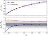 |
Fig. 7 Yarkovsky forces acting on biaxial ellipsoids and the difference between the linear model and numerical simulations. Upper panel: ratio of the forces acting on ellipsoids F1 to those on the sphere F0 versus oblateness e1. Lower panel: relative differences between the forces derived from the linear model and numerical simulations. Blue and red mark the radial and transverse components, respectively. |
3.3 Triaxial Ellipsoid
Releasing the assumption of having an axis of symmetry from the biaxial ellipsoid model, we have a triaxial ellipsoid that could serve as a better approximation of many asteroids, and there is no longer a linear model of the Yarkovsky effect available for this case. The ellipsoids considered here have the same volume as a sphere of radius 1.0 m, and they are characterised by three free semi-axes (aX, aY, aZ). Two parameters e1, e2 describing the shape are defined as:
 (8)
(8)
When e2 = 1, a triaxial ellipsoid reduces to a biaxial ellipsoid, and we note that ellipsoids characterised by parameter e2 and 1 / e2 are the same in shape.
Without the rotational symmetry, the temperature distribution on the surface of a triaxial ellipsoid in the non-rotating frame should be periodic rather than static, and therefore the Yarkovsky force most probably is not constant, as the example in Fig. 8 shows. Both the radial and transverse forces oscillate with a period of half of the rotation period. Furthermore, we find that the oscillation amplitudes will be amplified if e2 increases. During the oscillation, the transverse force may even change direction (from positive to negative, or vice versa).
Being the net recoil force of the thermal radiation, the Yarkovsky force generally points in the opposite direction to the surface normal direction at the hottest spot. Thus, the angle θ between the radial-in vector (pointing from the subsolar point to the Sun) and the surface normal vector at the hottest spot determines the direction of the Yarkovsky force. Obviously, for a prograde (retrograde) spherical asteroid, θ > 0 (θ < 0) and the transverse Yarkovsky force is positive (negative). However, for a prograde-rotating (around Z-axis) triaxial ellipsoid, when the long axis (X-axis for e2 > 1) passes over the subsolar point, we may have θ < 0 for a while, of which the duration depends on e2 and thermal parameters. This is a simple explanation of why the curve of transverse Yarkovsky force periodically crosses F = 0 in Fig. 8.
The oscillating force can be averaged over one rotation period. To compare the Yarkovsky effect on a triaxial ellipsoid to that on a biaxial ellipsoid, we calculate the time-averaged forces (denoted by F2) for several triaxial ellipsoids, of which the volume, e1, and thermal parameters are the same as those for the corresponding biaxial ellipsoids. We denote the forces on the biaxial ellipsoids by F1 and plot the ratio F2/F1 in Fig. 9.
The results show that larger Yarkovsky forces are produced on triaxial ellipsoids than on biaxial ellipsoids, and the smaller the e1, the larger the difference. For a given e1, the ratio F2/F1 increases as e2 increases. Particularly for prolate ellipsoids (e1 > 1), the Yarkovsky force on the triaxial ellipsoid is larger than the one on the biaxial ellipsoid (F2 > F1), while the latter is larger than the force on a sphere of the same volume (F1 > F0, see Fig. 7). Consequently, the Yarkovsky effect on prolate ellipsoids is significantly stronger compared to the spherical asteroids. If we adopt the linear model for spheres or for biaxial ellipsoids to calculate the Yarkovsky effect on a triaxialellipsoid-like asteroid, the estimation may have an error of up to ~40% (Fig. 9), depending on how much the shape deviates from a sphere or a biaxial ellipsoid.
Another interesting inference from the above calculations refers to the evolution of binary asteroids. Consider a pair of asteroids that are similar in size, rotation, and composition. If their shapes are different from each other, they might suffer significantly different Yarkovsky effects, resulting in the disassembly of the binary. Therefore, we are likely to see that the pair of asteroids in a binary are similar to each other in shape.
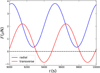 |
Fig. 8 Evolutions of the radial force (blue) and transverse force (red) acting on a triaxial ellipsoid in one rotation period. The flattening parameters e1 = 0.3 and e2 = 3. |
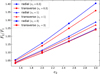 |
Fig. 9 Ratio of the forces acting on triaxial ellipsoids F2 to those on biaxial ellipsoids of the same volume F1 versus the flattening parameters e1 and e2. Blue and red are for radial and transverse forces, while solid circles, triangles, and squares refer to e1 = 0.3, 1, and 3, respectively. |
3.4 Real Asteroids
Although a growing number of observations indicate that asteroids are generally of irregular shapes even if small-scale structures are ignored, it is common to estimate the diurnal Yarkovsky effect by assuming the asteroid is an equal-volume sphere and thus using the linear model. On the one hand, small asteroids, which are usually the most affected by the Yarkovsky effect, are more likely to have irregular shapes, because their self-gravity is too weak to modify them towards symmetrical shapes unless other effects such as rotational deformation are acting on them. On the other hand, the linear model introduces some errors even for regular shapes like spheres or biaxial ellipsoids, as we show above. Instead of creating more fictitious shapes, here we use a sample of real asteroid shapes to check the difference between the approximation of the linear model and numerical simulations.
The shapes of 34 real asteroids adopted here are downloaded from the Planetary Data System2, and we show 4 of them in Fig. 10. To facilitate the comparison, all asteroids are scaled to have the same volume as a 10m-radius sphere, and are assumed to have the same thermal parameters ρ, C, and K as for the models described previously. All but one (4179 Toutatis, see Fig. 10) of them are assumed to rotate around the principal axis of the maximum moment of inertia with a period of 30 min (1800 s), and they are put on circular orbits at 1 AU from the Sun. We emphasise here that these 34 asteroids provide us nothing but a sample of diverse shapes. We note that the arbitrarily selected rotation period (30 min) here is short and not common, but the purpose of this paper is not to give the Yarkovsky effect for a specific asteroid, and in addition, as we mentioned previously in Sect. 2.3, the period can be traded with the density ρ and heat capacity C. Moreover, the dependence of the Yarkovsky effect on rotational period is already known (see e.g. Xu et al. 2020b).
For the sake of making direct comparisons, we calculate the rate of semimajor axis drift (da/dt) instead of the surface temperature or the Yarkovsky forces, simply because the semimajor axis drift is the most prominent manifestation of the diurnal Yarkovsky effect. We calculate the da/dt using a semi-analytical method as follows.
In the study of the diurnal Yarkovksy effect, as the rotation period is much shorter than the orbital period (1 yr), it is reasonable to assume that the temperature distribution on the surface of the asteroid has reached an (dynamical) equilibrium state at any phase of its orbit. Therefore, it is possible to calculate the surface temperature and average the Yarkovksy force over one rotational period on each position along the orbit. Substituting the Yarkovsky force – now described by a function of the orbital phase (true anomaly) – into the Gaussian planetary equations and averaging over one revolution, we obtain the rate of semimajor axis drift da/dt.
We summarise our calculations in Fig. 11, in which the obliquity of spin axis γ of each asteroid is tested in the range from 0° to 180°. In the linear model for a spherical asteroid, da/dt ∝ cos γ, just as the dashed curve in Fig. 11 shows, and it seems that this relation holds for asteroids of arbitrary shapes. For all asteroids in the sample, the diurnal Yarkovsky effect drives the prograde-spinning asteroids (γ < 90°) to migrate outward (da/dt > 0) and the retrograde rotators (γ > 90°) inward (da/dt < 0). The dependence of migration direction on obliquity is not affected by the shape.
However, the drift rate |dα/dt| is moderately affected. Except for two ‘outliers’ corresponding to Toutatis-like and Kleopatralike asteroids (see Fig. 10), the remaining 32 asteroids of real shapes migrate at a slower pace than that analytically derived from the linear model for spherical asteroids (dashed curve in Fig. 11). At γ = 0°, the linear model gives da/dt = 0.0217 AU Myr−1, while the numerical results of the 32 asteroids are distributed from 0.0160 AU Myr−1 to 0.0212 AU Myr−1, with an average value of 0.0187 AU Myr−1. Such statistical results reveal a possible error in the linear model. If we adopt the linear model for spherical asteroids to calculate the semimajor axis drift of asteroids with these real shapes, we overestimate da/dt by 16% on average, while the maximum deviation can reach 35%.
The slowest Yarkovsky migration (0.0160 AU Myr−1) is shown by a Nereus-like asteroid, and the second slowest is a Steins-like asteroid, both shown in Fig. 10. Compared to other asteroids, these latter two are apparently more oblate. On an oblate asteroid, the normal directions of surface elements have relatively small components parallel to the equatorial plane, and therefore the recoil force of the thermal radiation (always in the normal direction) is relatively small and the migration is relatively slow. On the contrary, if the normal direction of surface elements tends to be parallel to the equatorial plane, a relatively high migration speed will be expected. We note that the two ‘outliers’ of faster migration in Fig. 11 are the Toutatis-like asteroid (da/dt = 0.0287 AU Myr−1) and the Kleopatra-like asteroid (da/dt = 0.0229 AU Myr−1). These latter do have more surface elements facing outwards in directions parallel to the equatorial plane (see Fig. 10). Particularly, in our calculations, 4179 Toutatis is simply assumed to rotate around its long axis, although it is in fact in a complex rotation state (see e.g. Zhao et al. 2015).
In fact, an index of shape can be defined as follows, which can be used to directly decipher the strength of the Yarkovsky effect in driving the semimajor axis drift. The shape of an asteroid can be described by a set of surface elements with different sizes dS and orientations n, while the combination of (dS, n) determines the capability of thermal re-radiation in a certain direction, which is equivalent to the strength of the Yarkovsky effect.
As the penetration depth is very small compared to the radius of the object with thermal parameters adopted in this paper (~0.5 mm), the lateral heat transfer can be ignored and the heat transfer in a rotational period must be strongly localised. In a certain surface element, the thermodynamic process of absorption, storage, and re-radiation of energy should occur mainly inside the same surface element. As a result, the Yarkovsky effect, arising from the recoil force of re-radiation, is determined by the energy budget and the orientation of each individual surface element. The overall Yarkovsky effect of an asteroid is the integration of these surface elements across the whole surface. Furthermore, if we focus on the influence of shape on the Yarkovsky effect, we can use this integration as an index, and a comparison to the index of a standard model (e.g. a sphere) will directly give the relative strength of the Yarkovsky effect.
Consider a surface element dS of area dS at its local noon, when the Sun is on the plane spanned by its normal vector n and the Z-axis (spinning axis). We note that these vectors are defined in an asteroid-centred inertial frame. The dS absorbs the solar radiation with a flux (power) Ein:
 (9)
(9)
where nin is the direction of incident radiation, lying in the equatorial plane (XY plane) when γ = 0. All the absorbed energy will be re-radiated out from the same area (localisation assumption) after a delay, which, depending on thermal inertia Γ, is constant for each surface element. Correspondingly, the strongest recoil force of the re-radiation will be acting in the reverse normal direction (−n) when dS reaches the peak temperature, and the deviation from the local meridian normal direction is determined by the thermal delay and the object’s rotation period P. In addition, considering the fact that the thermal evolution of a surface element during a rotational period is (approximately) symmetric with respect to the peak temperature position, a simple calculation reveals that the overall recoil force produced by this surface element during a rotational period is proportional to the recoil force at the moment when it is experiencing the peak temperature.
As all surface elements have the same Γ and P, a constant delay between the absorption and re-radiation of energy for each surface element indicates that the projection of the overall recoil force of each surface element over a rotational period on the XY plane points in the same direction. An integration of all these surface elements across the whole surface of an object leads to the overall Yarkovsky force, the projection of which on the XY plane certainly points in the same direction. Therefore, when we discuss the relative strength of the Yarkovsky effect among asteroids with the same Γ and P, we know that they all have the same delay in direction and the specific value of delay does not matter. Without loss of generality, the delay is assumed to be null, that is, the re-radiation is assumed to happen simultaneously with the absorption in the direction n at noon.
In this paper, we investigate the semimajor axis migration due to the Yarkovsky effect, and therefore only the force component in the orbital plane (coinciding with the equatorial XY plane when γ = 0°) is of interest. Finally, for null delay, the reradiation power from dS that produces the recoil force on the orbital plane is
![Mathematical equation: ${E_{{\rm{out}}}} \propto \left[ {{\bf{n}} \cdot \left( { - {{\bf{n}}_{{\rm{in}}}}} \right)} \right]{E_{{\rm{in}}}} \propto {\left( {{\bf{n}} \cdot {{\bf{n}}_{{\rm{in}}}}} \right)^2}{\rm{d}}S.$](/articles/aa/full_html/2022/10/aa43049-22/aa43049-22-eq16.png) (10)
(10)
The total effect can be obtained by integrating (n · nin)2dS over the whole surface of an object. We note that this integration should be done by rotating the object in the asteroid-centred inertial frame, and the result is an ‘effective area’. As a ‘standard shape’, the effective area of a sphere with radius R is 8πR2/3.
The effective area tells us the capability of an object to produce the recoil force by re-radiation, and can therefore serve as the index of the relative strength of the Yarkovsky effects acting on asteroids of different shape but with the same thermal parameters. Again, using the 34 real asteroids (all scaled to have the volume of a 10 m-radius sphere) as examples, we calculate their effective areas, and Fig. 12 shows the relation between the da/dt of these asteroids with obliquity γ = 0° and their effective areas. The da/dt values obtained from the numerical simulation and derived from the linear model for the asteroid of standard shape (10 m-radius sphere, with an effective area of 838 m2) are also plotted for reference.
As expected, an apparent linear relationship for all numerical results can be seen in Fig. 12, and even the two ‘outliers’ in Fig. 11 (Kleopatra-like and Toutatis-like asteroids) are found to tightly sit on the line. As the linear model overestimates the Yarkovsky effect, the result derived from it (the red star) deviates from the linear relation. Corresponding to the widely varying shapes, the effective areas of the 34 asteroids in the sample spread from 684 m2 (Stein-like) to 1252 m2 (Toutatis-like), and all of them follow the same linear relation very well, indicating that this relationship is robust.
Here, all asteroids are assumed to rotate around the Z-axis which makes the Toutatis-like asteroid very efficient in producing the Yarkovsky force, because it has the longest axis in the Z-direction (and thus the largest effect area). As shown in Fig. 10, the shape of Toutatis is more or less like a triaxial ellipsoid with axes satisfying aZ ≫ aX ≈ aY. If such an asteroid rotates around its short axis, the sharp ends of the long axis would cause the transverse force (thus da/dt) to change from positive to negative when the long axis passes over the subsolar point (see Fig. 8 and the explanation there). However, in calculating the effective area, each surface element has been simply assumed to always provide a contribution in the same direction. Therefore, if a Toutatis-like asteroid rotates around the short axis, the Yarkovsky effect will be overestimated, and the corresponding point will deviate from (and be located below) the fitting line in Fig. 12.
Furthermore, Toutatis is a tumbling asteroid. It rotates approximately around its long axis, which is simultaneously precessing with a comparable period (Zhao et al. 2015). Thus, its angular velocity vector ω describes a cone whose axis tilts by angle α from the normal of the orbital plane and whose aperture is 2β (thus the precession amplitude is β). Our preliminary calculations show that the average Yarkovsky effect is proportional to cos α cos β, and therefore the corresponding effective area of such a tumbler can be defined as the original effective area (as principal rotator around the Z-axis) multiplied by cos α cos β. We note that as β → 0, this tumbler reduces to a principal rotator with spin obliquity γ = α, and a Yarkovsky drift da/dt ∝ cos γ, as both the linear theory and numerical simulations agree. However, further investigation of the effective area for asteroids in complicated rotation states is needed.
We emphasise that the effective area is independent of the thermal physical process, and is only determined by the shape of the asteroid. With this relationship, we are now be able to directly obtain the Yarkovsky effect of any irregular asteroid by comparing its effective area to that of a standard shape (sphere), without complicated and expensive calculations of temperature on the complex surface.
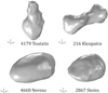 |
Fig. 10 Shapes of four asteroids. The spin axis goes through the barycentre (geometric centre) and is in the direction of the Z-axis. |
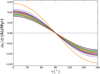 |
Fig. 11 Rate of semimajor axis drift da/dt versus the obliquity of the spin axis γ. Solid curves represent simulated results for 34 asteroids of 10 m radius with real shapes while the dashed curve represents the analytical result from the linear model for a 10 m-radius sphere. |
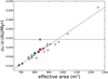 |
Fig. 12 Semimajor axis drift rate versus effective area (see text). The red solid triangle stands for the numerical results of a spherical asteroid and the red star is from the linear model for the same asteroid. The solid line is the least squares fit of the results for 34 shapes. |
4 Conclusions
In the past three decades, observations have shown the importance of the Yarkovsky effect on the motions of small celestial bodies. The recoil force of thermal irradiation may modify the rotation and orbit of asteroids, and semimajor axis drift is the most prominent long-term effect.
The linear model proposed by Vokrouhlický (1998a,b) has been widely adopted and has successfully produced good estimations for Yarkovsky effects on asteroid populations. In the linear model, the temperature variation on the asteroid surface (∆T) is assumed to be so small that  can be approximated by
  , and asteroids are assumed to be spherical or almost spherical. However, these two conditions could deviate in reality. In this paper, using multiphysics software COMSOL, we numerically calculate the diurnal Yarkovsky effect in three dimensions and make comparisons with the results derived from the linear model.
In the calculations, we find that the radiation flux from the Sun only introduces temperature fluctuation in a thin layer under the surface of the asteroid. Depending on the thermal conductivity, the thickness of this thermally affected-layer, beneath which the temperature is constant, is about ten times the penetration depth. Therefore, the numerical calculation of surface temperature that determines the Yarkovsky effect can be performed in this subsurface layer, that is, the asteroid can be regarded as the combination of a thermally affected shell and an isothermal core.
After obtaining the temperature distribution numerically, we calculate the Yarkovsky force or the semimajor axis drift rate. Comparisons with results derived from the linear model show that the linear model for spherical bodies works very well, with the relative errors being within 10% in most cases. However, the linear model could moderately deviate from the real situation when the asteroid is a poor conductor of heat (low conductivity) or is very close to the Sun.
The thermal inertia Γ indicates the capacity to store energy and to delay the transmission of heat in the material. We find that Γ dictates the strength of the diurnal Yarkovsky effect for large bodies. However, when the asteroid is so small – or equivalently the thermal conductivity is so large – that its size is comparable to the penetration depth, the Yarkovsky effect is not decided by Γ alone. Another thermal parameter Θ, which specifies the body’s ability to retain temperature changes over a rotation period, may control the delay angle between the subsolar point and the hottest spot on the surface, and thus determines the ratio between radial and transverse components of the Yarkovsky force.
Compared to a sphere, a prolate biaxial ellipsoid produces a stronger diurnal effect, while an oblate ellipsoid has a weaker effect. The results derived from the linear model for biaxial ellipsoids are overall consistent with numerical simulations. However, a systematic overestimation of the transverse Yarkovsky force can be found in the linear model, and the deviation is greater for oblate ellipsoids.
For triaxial ellipsoids, we find the diurnal Yarkovsky effect to be a periodic effect, for which no theoretical solution is now available. Within one rotation period, the transverse Yarkovsky force could change direction, from positive to negative and vice versa. Our numerical results show that a triaxial ellipsoid always receives a stronger average diurnal Yarkovsky effect than that acting on the biaxial ellipsoid with the same volume and flattening parameter e1. When a linear model is used to calculate the effect, the deviation from numerical results may reach 40%, depending on the flattening parameters.
Apart from these fictitious regular shapes, we also considered 34 real shapes, many of which are extremely irregular. Our calculations show that the semimajor axis drift rates tend to be overestimated by 16% on average and up to 35% if the linear model for spheres is applied. We introduce the ‘effective area’ to quantify the relative diurnal Yarkovsky effect on irregularly shaped asteroids, and we find a perfect linear relationship between the semimajor axis drift rate and the effective area. For an asteroid of any shape, by comparing its effective area with that of a standard model (e.g. a spherical asteroid), the Yarkovsky effect can be obtained directly without calculating the temperature distribution on the surface assuming the same thermal parameters. Combined with our analysis of the deviation of the linear model for the Yarkovsky effect, the effective area provides an efficient approach to accurately calculate the Yarkovsky effect for asteroids of irregular shapes analytically.
The effective area defined here reflects only the geometrical property of the surface, and the shadowing effect has been neglected; we also assume that the heat transfer is localised. These assumptions are reasonable for the majority of real asteroids, given that the penetration depth is much smaller than the radius. However, the effective area for asteroids of extremely irregular shape and/or showing complicated rotation needs to be improved. Similarly, an ‘effective torque’ can also be defined to estimate the YORP effect, which will be discussed in a separate paper.
Acknowledgements
We thank the anonymous referee for the valuable comments. This work has been supported by the National Key R&D Program of China (2019YFA0706601) and National Natural Science Foundation of China (NSFC, Grants No.11933001 & No.11473016). We also acknowledge the science research grants from the China Manned Space Project with No.CMS-CSST-2021-B08. J.Y.L.’s contribution to this work is not supported by any funds. The temperature distribution on the asteroid’s surface is computed using COMSOL software.
References
- Afonso, G. B., Gomes, R. S., & Florczak, M. A. 1995, Planet. Space Sci., 43, 787 [NASA ADS] [CrossRef] [Google Scholar]
- Basart, J., Goetzke, E., Setzer, C., & Wie, B. 2012, in AIAA/AAS Astrodynamics Specialist Conference, 5058 [Google Scholar]
- Beekman, G. 2005, J. British Astron. Assoc., 115, 207 [NASA ADS] [Google Scholar]
- Beekman, G. 2006, J. History Astron., 37, 71 [NASA ADS] [CrossRef] [Google Scholar]
- Bottke, W. F., Vokrouhlický, D., Brož, M., Nesvorný, D., & Morbidelli, A. 2001, Science, 294, 1693 [NASA ADS] [CrossRef] [Google Scholar]
- Capek, D., & Vokrouhlický, D. 2005, IAU Colloq., 197, 171 [Google Scholar]
- Chesley, S. R., Ostro, S. J., Vokrouhlický, D., et al. 2003, Science, 302, 1739 [NASA ADS] [CrossRef] [Google Scholar]
- Delbo, M., Mueller, M., Emery, J. P., Rozitis, B., & Capria, M. T. 2015, Asteroids IV, Asteroid Thermophysical Modeling (Tucson: University of Arizona Press), 107 [Google Scholar]
- Farinella, P., & Vokrouhlický, D. 1999, Science, 283, 1507 [CrossRef] [Google Scholar]
- Farinella, P., Vokrouhlický, D., & Hartmann, W. K. 1998, Icarus, 132, 378 [NASA ADS] [CrossRef] [Google Scholar]
- Ferrari, S. 2007, in 2nd PALENC Conference and 28th AIVC Conference on Building Low Energy Cooling and Advance Ventilation Technologies in the 21st Century, Greece, 346–351 [Google Scholar]
- Groath, D. J., Basart, J. P., & Wie, B. 2014, in AIAA/AAS Astrodynamics Specialist Conference, 4145 [Google Scholar]
- Hyland, D. C., Altwaijry, H. A., Ge, S., et al. 2010, Cosmic Res., 48, 430 [NASA ADS] [CrossRef] [Google Scholar]
- Nesvorný, D., & Bottke, W. F. 2004, Icarus, 170, 324 [Google Scholar]
- Öpik, E. J. 1951, Proc. R. Irish Acad. Sect. A, 54, 165 [Google Scholar]
- Palluconi, F. D., & Kieffer, H. H. 1981, Icarus, 45, 415 [NASA ADS] [CrossRef] [Google Scholar]
- Peterson, C. 1976, Icarus, 29, 91 [NASA ADS] [CrossRef] [Google Scholar]
- Radzievskii, V. V. 1952, AZh, 29, 162 [NASA ADS] [Google Scholar]
- Rozitis, B., & Green, S. F. 2011, MNRAS, 415, 2042 [NASA ADS] [CrossRef] [Google Scholar]
- Rubincam, D. P. 1987, J. Geophys. Res., 92, 1287 [NASA ADS] [CrossRef] [Google Scholar]
- Scholl, H., Marzari, F., & Tricarico, P. 2005a, Icarus, 175, 397 [NASA ADS] [CrossRef] [Google Scholar]
- Scholl, H., Marzari, F., & Tricarico, P. 2005b, AJ, 130, 2912 [NASA ADS] [CrossRef] [Google Scholar]
- Sekiya, M., Shimoda, A. A., & Wakita, S. 2012, Planet. Space Sci., 60, 304 [NASA ADS] [CrossRef] [Google Scholar]
- Spencer, J. R., Lebofsky, L. A., & Sykes, M. V. 1989, Icarus, 78, 337 [Google Scholar]
- Spitale, J. N. 2002, Science, 296, 77 [NASA ADS] [CrossRef] [Google Scholar]
- Spitale, J. N., & Greenberg, R. 2001, Icarus, 149, 222 [NASA ADS] [CrossRef] [Google Scholar]
- Spitale, J. N., & Greenberg, R. 2002, Icarus, 156, 211 [NASA ADS] [CrossRef] [Google Scholar]
- Spoto, F., Milani, A., & Kneževic, Z. 2015, Icarus, 257, 275 [NASA ADS] [CrossRef] [Google Scholar]
- Tsiganis, K., Varvoglis, H., & Morbidelli, A. 2003, Icarus, 166, 131 [NASA ADS] [CrossRef] [Google Scholar]
- Vokrouhlický, D. 1998a, A&A, 335, 1093 [Google Scholar]
- Vokrouhlický, D. 1998b, A&A, 338, 353 [NASA ADS] [Google Scholar]
- Vokrouhlický, D. 1999, A&A, 344, 362 [NASA ADS] [Google Scholar]
- Vokrouhlický, D., & Farinella, P. 1998, AJ, 116, 2032 [CrossRef] [Google Scholar]
- Wang, J., Bras, R. L., Sivandran, G., & Knox, R. G. 2010, Geophys. Res. Lett., 37, L05404 [NASA ADS] [Google Scholar]
- Wesselink, A. J. 1948, Bull. Astron. Inst. Netherlands, 10, 351 [Google Scholar]
- Xu, Y.-B., Zhou, L.-Y., & Ip, W.-H. 2020a, A&A, 637, A19 [NASA ADS] [CrossRef] [EDP Sciences] [Google Scholar]
- Xu, Y.-B., Zhou, L.-Y., Lhotka, C., & Ip, W.-H. 2020b, MNRAS, 493, 1447 [CrossRef] [Google Scholar]
- Xu, Y.-B., Zhou, L., Lhotka, C., Zhou, L.-Y., & Ip, W.-H. 2022, A&A, submitted [arXiv:2206.06114] [Google Scholar]
- Zhao, Y., Ji, J., Huang, J., et al. 2015, MNRAS, 450, 3620 [CrossRef] [Google Scholar]
- Zhou, L., Xu, Y.-B., Zhou, L.-Y., Dvorak, R., & Li, J. 2019, A&A, 622, A97 [NASA ADS] [CrossRef] [EDP Sciences] [Google Scholar]
COMSOL Multiphysics® v. 5.6. www.comsol.com. COMSOL AB, Stockholm, Sweden.
All Figures
|
Fig. 1 Temperature along a certain radius on the equatorial plane at four different times. The depth is measured downwards from the surface. |
| In the text | |
|
Fig. 2 Influence of adopted shell thickness on the simulated results. Upper panel: temperature distribution along the equator for two values of shell thickness. Lower panel: dependence of the simulated transverse Yarkovsky force on the adopted shell thickness. |
| In the text | |
|
Fig. 3 Comparisons of the Yarkovsky forces derived from the linear model (theoretical) and numerical simulations for varying density ρ. Upper panel: forces (blue for radial and red for transverse components) versus ρ. Solid curves refer to simulated results while dashed curves are for the linear model. Lower panel: fractional differences between the results from two methods. Blue and red curves are for the radial and transverse components, while grey and light-grey areas indicate the difference of less than 5 and 10%, respectively. |
| In the text | |
|
Fig. 4 Same as Fig. 3 but for varying thermal conductivity K. In the upper panel, the vertical orange dotted line refers to the location of Θ = 1 while the vertical grey dashed line indicates where the penetration depth is equal to the radius of the asteroid. |
| In the text | |
|
Fig. 5 Transverse Yarkovsky force of asteroids with given Γ but different sets of ρ, C, and K (see text). The dotted line refers to R/ls = 1. |
| In the text | |
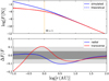 |
Fig. 6 Same as Fig. 4 but for varying heliocentric distance r. |
| In the text | |
|
Fig. 7 Yarkovsky forces acting on biaxial ellipsoids and the difference between the linear model and numerical simulations. Upper panel: ratio of the forces acting on ellipsoids F1 to those on the sphere F0 versus oblateness e1. Lower panel: relative differences between the forces derived from the linear model and numerical simulations. Blue and red mark the radial and transverse components, respectively. |
| In the text | |
|
Fig. 8 Evolutions of the radial force (blue) and transverse force (red) acting on a triaxial ellipsoid in one rotation period. The flattening parameters e1 = 0.3 and e2 = 3. |
| In the text | |
|
Fig. 9 Ratio of the forces acting on triaxial ellipsoids F2 to those on biaxial ellipsoids of the same volume F1 versus the flattening parameters e1 and e2. Blue and red are for radial and transverse forces, while solid circles, triangles, and squares refer to e1 = 0.3, 1, and 3, respectively. |
| In the text | |
|
Fig. 10 Shapes of four asteroids. The spin axis goes through the barycentre (geometric centre) and is in the direction of the Z-axis. |
| In the text | |
|
Fig. 11 Rate of semimajor axis drift da/dt versus the obliquity of the spin axis γ. Solid curves represent simulated results for 34 asteroids of 10 m radius with real shapes while the dashed curve represents the analytical result from the linear model for a 10 m-radius sphere. |
| In the text | |
|
Fig. 12 Semimajor axis drift rate versus effective area (see text). The red solid triangle stands for the numerical results of a spherical asteroid and the red star is from the linear model for the same asteroid. The solid line is the least squares fit of the results for 34 shapes. |
| In the text | |
Current usage metrics show cumulative count of Article Views (full-text article views including HTML views, PDF and ePub downloads, according to the available data) and Abstracts Views on Vision4Press platform.
Data correspond to usage on the plateform after 2015. The current usage metrics is available 48-96 hours after online publication and is updated daily on week days.
Initial download of the metrics may take a while.