| Issue |
A&A
Volume 690, October 2024
|
|
|---|---|---|
| Article Number | A33 | |
| Number of page(s) | 15 | |
| Section | Interstellar and circumstellar matter | |
| DOI | https://doi.org/10.1051/0004-6361/202345986 | |
| Published online | 26 September 2024 | |
ALMA-IMF
XV. Core mass function in the high-mass star formation regime
1
Univ. Grenoble Alpes, CNRS, IPAG,
38000
Grenoble,
France
2
DAS, Universidad de Chile,
1515 camino el observatorio, Las Condes,
Santiago,
Chile
3
National Astronomical Observatory of Japan, National Institutes of Natural Sciences,
2-21-1 Osawa, Mitaka,
Tokyo
181-8588,
Japan
4
Department of Astronomical Science, SOKENDAI (The Graduate University for Advanced Studies),
2-21-1 Osawa, Mitaka,
Tokyo
181-8588,
Japan
5
Departamento de Astronomía, Universidad de Concepción,
Casilla 160-C,
Concepción,
Chile
6
Franco-Chilean Laboratory for Astronomy, IRL 3386, CNRS and Universidad de Chile,
Santiago,
Chile
7
Université Paris-Saclay, Université Paris Cité, CEA, CNRS, AIM,
91191
Gif-sur-Yvette,
France
8
Instituto de Radioastronomía y Astrofísica, Universidad Nacional Autónoma de México,
Morelia,
Michoacán
58089,
Mexico
9
Laboratoire d’astrophysique de Bordeaux, Univ. Bordeaux, CNRS,
B18N, allée Geoffroy Saint-Hilaire,
33615
Pessac,
France
10
Department of Astronomy, University of Florida,
PO Box 112055,
Florida,
USA
11
Herzberg Astronomy and Astrophysics Research Centre, National Research Council of Canada,
5071 West Saanich Road,
Victoria,
BC V9E 2E7,
Canada
12
Laboratoire de Physique de l’École Normale Supérieure, ENS, Université PSL, CNRS, Sorbonne Université, Université de Paris,
Paris,
France
13
SKA Observatory, Jodrell Bank, Lower Withington,
Macclesfield
SK11 9FT,
UK
14
Departments of Astronomy and Chemistry, University of Virginia,
Charlottesville,
VA
22904,
USA
15
Observatoire de Paris, PSL University, Sorbonne Université, LERMA,
75014,
Paris,
France
16
INAF – Osservatorio Astrofisico di Arcetri,
Largo E. Fermi 5,
50125
Firenze,
Italy
17
Departament de Física Quàntica i Astrofísica (FQA), Universitat de Barcelona (UB),
c. Martí i Franquès, 1,
08028
Barcelona,
Spain
18
Institut de Ciències del Cosmos (ICCUB), Universitat de Barcelona (UB),
c. Martí i Franquès, 1,
08028
Barcelona,
Spain
19
Institut d’Estudis Espacials de Catalunya (IEEC),
08340,
Barcelona,
Catalonia,
Spain
20
Institute of Astronomy, National Tsing Hua University,
Hsinchu
30013,
Taiwan
21
Instituto Argentino de Radioastronomía (CCT-La Plata, CONICET; CICPBA),
C.C. No. 5, 1894, Villa Elisa,
Buenos Aires,
Argentina
22
Department of Astronomy, Yunnan University,
Kunming
650091,
PR China
23
Shanghai Astronomical Observatory, Chinese Academy of Sciences,
80 Nandan Road,
Shanghai
200030,
PR China
24
Steward Observatory, University of Arizona,
933 North Cherry Avenue,
Tucson,
AZ
85721,
USA
25
S. N. Bose National Centre for Basic Sciences,
Block JD, Sector III, Salt Lake,
Kolkata
700106,
India
26
ESO Headquarters,
Karl-Schwarzchild-Str 2,
85748
Garching,
Germany
27
Institut de Radioastronomie Millimétrique (IRAM),
300 rue de la Piscine,
38406
Saint-Martin-D’Hères,
France
28
National Radio Astronomy Observatory,
PO Box O,
Socorro,
NM
87801,
USA
Received:
24
January
2023
Accepted:
24
July
2024
Abstract
The stellar initial mass function (IMF) is critical to our understanding of star formation and the effects of young stars on their environment. On large scales, it enables us to use tracers such as UV or Hα emission to estimate the star formation rate of a system and interpret unresolved star clusters across the Universe. So far, there is little firm evidence of large-scale variations of the IMF, which is thus generally considered “universal”. Stars form from cores, and it is now possible to estimate core masses and compare the core mass function (CMF) with the IMF, which it presumably produces. The goal of the ALMA-IMF large programme is to measure the core mass function at high linear resolution (2700 au) in 15 typical Milky Way protoclusters spanning a mass range of 2.5 × 10³ to 32.7 × 10³ M⊙. In this work, we used two different core extraction algorithms to extract ≈680 gravitationally bound cores from these 15 protoclusters. We adopted a per core temperature using the temperature estimate from the point-process mapping Bayesian method (PPMAP). A power-law fit to the CMF of the sub-sample of cores above the 1.64 M⊙ completeness limit (330 cores) through the maximum likelihood estimate technique yields a slope of 1.97 ± 0.06, which is significantly flatter than the 2.35 Salpeter slope. Assuming a self-similar mapping between the CMF and the IMF, this result implies that these 15 high-mass protoclusters will generate atypical IMFs. This sample currently is the largest sample that was produced and analysed self-consistently, derived at matched physical resolution, with per core temperature estimates, and cores as massive as 150 M⊙. We provide both the raw source extraction catalogues and the catalogues listing the source size, temperature, mass, spectral indices, and so on in the 15 protoclusters.
Key words: methods: observational / techniques: interferometric / stars: formation / ISM: clouds / ISM: structure / submillimeter: ISM
Corresponding author; This email address is being protected from spambots. You need JavaScript enabled to view it.
© The Authors 2024
 Open Access article, published by EDP Sciences, under the terms of the Creative Commons Attribution License (https://creativecommons.org/licenses/by/4.0), which permits unrestricted use, distribution, and reproduction in any medium, provided the original work is properly cited.
This article is published in open access under the Subscribe to Open model. This email address is being protected from spambots. You need JavaScript enabled to view it. to support open access publication.
1 Introduction
In 1955, Edwin Salpeter reported that the high-mass tail of the initial mass function of stars, the IMF, could be represented by a power law of the form  with α = 2.35. Since then, numerous studies reported its universality (see the review by Bastian et al. 2010) and studied its origin (e.g. Hennebelle & Chabrier 2008). To investigate the origin of the IMF, astronomers studied the fragmentation of molecular clouds in the form of small substructures (≲0.03 pc; the cores) and the link between the core mass function (CMF) and the IMF (e.g. Motte et al. 1998; Fiorellino et al. 2021). Because of observational limitations, these studies focused mostly on nearby clouds (≈140–400 pc) until 2018. These clouds mainly form low- and intermediate-mass stars. All studies reported CMF slopes at the high-mass end that were compatible with the slope of the IMF, suggesting that the IMF directly inherits its shape from the CMF (e.g. Alves et al. 2007; Könyves et al. 2010).
In 2018, taking advantage of the angular resolution and sensitivity of the Atacama Large Millimetre/submillimetre Array (ALMA), Motte et al. (2018) studied the high-mass protocluster W43-MM1 at a distance of ≃5.5 kpc. They reported a CMF with a high-mass tail that was flatter than the canonical IMF, with α=1.96±0.13. Since then, other teams have reported similar results in other high-mass protoclusters, but often used singlepointing observations, thus narrow fields that do not image parsec-scale clouds (e.g. Liu et al. 2018; Cheng et al. 2018; Kong 2019; O’Neill et al. 2021). These results cast doubt on the universality of the IMF, on a direct link between the CMF and the IMF, or on both. However, the comparison of core samples between these studies, which are captured at different evolutionary stages, becomes complex or impossible when the observations are carried out at disparate physical resolutions and/or sensitivities. Thus, it became imperative to obtain a sample of high-mass protoclusters that are representative of the Milky Way and were observed homogeneously.
To directly address this, we present in this article the results of the ALMA-IMF Large Program (PIs: F. Motte, A. Ginsburg, F. Louvet, P. Sanhueza). ALMA-IMF observed 15 high-mass protoclusters at comparable sensitivity and physical resolution. The main driver of the protocluster selection is a mass criterion that first chose protoclusters with inner parts of at least 500 M⊙, as described in detail in Sect. 2.1 of Motte et al. (2022).
A second criterion was the distance of the protoclusters. Not too close by (>2 kpc) to permit imaging a large area with mosaic observations, and not too far (<6 kpc) to prevent excessive integration time. Our final sample consists of 15 protoclusters that were observed with a continuum sensitivity below 60 mK at 1.3 mm, and at similar physical resolution (≈2 kau).
In this article, we determine and analyse the combined CMF of all 15 protoclusters from ALMA-IMF. We show the 1.3 and 3 mm continuum images in Sect. 2; they were first presented in Ginsburg et al. (2022). We describe the source extraction in Sect. 3. We describe the source selection and core mass derivation in Sect. 4, paying special attention to free-free emission and to the core temperatures. We present the global CMF for all 15 fields. We discuss our results regarding the current knowledge about the CMF in Sect. 6, and we summarise our conclusions in Sect. 7.
General properties of the ALMA-IMF fields.
2 Observations
The data were taken from the ALMA-IMF large programme (Project ID: 2017.1.01355.L), entitled ALMA transforms our view of the origin of stellar masses. Motte et al. (2022), hereafter referred to as Paper I, described the project, its choice of targets, datasets, objectives, and first results. Ginsburg et al. (2022), hereafter referred to as Paper II, described the reduction pipeline for the continuum emission maps at 1.3 mm and 3 mm in the ALMA-IMF sample. Paper II presented two versions of the continuum maps: the BSENS and the CLEANEST. The BSENS maps were constructed using the full range of the continuum spectral windows, which may include significant molecular emission, especially toward hot cores. The CLEANEST maps were constructed by flagging all channels contaminated by molecular emission (see Fig. 3 in Paper II). Because we wish to assemble the most reliable sample of cores, we used the CLEANEST continuum maps, which are publicly available on the ALMA-IMF website1. Table 1 lists the 15 regions investigated by ALMA-IMF together with the observational characteristics taken from Papers I and II that are relevant to the present paper. We refer to Paper I for an in-depth description of the 15 regions.
3 Source extraction
3.1 Extraction tools
To extract sources in the continuum emission maps, we used two extraction tools: getsf (v210414, Men’shchikov 2021b) and GExt2D (v210603, Bontemps et al., in prep.). This approach permitted us to assess the biases inherent to our source extraction algorithms.
The multi-scale multi-wavelength source and filament extraction method getsf supersedes the previous algorithms getsources, getfilaments, and getimages (Men’shchikov et al. 2012; Men’shchikov 2013, 2017, respectively). The getsf method separates the structural components of sources, filaments, and background in the observations into independent images of the different components. Source and filament extraction are performed with their respective images, where the contributions of the other components are largely removed. For more details on getsf, illustrations of its applications, quantitative extraction performance, and comparisons with getsources, we refer to Men’shchikov (2021a,b).
GExt2D is based on the same idea as the cutex tool (Molinari et al. 2011). As a first step, it uses the second derivative of the maps to identify the locations of maximum curvature as indicative of compact sources. It starts from the strongest curvatures down to fainter and shallower fluctuations close to those expected from measured local noise. The second step involves source boundary identification and removal of background emission as the interpolated values in the map inside the boundaries. The third step corresponds to an automated Gaussian fitting at each location of compact sources after subtracting the derived background.
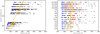 |
Fig. 1 Scatter plots of the source size (black dots) extracted with getsf before (left) and after (right) the maps were smoothed to a homogeneous spatial resolution of 2700 au. The blue triangles display the beam sizes. The orange diamonds display the mean sizes of sources. In the left panel, the y-axis is the linear scale (beam × distance) of the maps in Band 6, and the orange line shows the fit to the mean source size distribution for each field. In the right panel, the orange line shows the mean core size of all 15 protoclusters, and the red crosses illustrate the cores exceeding 25 M⊙. |
3.2 Source extraction at native angular resolutions
With both getsf and GExt2D, the source extraction strategy has the same two steps. Firstly, we detected source candidates in the continuum images at 1.3 mm (Band 6) without primary-beam correction. These images have a homogeneous noise level in the entire field. This choice permits the detection of sources with a constant signal-to-noise ratio threshold. Secondly, we measured the source fluxes and sizes in the continuum maps at 1.3 mm and 3 mm (Band 3) after primary-beam correction. In this way, the fluxes we obtained account for any attenuation resulting from being farther from the phase centre of the fields. This strategy replicates that applied in Pouteau et al. (2022), hereafter referred to as Paper III, dedicated to the W43-MM2 and W43-MM3 protoclusters. Considering all 15 protoclusters together, we extracted 820 sources with getsf, and 930 with GExt2D. GExt2D detects the sources in the observed image, while getsf decomposes the image first and requires detecting a source in successive scales to validate its detection. Hence, getsf is more conservative and extracts fewer sources than GExt2D.
The distances of the protoclusters range from 2.5 to 5.5 kpc (see Table 1 in Paper I). The ALMA-IMF large programme aimed to image the 15 protoclusters with the same spatial resolution of 2100 au, requesting the corresponding angular resolution for each field. Despite this effort, the available antenna configurations at the observatory led to variations in the spacial resolutions by up to a factor of two (see Table 1 and Paper I). These variations in physical scale impact the size and mass of the sources that can be extracted. Louvet et al. (2021) performed convolution tests on projected density cubes obtained from hydro-dynamical simulations and on column density maps created from Herschel observations and showed that the sizes and integrated fluxes of the extracted sources closely follow the size of the linear scale. The left panel of Fig. 1 shows a linear dependence between the mean source size and the linear resolution. To obtain a homogeneous sample of sources, the data must be smoothed to a matched spatial resolution.
3.3 Source extraction at matched physical resolution
To extract a spatially homogeneous core sample, we smoothed the 1.3 and 3 mm maps to the lowest native resolution of ≃2700 au. We convolved each map with a Gaussian kernel whose width, θconv, was calculated as
 (1)
(1)
where D is the distance to the target expressed in parsecs, and θnative is the native angular resolution of the map. Table 2 lists the angular resolution of each field after smoothing. We present the smoothed continuum emission maps at 1.3 mm in Fig. 2.
We adopted the same strategy as explained in Sect. 3.2 to extract sources in the smoothed maps. In total, we retrieved about 680 sources with getsf and 1020 with GExt2D 2. Table 2 lists the number of sources extracted per field with both algorithms, and Fig. 2 shows the sources extracted with getsf3. The right panel of Fig. 1 shows the sizes of the sources we extracted with getsf for each field. The mean size is similar for each field with L = 3 840 ± 270 au4.
4 Results
4.1 Getsf versus GExt2D extraction methods
In total, we retrieved 677 sources with getsf, and 1020 with GExt2D. The agreement between these extractions is good because ≈80% of the sources found by getsf are also found by GExt2D (Table 2). To compare the source flux measurements, we constructed the source flux functions (SFFs) and complementary cumulative SFFs for both algorithms (Fig. 3). The first function shows that the source fluxes range between 10 mJy and 10Jy for both algorithms, with a similar median value at ≃12mJy. It also shows that the additional sources found by GExt2D are low- and intermediate-flux sources from ≈30mJy to 200 mJy. The complementary SFF permitted us to estimate the slope of the high-flux end of the SFF. We fitted the cumulative SFF with a power law from the median value of the samples, that is, 12 mJy, up to the flux at which the number of cores is below ten5. The fitted high-flux slopes are similar for both catalogues, with ζ′ ≃ 0.85. These exponents, adjusted onto the complementary cumulative SFFs, correspond to power laws with exponents ζ = ζ′ + 1 ≃ 1.85. This analysis proves that the overall statistics of the source flux are independent of the two extraction algorithms we employed. In the following, we choose to focus on the extractions performed by getsf since it is more conservative than GExt2D, which is confirmed by the large fraction of getsf sources confirmed with GExt2D. When we compare the sources extracted at the native angular resolutions (see Sect. 3.2) to the sources extracted in the smoothed maps (see Sect. 3.3), the agreement between the getsf catalogues is better than that between GExt2D catalogues. About 95% of the sources extracted in the smoothed maps were also extracted at the native angular resolutions with the getsf algorithm. This fraction drops to ≃75% in the case of the GExt2D extractions.
Resolutions, noise levels, and sources extracted after smoothing to a linear scale of 2700 au.
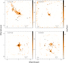 |
Fig. 2 Fifteen ALMA-IMF protoclusters as traced by their continuum emission at 1.3 mm at a matched spatial resolution of 2700 au. The ellipses locate all the cores found by getsf. The name of the field is indicated in the top left corner of each panel, and the beam size is shown in the bottom left corner. For each protocluster, the centre coordinates are those specified in Table 1. We show the remaining fields in Fig. A.1. |
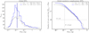 |
Fig. 3 Source flux distributions for the getsf and GExt2D source extractions. The left panel displays the SFFs of the sources extracted by getsf in grey and by GExt2D in blue. The vertical blue and grey lines indicate the median values for each source catalogues, which differ by ≃5%. The right panel displays the complementary cumulative SFFs from the getsf source extraction (in grey) and from the GExt2D source extraction (in blue). The grey and blue lines display the best fits from linear regressions on the complementary cumulative SFFs from the median value at 12 mJy up to the flux at which the number of cores is smaller than 10. The corresponding ζ power-law indexes are indicated in the top right corner. |
4.2 From source flux to core mass
4.2.1 Removing contaminated sources
The integrated fluxes comprise thermal dust emission and potentially free-free emission for the more evolved sources. In the following, we filter the sources that are arguably contaminated by free-free emission. To do this, we used the integrated flux measurements at 1.3 and 3 mm, when available, to compute their spectral index. To correct for the source size differences between 1.3 and 3 mm extractions, we linearly adjusted the integrated fluxes at 3mm:  , where ΘA and ΘB are the major and minor axes of the sources at 1.3 or 3 mm, respectively. This operation corrected the 3 mm fluxes by 17% on average. This flux rescaling replicates the method we used in Paper III. This rescaling works for an optically thick emission, and an optically thin emission for an isothermal protostellar envelope with a density profile ρ(r) ∝ r−2, where r is the radius of the envelope. We then computed the spectral index as
 (2)
(2)
where v1.3mm and v3mm are the central frequencies of the ALMA Band 6 and Band 3, respectively (see Table 1). We removed 68 sources with γ < 2, which are presumably contaminated by free-free emission. These sources are represented by the pink ellipses in Fig. 4.
To investigate the ≃500 sources that lack measurements at 3 mm, we built the spectral index map for each field using Eq. (2) on a pixel-by-pixel basis by replacing  with the pixel intensities. We point out that the angular resolutions and pixel sizes of the images at 1.3 mm equal that of the images at 3 mm. We show the spectral index maps in Fig. 4. The red areas (γ > 2) represent pixels with thermal dust emission, those in green (0 < γ < 2) pixels contaminated by free-free emission, and those in blue (γ < 0) pixels dominated by free-free emission. We manually selected all the sources lying over free-free emission areas (γ < 2; see yellow ellipses in Fig. 4). For the sources that are undetected at 3 mm, we estimated their flux,
  , using the integrated flux in the aperture corresponding to the footprint of the source detected at 1.3 mm. We emphasise that although getsf did not detect these 1.3 mm sources as compact sources at 3 mm, they do have a background emission above 3σ at 3 mm by definition of the spectral index maps. We used this upper limit to compute an upper limit on their spectral index as
 (3)
(3)
and we rejected the 16 sources with a spectral index below one, those for which free-free emissions could substantially contribute to the emission.
This filtering rejected 84 of the 677 sources extracted by getsf. The degree of rejection depended on the evolutionary stages of the regions: ≃0.5% in the young regions, ≃10% in the intermediate regions, and ≃25% in the evolved regions. Table 3 lists the number of sources that were rejected when these two levels of filtering were applied for each field.
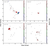 |
Fig. 4 Maps of the spectral index in the 15 ALMA-IMF fields. We chose the colours such that red traces dust thermal emission, blue traces free-free emission, and green likely traces a mixture of dust and free-free emissions. The maps display the spectral index value only where the 3 mm intensity exceeds 3 σ. The black ellipses display the sources extracted by getsf. We show the remaining fields in Fig. B.1. |
4.2.2 Core temperatures
Following the pilot study by Motte et al. (2018), we used the Bayesian procedure PPMAP (Marsh et al. 2015; Dell’Ova et al. 2024) to build the temperature maps of the ALMA-IMF protoclusters. The procedure uses several continuum emission maps to compute a cube of column densities as a function of dust temperature. Along with the ALMA data in Band 6 decontaminated from free-free emission (Galván-Madrid et al. 2024), our PPMAP execution takes the following maps as input:
SOFIA/HAWC+ data at 214 µm with an angular resolution of 19.0″ (only for G012.80, G351.77, W51-E, and W51-IRS2, Vaillancourt 2016; Pillai & Simplifi Team 2023).
Herschel/PACS and Herschel/SPIRE data at 70, 160, 250, 350, and 500 µm with angular resolutions of 5.6, 10.7, 17.6, 23.9, and 35.2″, respectively (Molinari et al. 2010; Motte et al. 2010).
APEX/SABOCA data at 350 µm with an angular resolution of 7.8″ (Lin et al. 2019).
APEX/LABOCA data at 870 µm with an angular resolution of 19.2″ (Schuller et al. 2009).
We refer to Dell’Ova et al. (2024) for an in-depth description of the method. Finally, we obtained a unique temperature for each core at an angular resolution of 2.5″. The derived temperatures vary from 19.4 to 62.8 K (see tables published on CDS). The error associated with the PPMAP derivation is ≈5 K; to account for potential systematic contributions, we adopted a 25% error on the PPMAP temperature estimates6.
We adopted the PPMAP temperatures for all cores except for the hot-core candidates, for which we adopted the method proposed in Bonfand et al. (2024): We cross-correlated the position of continuum sources (see Sect. 3.3) with methyl formate (CH3 OCHO) emission maps that were observed by ALMA-IMF. Methyl formate forms at the surface of dust grains in lukewarm (30–40 K) regions and is then released in the gas phase when the temperature reaches ≈100K (e.g. Garrod et al. 2009). Methyl formate can be used as a proxy to trace regions where heating is present and dust surface products have started to sublimate. Following the method discussed in Bonfand et al. (2024), we set 100±50 K to the 49 sources whose position corresponded to the peaks of extended methyl formate emission. These sources are classified as hot-core candidates.
Additionally, we set 300±100K to sources n°1, n°2, and n°1 in W51-IRS2, W51-E, and G327.29 respectively, following their detailed modelling by Ginsburg et al. (2017), Goddi et al. (2020), and the adopted temperature in Bonfand et al. (2024), respectively. These three sources are associated with strong and extended emission structures in the methyl formate emission maps7.
Evolution of the core sample through the selection process.
4.2.3 Core mass and boundedness
We converted the measured integrated flux at 1.3 mm,  , into a mass using the formula presented in Paper III, which includes a first-order correction for the optical thickness,
 (4)
(4)
where D is the distance to the target, K1.3mm = 0.1 (v/1000GHz)β cm2g−1 is the dust opacity per unit mass (dust + gas), with an opacity index β = 1.5 typical of cold and dense environments (Ossenkopf & Henning 1994), and B(T, v) is the Planck function computed at the representative frequency of the observations in Band 6 with the dust temperature T (see Table 1 for central frequencies and distances, and the tables published at the CDS for the source temperature).
Errors on the masses mostly arise from the uncertainties on the opacity index β and on the dust temperature, T. The masses would be a factor of two lower for β = 2 instead of β = 1.5. As for the temperature, a 25% difference leads to a mass shift by ≲40%.
To address the boundedness of cores, we computed the ratio MBE/Mcore, where Mcore is the core mass and MBE is the mass of the critical Bonnor-Ebert sphere (Bonnor 1956), whose size matches that of the core:  . Here, R is the equivalent core radius, estimated as
  8, where a and b are the major and minor axis of the source ellipse, respectively. Moreover, σth is the thermal broadening of lines, as
  , where γ = 1 is the adiabatic index (isothermal), kB is the Boltzmann constant, µ = 2.4 is the mean molecular weight per free particle, and mp is the mass of a proton. We considered the sources to be gravitationally bound when MBE/Msource < 2 (see e.g. Louvet et al. 2021). As listed in Table 3, this filter excludes no sources. We note that this is a first-order check of the boundedness of cores. A more accurate determination would require computing the equilibrium of each source taking into account its turbulence, external pressure, and magnetic field support in addition to the thermal support. Unfortunately, we lack all these pieces of information at the moment.
In Fig. 2, we show the thermal-dust cores for each field. The tables published at the CDS list all the sources detected by the getsf extraction algorithm in each field. The first group of sources in each table corresponds to thermal dust cores that are gravitationally bound, and the second group corresponds to sources whose fluxes are arguably contaminated by free-free emission. For each source, the last column indicates whether it was also detected by GExt2D, which is true for 80% of the extracted sources.
5 Core mass function
5.1 Completeness tests
In order to draw a coherent sample gathering cores from the 15 ALMA-IMF protoclusters, we need to ascertain that the core extractions are complete at the selected lower-mass limit. To do this, we performed completeness tests in each protocluster: We injected synthetic cores on top of their background emission (i.e. the emission subtracted from each source). The synthetic cores were injected in the form of 2D circular Gaussian with an FWHM corresponding to 3840 au, which is the mean core size (see Sect. 3.3). We injected these synthetic sources randomly provided the centres of the cores were separated by more than 2.5′′ . We forbid the injection of sources within 5′′ of the border of the maps, where the noise increases due to the primary-beam correction (see Fig. 2). The flux of the synthetic sources ranges from equivalent masses of 0.5 to 5 M⊙ in all fields for gas at 20 K, except in W51-E, where we adopted a mass range of 1 to 10 M⊙. The fluxes were equally split into ten flux bins. From these fluxes, we computed the mass of the synthetic cores when adopting the mean temperature of the cores extracted in the corresponding region. We then extracted the synthetic cores with the getsf method (see Sect. 3.1). To obtain good statistics in each mass bin, we repeated this procedure four times per field. Cumulating the four draws, we obtained ≃3800 cores in total in each field (or ≃380 per bin), and we probed ≃80% of the background area. We plot the percentage of synthetic cores we extracted as a function of their mass in the supplementary plots published on Zenodo. Following Paper III, we considered that the completeness limit was reached when 90% of the synthetic cores were extracted. The mass completeness varies from 0.80 to 1.64 M⊙ with a mean value of 1.34 M⊙ and a standard deviation of 0.2 M⊙. These numbers exclude W51-E, for which we find a completeness as high as 3.9 M⊙. We excluded W51-E from the analysis of the global CMF (see Sect. 6.1), and we restricted the core samples to cores exceeding 1.64 M⊙ to fit the high-mass tail of the CMF.
5.2 Fitting core mass functions
5.2.1 Method
The representation of a distribution in the form of histograms, as in Fig. 3, further fitted through linear regression, may give inaccurate results (Clauset et al. 2009). In addition, the representation in the form of a CMF in log-log scales prohibits us from estimating the fit uncertainty since the noise is not Gaussian. Moreover, the choice of the bin width induces a free parameter that thwarts any attempts to estimate the uncertainty. The representation in the form of a cumulative CMF, however, prevents us from estimating the uncertainty because the data are not independent. To circumvent these issues, we chose to fit the high-mass end of the CMF using maximum likelihood estimates (MLE). We followed the procedure presented by Clauset et al. (2009) and used its implementation in the Python package powerlaw presented by Alstott et al. (2014). When we assume that the CMF can be represented by a power law p(x) = Cx−α, where C is a constant, there must be some lower-mass value, xmin , from which the power-law fit is accurate and that prevents the divergence of p when x → 0. After normalisation (imposing that  ), this reads
 (5)
(5)
When xmin is known, the MLE gives an estimate of the exponent of the power law as
![Mathematical equation: $\alpha = 1 + n{\left[ {\mathop {\mathop \sum \nolimits^ }\limits_n^{i = 1} \ln {{{x_i}} \over {{x_{\min }}}}} \right]^{ - 1}},$](/articles/aa/full_html/2024/10/aa45986-23/aa45986-23-eq19.png) (6)
(6)
where xi is the mass of the core i (provided xi ≥ xmin), and the uncertainty on α reads
 (7)
(7)
where O is the mathematical notation for “not negligible in front of”.
The originality of the method by Clauset et al. (2009) is that it proposes a method for determining the best parameters xmin and α using the Kolmogorov-Smirnov (KS) distance. First, the method computes α for xmin taking successively each mass value of the core sample. Then it computes the maximal distance (the KS distance, KSD) between the observational CMF for all elements whose mass exceeds xmin and the synthetic CMF following a probability distribution function as defined by Eq. (5). The best value for the parameters xmin and α is the parameter that minimises the KSD. Figure 5 shows the evolution of α and KSD for all xmin values. In our case, we selected the highest value between the xmin that minimised the KSD and our completeness limit (see Sect. 5.1). The first minimum in the KSD was met for xmin =1.40 M⊙, below our completeness level at 1.64 M⊙. We therefore selected xmin = 1.64 M⊙, which corresponds to a core sample of 330 elements (excluding W51-E). From this subsample, we obtained a power-law index fit α = 2.11 ± 0.069. A sample of 330 cores above the completeness limit conveys a statistically conclusive sample. Clauset et al. (2009) reported stable index values when the sample exceeded ≈50 elements above the completeness limits. Consistently, Louvet et al. (2021) reported stable index values when the sample exceeded ≈40 elements above the completeness limits.
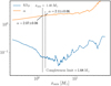 |
Fig. 5 Convergence towards the best fit of a power law through the MLE and KSD method for the global getsf bound core catalogue without the free-free sources. The left vertical dashed line highlights the first minimal KSD (in blue), occurring at xmin = 1.40 M⊙. The right vertical dashed line highlights the completeness limits at xmin = 1.64 M⊙. The orange curve shows the exponent of the power-law fit of the high-mass tail of the CMF as a function of xmin. |
5.2.2 Uncertainty of the fit
As pointed out in Sect. 4.2.3, errors in the mass estimates arise primarily from the uncertainties on the opacity index and core temperature. To study how these uncertainties affect the slope of the CMF, we performed a Monte Carlo simulation on our 330 cores by allowing their opacity index, their temperature, and their source flux to vary simultaneously. For the source flux, we used the Gaussian error associated with the flux measurement. Koen & Kondlo (2009) showed that including these errors on the fluxes flattens the distribution. However, since our relative uncertainty diminishes for brighter sources, we expect this effect to be marginal at the high-mass end of our CMF. In our Monte Carlo simulation, the opacity index β can take random normal values with a mean value of 1.5 (Ossenkopf & Henning 1994) and a standard deviation of 0.2 for each core. In parallel, we allowed the core temperature to take random normal values with the mean and standard deviation as described in Sect. 4.2.2. We show the resulting cumulative CMFs generated from 103 trials in Fig. 6. Each draw was fitted via MLE (see Sect. 5.2.1), fixing xmin to 1.64 M⊙. We obtain a mean exponent value for the slope of the CMF of 1.97±0.06, where the uncertainty is the quadratic sum of the statistical uncertainty from Eq. (7) (σ ≃ 0.06) and from the uncertainties on the temperature, opacity index, and flux measurement uncertainties (σ ≃ 0.02). We show in the supplementary plots published on Zenodo the results of the 103 trials for a power-law fit.
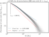 |
Fig. 6 The grey curves show the complementary cumulative CMFs of the 103 core samples obtained by including flux measurement uncertainties, varying core temperatures, and applying opacity index variations on a per-regions basis (see Sect. 5.2.2), overlaid with the average fit by a power law (in blue) and the best fit with a power-law index 2.35 (in red). |
5.2.3 Comparison with the Salpeter slope
The ALMA-IMF large programme aims to test whether the high-mass slope of the CMF differs from the high-mass slope of the canonical IMF (α = 2.35 when fitted by a power law; Salpeter 1955). To determine whether our sample of 330 cores (with M > xmin = 1.64 M⊙) permits such a claim, we selected 330 sources from a perfect mass distribution with an exponent of 2.35 and fitted the slope of its high-mass tail through the MLE. We repeated the operation 105 times. Figure 7 shows the probability of retrieving an exponent α when the parental distribution has a slope α = 2.35. With 330 cores, the probability of retrieving a slope compatible with ALMA-IMF, α = 1.97 ± 0.06, is lower than 1% (σ ≈ 2.4). Therefore, we report that the CMF in the protoclusters studied by ALMA-IMF is flatter than and cannot reasonably be reconciled with the Salpeter-IMF slope to a 2.4σ level10.
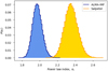 |
Fig. 7 Power-law exponents α retrieved when sorting 330 cores from a synthetic core sample whose CMF has a power-law exponent of 1.97 (in blue) and 2.35 (in orange). |
6 Discussion
6.1 Global top-heavy core mass function
In Sects. 5.2.1 and 5.2.2, we presented the best fit to the high-mass tail of the CMF by a power law. The best fit yields α = 1.97 ± 0.06. This result, based on 330 cores, confirms the many investigations conducted in recent years that reported top-heavy CMFs in high-mass protoclusters (e.g. Motte et al. 2018; Cheng et al. 2018; Sanhueza et al. 2019; Kong 2019; Moser et al. 2020). We show that this slope cannot be reconciled, at the 2.4σ level, with the canonical IMF slope (α = 2.35, see Sect. 5.2.3) even after the inclusion of all known uncertainties.
Observing top-heavy CMFs in high-mass protoclusters contrasts with nearby low-mass star-forming regions where a high-mass tail compatible with Salpeter is consistently found (see e.g. Table 6 of Fiorellino et al. 2021 for all CMF exponents from the Herschel Gould Belt Survey).
6.2 From the core mass function to the initial mass function
To link the CMF to the IMF, one must assume that cores constitute the mass reservoir for the accretion of protostars. One also assumes a fragmentation cascade and a mass transfer efficiency ϵ from the cores to the protostars. The common assumption for protostars is that one core will give birth to one star (and therefore assumes no sub-fragmentation) and that ϵ remains constant regardless of the core mass. If we adopt these assumptions, our massive protoclusters should engender a top-heavy IMF with a high-mass slope equal to that of the CMF: α ≃ 1.97. However, Bontemps et al. (2010), Louvet et al. (2014), and Csengeri et al. (2017) showed that ϵ depends almost linearly on the local density. The massive cores (>25 M⊙) are spread equally over the observed size range and are therefore denser on average than low- and intermediate-mass cores (see the red crosses in Fig. 1). This suggests that massive cores will convert gas into stars more efficiently than low- and intermediate-mass cores, which causes a flatter IMF than the parental CMF. In the past ten years, some examples of top-heavy IMFs have been reported in young massive clusters in and beyond our Galaxy (see for example Lu et al. 2013; Schneider et al. 2018). As a consequence, we speculate that the ALMA-IMF protoclusters might be the precursors of star clusters whose IMF is top-heavy. From another perspective, we now more regularly observe star-forming regions with a top-heavy CMF than star clusters with a top-heavy IMF. To reconcile these two observables, we hypothesise that some of the star-forming regions hosting a top-heavy CMF will evolve to produce a Salpeter-like IMF.
6.3 Limitations and perspectives
We recognise two limitations in our study that we describe below.
Free-free emission: In Sect. 4.2, we rejected all sources that are arguably contaminated by free-free emission from our core sample. We finally rejected 84 sources (see Table 3). Galván-Madrid et al. (2024) reported estimates of the free-free contribution based on the H41α recombination lines collected by ALMA-IMF. This characterisation will allow us to correct and re-introduce these sources in the core sample. These sources, with free-free emission, arise from massive young stellar objects and would steepen our CMF even further. Therefore, our conclusions should remain unchanged by the inclusion of the free-free contaminated cores.
Sub-fragmentation: We probed the cores at a spatial resolution of 2700 au. Recent observations in the high-mass protostellar core G335 showed that a binary system, and perhaps even a triple system, could take place below 1000 au (Olguin et al. 2021, 2022). Similar results were obtained by Izquierdo et al. (2018) in W33A. However, other works reported no fragmentation in G336.01-0.82 (Olguin et al. 2023) or HH80-81 (Girart et al. 2018). The multiplicity in the ALMA-IMF fields is therefore currently uncertain. A straightforward path would consist of conducting observations at an even higher angular resolution to reach a spatial resolution of ≃200 au, the typical scale of solar-type proto-planetary disks (e.g. Louvet et al. 2018). The main difficulty consists of obtaining high sensitivities with an optically thin tracer at the scale of protoclusters.
7 Conclusions
We presented the core catalogues of the 15 high-mass protoclusters observed by the ALMA-IMF large programme. At a homogeneous sensitivity and spatial resolution (2700 au), we collected about 680 sources. Rejecting sources arguably contaminated by free-free emission, we analysed a core sample of ≃600 elements. We performed completeness tests and found the matched physical resolution core catalogues to be complete down to 1.64 M⊙, with the exception of the W51-E protocluster, whose cores were discarded from the CMF analysis. In total, we analysed 330 cores with masses above the completeness limit of 1.64 M⊙ and with little to no free-free contamination.
We fitted the high-mass slope of the core mass function (CMF) with the maximum likelihood estimate technique and found a best-fit power-law probability distribution function (PDF)  with α = 1.97 ± 0.06. This exponent is flatter than and cannot be reconciled with the Salpeter-IMF slope of α ≃ 2.35. We confirm that the CMF in a representative sample of high-mass Galactic protoclusters is shallower than the Salpeter slope. We suggest that these massive protoclusters will give birth Ginsburg, A., Goddi, C., Kruijssen, J. M. D., et al. 2017, ApJ, 842, 92 to top-heavy stellar clusters. Alternatively, in order to reconcile our results with the Universal IMF, the CMF needs to evolve and become Salpeter-like in later stages of the cluster formation.
Together with this paper, we provide the core catalogues for the 15 protoclusters at both the native (1300 to 2700 au) and smoothed (2700 au) linear resolutions. These catalogues include the sources position, size (in arcsec and in au), peak, and integrated fluxes at both 1.3 and 3 mm, their temperature estimates from PPMAP, and their estimated mass.
Data availability
Tables D.1–D.24 are available at the CDS via anonymous ftp to cdsarc.cds.unistra.fr (130.79.128.5) or via https://cdsarc.cds.unistra.fr/viz-bin/cat/J/A+A/690/A33
Acknowledgements
This paper makes use of the following ALMA data: ADS/JAO.ALMA#2017.1.01355.L. ALMA is a partnership of ESO (representing its member states), NSF (USA) and NINS (Japan), together with NRC (Canada), MOST and ASIAA (Taiwan), and KASI (Republic of Korea), in cooperation with the Republic of Chile. The Joint ALMA Observatory is operated by ESO, AUI/NRAO and NAOJ. This paper also uses the following ALMA data: ADS/JAO. ALMA#2013.1.01365.S and ADS/JAO.ALMA#2015.1.01273.S. FL acknowledges support by the Marie Curie Action of the European Union (project MagiKStar, Grant agreement number 841276). PS was supported by a Grant-in-Aid for Scientific Research (KAKENHI Number JP22H01271 and JP23H01221) of the Japan Society for the Promotion of Science (JSPS). P.S. and H.-L.L. gratefully acknowledge the support from the NAOJ Visiting Fellow Program to visit the National Astronomical Observatory of Japan in 2019, February. FM, YP, NC, and BT acknowledge the support of the European Research Council (ERC) via the ERC Synergy Grant ECOGAL (grant 855130) and from the French Agence Nationale de la Recherche (ANR) through the project COSMHIC (ANR-20-CE31-0009). AG acknowledges support from the NSF under grants AST 2008101 and CAREER 2142300. SB acknowledges support from the French Agence Nationale de la Recherche (ANR) through the project GENESIS (ANR-16-CE92-0035-01). T. Cs. has received financial support from the French State in the framework of the IdEx Université de Bordeaux Investments for the Future Program. RG-M and TN acknowledge support from UNAM-PAPIIT project IN108822 and from CONACyT Ciencia de Frontera project ID: 86372. AS gratefully acknowledges support by the Fondecyt Regular (project code 1220610), and ANID BASAL project FB210003. LB gratefully acknowledges support by the ANID BASAL projects ACE210002 and FB210003. GB acknowledges support from the PID2020-117710GB-I00 grant funded by MCIN/ AEI /10.13039/501100011033. GB and ALS acknowledge funding from the European Research Council (ERC) under the European Union’s Horizon 2020 research and innovation programme, for the Project “The Dawn of Organic Chemistry” (DOC), grant agreement No 741002. TB acknowledges the support from S. N. Bose National Centre for Basic Sciences under the Department of Science and Technology, Govt. of India. MB is a postdoctoral fellow in the University of Virginia’s VICO collaboration and is funded by grants from the NASA Astrophysics Theory Program (grant number 80NSSC18K0558) and the NSF Astronomy & Astrophysics program (grant number 2206516). The project leading to this publication has received support from ORP, which is funded by the European Union’s Horizon 2020 research and innovation programme under grant agreement No 101004719.
Appendix A Continuum emission maps
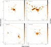 |
Fig. A.1 Continuum emission maps (continued). |
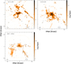 |
Fig. A.1 Continuum emission maps (continued). |
Appendix B Spectral index maps
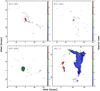 |
Fig. B.1 Spectral index maps (continued from Fig. 4). The ellipses in pink highlight sources automatically flagged due to their spectral index; those in yellow display the sources whose spectral index were further checked manually (see Eq. 2). |
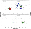 |
Fig. B.1 Spectral index maps (continued). |
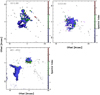 |
Fig. B.1 Spectral index maps (continued). |
References
- Alstott, J., Bullmore, E., & Plenz, D. 2014, PLoS ONE, 9, e85777 [CrossRef] [Google Scholar]
- Alves, J., Lombardi, M., & Lada, C. J. 2007, A&A, 462, L17 [NASA ADS] [CrossRef] [EDP Sciences] [Google Scholar]
- Bastian, N., Covey, K. R., & Meyer, M. R. 2010, ARA&A, 48, 339 [Google Scholar]
- Bonfand, M., Csengeri, T., Bontemps, S., et al. 2024, A&A, 687, A163 [NASA ADS] [CrossRef] [EDP Sciences] [Google Scholar]
- Bonnor, W. B. 1956, MNRAS, 116, 351 [NASA ADS] [CrossRef] [Google Scholar]
- Bontemps, S., Motte, F., Csengeri, T., & Schneider, N. 2010, A&A, 524, A18 [NASA ADS] [CrossRef] [EDP Sciences] [Google Scholar]
- Cheng, Y., Tan, J. C., Liu, M., et al. 2018, ApJ, 853, 160 [NASA ADS] [CrossRef] [Google Scholar]
- Clauset, A., Shalizi, C. R., & Newman, M. E. J. 2009, SIAM Rev., 51, 661 [NASA ADS] [CrossRef] [Google Scholar]
- Csengeri, T., Bontemps, S., Wyrowski, F., et al. 2017, A&A, 600, L10 [NASA ADS] [CrossRef] [EDP Sciences] [Google Scholar]
- Dell’Ova, P., Motte, F., Gusdorf, A., et al. 2024, A&A, 687, A217 [NASA ADS] [CrossRef] [EDP Sciences] [Google Scholar]
- Fiorellino, E., Elia, D., André, P., et al. 2021, MNRAS, 500, 4257 [Google Scholar]
- Galván-Madrid, R., Díaz-González, D. J., Motte, F., et al. 2024, arXiv e-prints, [arXiv:2407.07359] [Google Scholar]
- Garrod, R. T., Vasyunin, A. I., Semenov, D. A., Wiebe, D. S., & Henning, T. 2009, ApJ, 700, L43 [NASA ADS] [CrossRef] [Google Scholar]
- Ginsburg, A., Goddi, C., Kruijssen, J. M. D., et al. 2017, ApJ, 842, 92 [Google Scholar]
- Ginsburg, A., Csengeri, T., Galván-Madrid, R., et al. 2022, A&A, 662, A9 [NASA ADS] [CrossRef] [EDP Sciences] [Google Scholar]
- Girart, J. M., Fernández-López, M., Li, Z. Y., et al. 2018, ApJ, 856, L27 [CrossRef] [Google Scholar]
- Goddi, C., Ginsburg, A., Maud, L. T., Zhang, Q., & Zapata, L. A. 2020, ApJ, 905, 25 [NASA ADS] [CrossRef] [Google Scholar]
- Hennebelle, P., & Chabrier, G. 2008, ApJ, 684, 395 [Google Scholar]
- Izquierdo, A. F., Galván-Madrid, R., Maud, L. T., et al. 2018, MNRAS, 478, 2505 [NASA ADS] [CrossRef] [Google Scholar]
- Koen, C., & Kondlo, L. 2009, MNRAS, 397, 495 [CrossRef] [Google Scholar]
- Kong, S. 2019, ApJ, 873, 31 [NASA ADS] [CrossRef] [Google Scholar]
- Könyves, V., André, P., Men’shchikov, A., et al. 2010, A&A, 518, L106 [NASA ADS] [CrossRef] [EDP Sciences] [Google Scholar]
- Lin, Y., Csengeri, T., Wyrowski, F., et al. 2019, A&A, 631, A72 [NASA ADS] [CrossRef] [EDP Sciences] [Google Scholar]
- Liu, M., Tan, J. C., Cheng, Y., & Kong, S. 2018, ApJ, 862, 105 [CrossRef] [Google Scholar]
- Louvet, F., Motte, F., Hennebelle, P., et al. 2014, A&A, 570, A15 [NASA ADS] [CrossRef] [EDP Sciences] [Google Scholar]
- Louvet, F., Dougados, C., Cabrit, S., et al. 2018, A&A, 618, A120 [NASA ADS] [CrossRef] [EDP Sciences] [Google Scholar]
- Louvet, F., Hennebelle, P., Men’shchikov, A., et al. 2021, A&A, 653, A157 [NASA ADS] [CrossRef] [EDP Sciences] [Google Scholar]
- Lu, J. R., Do, T., Ghez, A. M., et al. 2013, ApJ, 764, 155 [NASA ADS] [CrossRef] [Google Scholar]
- Marsh, K. A., Whitworth, A. P., & Lomax, O. 2015, MNRAS, 454, 4282 [Google Scholar]
- Men’shchikov, A. 2013, A&A, 560, A63 [Google Scholar]
- Men’shchikov, A. 2017, A&A, 607, A64 [Google Scholar]
- Men’shchikov, A. 2021a, A&A, 654, A78 [NASA ADS] [CrossRef] [EDP Sciences] [Google Scholar]
- Men’shchikov, A. 2021b, A&A, 649, A89 [EDP Sciences] [Google Scholar]
- Men’shchikov, A., André, P., Didelon, P., et al. 2012, A&A, 542, A81 [Google Scholar]
- Molinari, S., Swinyard, B., Bally, J., et al. 2010, PASP, 122, 314 [Google Scholar]
- Molinari, S., Schisano, E., Faustini, F., et al. 2011, A&A, 530, A133 [NASA ADS] [CrossRef] [EDP Sciences] [Google Scholar]
- Moser, E., Liu, M., Tan, J. C., et al. 2020, ApJ, 897, 136 [NASA ADS] [CrossRef] [Google Scholar]
- Motte, F., Andre, P., & Neri, R. 1998, A&A, 336, 150 [NASA ADS] [Google Scholar]
- Motte, F., Zavagno, A., Bontemps, S., et al. 2010, A&A, 518, A77 [Google Scholar]
- Motte, F., Nony, T., Louvet, F., et al. 2018, Nat. Astron., 2, 478 [Google Scholar]
- Motte, F., Bontemps, S., Csengeri, T., et al. 2022, A&A, 662, A8 [NASA ADS] [CrossRef] [EDP Sciences] [Google Scholar]
- Olguin, F. A., Sanhueza, P., Guzmán, A. E., et al. 2021, ApJ, 909, 199 [NASA ADS] [CrossRef] [Google Scholar]
- Olguin, F. A., Sanhueza, P., Ginsburg, A., et al. 2022, ApJ, 929, 68 [NASA ADS] [CrossRef] [Google Scholar]
- Olguin, F. A., Sanhueza, P., Chen, H.-R. V., et al. 2023, ApJ, 959, L31 [NASA ADS] [CrossRef] [Google Scholar]
- O’Neill, T. J., Cosentino, G., Tan, J. C., Cheng, Y., & Liu, M. 2021, ApJ, 916, 45 [NASA ADS] [CrossRef] [Google Scholar]
- Ossenkopf, V., & Henning, T. 1994, A&A, 291, 943 [NASA ADS] [Google Scholar]
- Pillai, T., & Simplifi Team 2023, in American Astronomical Society Meeting Abstracts, 55, 308.03 [NASA ADS] [Google Scholar]
- Pouteau, Y., Motte, F., Nony, T., et al. 2022, A&A, 664, A26 [NASA ADS] [CrossRef] [EDP Sciences] [Google Scholar]
- Salpeter, E. E. 1955, ApJ, 121, 161 [Google Scholar]
- Sanhueza, P., Contreras, Y., Wu, B., et al. 2019, ApJ, 886, 102 [Google Scholar]
- Schneider, F. R. N., Sana, H., Evans, C. J., et al. 2018, Science, 359, 69 [NASA ADS] [CrossRef] [Google Scholar]
- Schuller, F., Menten, K. M., Contreras, Y., et al. 2009, A&A, 504, 415 [NASA ADS] [CrossRef] [EDP Sciences] [Google Scholar]
- Vaillancourt, J. 2016, Characterizing the FIR polarization spectrum in Galactic Clouds, SOFIA Proposal, Cycle 5, ID. 05_0038 [Google Scholar]
One can download the extraction catalogues from both getsf and GExt2D, at the native and smoothed angular resolutions on the website of the ALMA-IMF Large Program (https://www.almaimf.com/), and on CDS in a machine-readable format.
A similar figure showing the sources extracted by both algorithms is accessible on Zenodo.
A similar figure for GExt2D extractions is published on Zenodo.
We illustrate the cumulative complementary SFFs with constant logarithm flux interval. This method introduces a constant weight for each bin, regardless of the number of sources constituting the bin. Therefore, it artificially creates a bias for relatively unpopulated bins. For this reason, we ignored the last ten sources from the fit.
We adopted an uncertainty of 5 K for sources below 20 K.
Bonfand et al. (2024) reported six sources with temperatures estimated at 300±100K. The three additional sources with respect to ours are either classified as free-free contaminated (source W51-E-MF1) or do not match our continuum extractions (sources W51-E-MF2 and W51-IRS2-MF3).
We stress that choosing a 3D oblate core shape (V ∝ a2 × b) has no effect on the boundedness of the cores.
We note that xmin = 1.40 M⊙ corresponds to α = 2.07 ± 0.06, compatible with the a associated with xmin = 1.64 M⊙.
σ refers to a confidence interval of a Gaussian distribution.
All Tables
Resolutions, noise levels, and sources extracted after smoothing to a linear scale of 2700 au.
All Figures
|
Fig. 1 Scatter plots of the source size (black dots) extracted with getsf before (left) and after (right) the maps were smoothed to a homogeneous spatial resolution of 2700 au. The blue triangles display the beam sizes. The orange diamonds display the mean sizes of sources. In the left panel, the y-axis is the linear scale (beam × distance) of the maps in Band 6, and the orange line shows the fit to the mean source size distribution for each field. In the right panel, the orange line shows the mean core size of all 15 protoclusters, and the red crosses illustrate the cores exceeding 25 M⊙. |
| In the text | |
|
Fig. 2 Fifteen ALMA-IMF protoclusters as traced by their continuum emission at 1.3 mm at a matched spatial resolution of 2700 au. The ellipses locate all the cores found by getsf. The name of the field is indicated in the top left corner of each panel, and the beam size is shown in the bottom left corner. For each protocluster, the centre coordinates are those specified in Table 1. We show the remaining fields in Fig. A.1. |
| In the text | |
|
Fig. 3 Source flux distributions for the getsf and GExt2D source extractions. The left panel displays the SFFs of the sources extracted by getsf in grey and by GExt2D in blue. The vertical blue and grey lines indicate the median values for each source catalogues, which differ by ≃5%. The right panel displays the complementary cumulative SFFs from the getsf source extraction (in grey) and from the GExt2D source extraction (in blue). The grey and blue lines display the best fits from linear regressions on the complementary cumulative SFFs from the median value at 12 mJy up to the flux at which the number of cores is smaller than 10. The corresponding ζ power-law indexes are indicated in the top right corner. |
| In the text | |
|
Fig. 4 Maps of the spectral index in the 15 ALMA-IMF fields. We chose the colours such that red traces dust thermal emission, blue traces free-free emission, and green likely traces a mixture of dust and free-free emissions. The maps display the spectral index value only where the 3 mm intensity exceeds 3 σ. The black ellipses display the sources extracted by getsf. We show the remaining fields in Fig. B.1. |
| In the text | |
|
Fig. 5 Convergence towards the best fit of a power law through the MLE and KSD method for the global getsf bound core catalogue without the free-free sources. The left vertical dashed line highlights the first minimal KSD (in blue), occurring at xmin = 1.40 M⊙. The right vertical dashed line highlights the completeness limits at xmin = 1.64 M⊙. The orange curve shows the exponent of the power-law fit of the high-mass tail of the CMF as a function of xmin. |
| In the text | |
|
Fig. 6 The grey curves show the complementary cumulative CMFs of the 103 core samples obtained by including flux measurement uncertainties, varying core temperatures, and applying opacity index variations on a per-regions basis (see Sect. 5.2.2), overlaid with the average fit by a power law (in blue) and the best fit with a power-law index 2.35 (in red). |
| In the text | |
|
Fig. 7 Power-law exponents α retrieved when sorting 330 cores from a synthetic core sample whose CMF has a power-law exponent of 1.97 (in blue) and 2.35 (in orange). |
| In the text | |
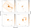 |
Fig. A.1 Continuum emission maps (continued from Fig. 2). |
| In the text | |
|
Fig. A.1 Continuum emission maps (continued). |
| In the text | |
|
Fig. A.1 Continuum emission maps (continued). |
| In the text | |
|
Fig. B.1 Spectral index maps (continued from Fig. 4). The ellipses in pink highlight sources automatically flagged due to their spectral index; those in yellow display the sources whose spectral index were further checked manually (see Eq. 2). |
| In the text | |
|
Fig. B.1 Spectral index maps (continued). |
| In the text | |
|
Fig. B.1 Spectral index maps (continued). |
| In the text | |
Current usage metrics show cumulative count of Article Views (full-text article views including HTML views, PDF and ePub downloads, according to the available data) and Abstracts Views on Vision4Press platform.
Data correspond to usage on the plateform after 2015. The current usage metrics is available 48-96 hours after online publication and is updated daily on week days.
Initial download of the metrics may take a while.