| Issue |
A&A
Volume 673, May 2023
|
|
|---|---|---|
| Article Number | A22 | |
| Number of page(s) | 15 | |
| Section | Stellar structure and evolution | |
| DOI | https://doi.org/10.1051/0004-6361/202245670 | |
| Published online | 26 April 2023 | |
Tachocline Alfvén waves manifested in stellar activity
Space Research Institute (IWF), Austrian Academy of Sciences, Schmiedlstrasse 6, 8042 Graz, Austria
e-mail: maxim.khodachenko@oeaw.ac.at
Received:
12
December
2022
Accepted:
18
March
2023
Context. The short-time (< 700 days) periodicities of both the stellar and solar activity that controls space weather are usually are discussed as manifestations of Rossby modes in tachoclines. Various interpretations of this phenomenon that have been proposed, in particular for the Sun, can be verified by considering the broad population of nonsolar-type stars.
Aims. We look for surface stellar activity features, drifting in longitude, and compare their drift rates with those predicted for different low-frequency waves in stellar photospheres and tachoclines.
Methods. Analogously to the Hovmöller diagrams in meteorology, we constructed a dynamic diagram of stellar activity pattern (DDSAP) to visualize the rotational variability of the stellar radiation flux as a function of rotation phase and time. We used the high-precision light curves of the fast-rotating main sequence stars, with rotation periods of 0.5 to 4 days, from the Kepler mission database.
Results. We found quasi-periodic drifting lanes (DLs) of various durations and intensities in the DDSAPs for 108 stars. In the course of analysis, we carried out a correction of the stellar rotation periods by nullifying the drifts of the longest-lasing DLs that are presumably related to the long-lived starspot complexes co-rotating with the star. We discovered a clear elongated cluster of the absolute values of the DLs’ drift rates versus the stellar effective temperatures. This cluster cannot be attributed to any accidental contaminations of the light curves or manifestation of waves in the stellar photospheres, because of their extremely short timescales. An approximate equality of the absolute values of positive and negative drift rates of the considered DLs makes it impossible to interpret them in terms of Kelvin and/or magneto-Rossby waves in the stellar tachoclines. It is only global kink-type Alfvénic oscillations of the tachocline as a whole that allow us to interpret the estimated drift rates forming the above-mentioned cluster, as well as the related activity periodicities and turnover times in the convective zones. The corresponding magnetic field strength appears to be about 50 kG, which is approximately in the middle of the range of assumptions discussed in the literature.
Conclusions. Alfvén waves are an important, albeit commonly ignored factor in stellar interiors. Apparently, the global tachocline’s Alfvén waves ought to play a role in triggering emergence of the magnetic flux tubes. Their manifestation in stellar activity opens up a unique way of probing the magnetic field strength in tachoclines of individual stars. Since the investigations of the tachocline waves performed thus far have been based on the shallow-fluid approximation, and also assuming a rigid fixed bottom of the tachocline layer, the global kink-type Alvénic disturbances of the whole tachocline layer have not been considered. The reported observational detection of signatures of such waves, manifested in specific longitude drifts of the stelar surface activity pattern, calls for a more detailed theoretical study.
Key words: stars: activity / starspots / stars: interiors / waves
© The Authors 2023
 Open Access article, published by EDP Sciences, under the terms of the Creative Commons Attribution License (https://creativecommons.org/licenses/by/4.0), which permits unrestricted use, distribution, and reproduction in any medium, provided the original work is properly cited.
This article is published in open access under the Subscribe to Open model. Subscribe to A&A to support open access publication.
1. Introduction
The short-time (≲700 days) cycles of solar and stellar activity are usually interpreted as manifestations of the dynamo-process in stellar interiors, modulated by the HD/MHD waves (e.g., Lou 2000; Cai et al. 2021; Zaqarashvili 2018; Zaqarashvili et al. 2021 and references therein). Such a hypothesis equates activity periods with the periods of certain wave modes within an assumption of particular magnetic field strength in the tachocline. Zaqarashvili et al. (2010) discussed several possible explanations of periodicity of the solar activity, involving inertial g- and Rossby (r-) waves, which are supposed to modulate the magnetic flux emergence. Further developments of this approach have involved fast magneto-Rossby waves (Gachechiladze et al. 2019), magneto-Rossby-gravity, and magneto-inertia-gravity (Zaqarashvili 2018) waves. All these interpretations of the solar activity periods can be verified by a consideration of the broad family of nonsolar stars.
In fact, various MHD waves could be manifested in the stellar activity pattern via specific fingerprints. In particular, different modes and their harmonics have different phase velocities. At the same time, as commonly assumed, all these waves can modulate the emergence of magnetic flux (e.g., Zaqarashvili et al. 2010, 2021). Therefore, the longitude drifts in the stellar activity pattern could indicate its trigger wave type and specific features. Such a drift-based approach was applied only once in an analysis of solar coronal activity (McIntosh et al. 2017), whereas studies of stellar activity have been focused only on the determination of temporal characteristics, namely, periods (e.g., Vida et al. 2014; Arkhypov & Khodachenko 2021; Gurgenashvili et al. 2022), whereas spatial and directional aspects of waves propagation were ignored.
A fully elaborated asteroseismic wave diagnostic technique exists, which can be applied to the upper main sequence B, A, and F stars, by addressing the p-, g-, and r-modes (Saio et al. 2018), however, internal Alfvén waves in stars are still poorly studied. At the same time, it is worth mentioning, that the Alfvén waves in tachocline have been investigated for the Sun in terms of a factor that modifies the transport properties (viscosity and diffusivity) of a turbulent medium (Leprovost & Kim 2007), among other possible modes (e.g., shear, Rossby). These studies have shown them to act as a favorable influencer on the magnetic field diffusion (unlike the Rossby modes).
Moreover, we note that the large-scale Alfvénic disturbances of the tachocline layer as a whole ought to affect the emergence of magnetic flux and be manifested in the drifts of the stellar activity pattern. Thus, they could be used as a unique instrument to quantify the internal magnetic field strength in a star. In that respect, here we present a first detailed and extensive study of the longitude drifts of the stellar activity pattern for a sufficiently large set of the main sequence M, K, G, and late F stars.
The paper is structured as follows. In Sect. 2, we specify the analyzed dataset and explain the basic procedures of data processing. In Sect. 3, we discuss the major peculiarities of the dynamical stellar activity pattern found. Section 4 considers various wave-based interpretations of the discovered modulations and drifts of the stellar activity pattern, along with a justification of their relation to the kink-type Alfvén waves in the stellar tachoclines. Section 5 discusses the ways in which the tachocline Alfvén waves could affect the distribution and longitudinal drifts of the stellar surface activity features, while outlining several physical mechanisms that could lead to excitation of the kink-type Alfvén waves in the tachocline. In Sect. 6, we compare the timescale of the detected tachocline Alfvén waves with the periods of Rieger-type cycles of stellar activity and the stellar deep convection turnover time. Here, we also point to a possible interrelation of these phenomena. Section 7 provides the conclusions and summarizes our findings. The appendix contains tables listing all the objects of the analyzed dataset, including their parameters and features of the dynamic activity pattern.
2. Dataset and method
As an input dataset, we used the high-precision light curves of the main sequence stars with a well-pronounced rotational variability from the Kepler mission database1. This set of objects was already considered in Arkhypov et al. (2016). For the acceptable time resolution of the varying longitude distribution (i.e., phase) of the stellar surface activity pattern, we selected a subset of stars with the shortest rotational periods of 0.5 < Prot < 4 days, according to the catalogs of Nielsen et al. (2013) and McQuillan et al. (2014). Additionally, the giant and sub-giant stars were excluded, if their surface gravity logarithm value in the Mikulski Archive for Space Telescopes (MAST)2 was log(g[cm s−2]) ≤ 4.0 and less then 0.2 dex from the main sequence stars’ values, defined according to the stellar models of fast rotators in Amard et al. (2019), which we discuss further later in this paper. Altogether, we processed and analyzed about four hundred light curves.
Our method is based on the analysis of rotational modulation of the stellar radiation flux, F, which reflects the distribution of the stellar surface activity features (spots and facula) over the longitude. The used public available stellar light curves (PDCSAP_FLUX) from the Kepler mission archive1 were already preprocessed to correct for the instrumental and environmental effects. To exclude the residual, non-rotational variability of F, we calculated the fluctuation, ΔFn, of the normalized flux:
where t is the running time of the radiation flux counting and ⟨F(t)⟩ is the flux averaged over one stellar rotation period, namely, within the sliding time window of t − 0.5Prot < t < t + 0.5Prot. For every count of ΔFn(t), the rotational phase ϕ is found as follows:
![$$ \begin{aligned} \phi (t) = 2 \pi \left[ \frac{t}{P_{\text{rot}}} - \text{ int} \left( \frac{t}{P_{\text{rot}}} \right) \right]. \end{aligned} $$](/articles/aa/full_html/2023/05/aa45670-22/aa45670-22-eq2.gif)
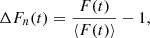
Analogously to the Hovmöller diagram in meteorology (Hovmöller 1949), also used for the modern analysis of solar activity (Fig. 19 in Zaqarashvili et al. 2021), we constructed a dynamic diagram of stellar activity pattern” (DDSAP), which visualizes the rotational variability of the stellar radiation flux as a function of rotation phase ϕ (ordinate), in other words – longitude, and time, t (abscissa). Figure 1 shows an example of such a diagram for the star KIC 9009514. The varying in time fluctuation of the normalized flux, ΔFn, is coded in the gray color scale, so that instead of traditional light curves (flux value versus time), we deal with the color-coded light curves (colored pixel versus time). The time axis (abscissa) in the DDSAP in Fig. 1 is divided into one-rotation period intervals. For each such interval, we plot along the ordinate the color-coded light curve of the given rotation and repeat it three times. Thus, every column in the DDSAP represents the color-coded one-rotation light curve, namely, the variation of ΔFn over 0 < ϕ < 2π. The triple repetition of the one-period color-coded light curves along ordinate enables the tracking of the drifting in longitude activity pattern features at the time intervals essentially longer than one rotation period. In particular, this ensures the continuity of visualization at the boundaries of the considered one-rotation steps (i.e., at ϕ = 0 and ϕ = 2π). The upper part of Fig. 1 shows the variation of activity index σF, as a sequence of the standard deviation values of ΔFn, calculated for each given one-rotation interval. In the DDSAP in Fig. 1 one can see the dark drifting lanes (DLs) at 250 < t < 1000 days with the positive and negative drifts at 250 < t < 500 and 600 < t < 900, respectively, caused by a presumably starspot region. These drifts might be due to decrease of the latitude of appearance of active regions and their groups, analogously to the solar Maunder butterfly effect. It means that the new spots and activity regions, which determine variation of the total irradiation flux from one rotation to another, consecutively appear in the regions with slightly shorter rotation periods, caused by the stellar differential rotation. This will result in the formation in a DDSAP of DLs with positive and negative drifts, relative to Prot, taken as a basis for the DDSAP construction, during the rise and decay phases of the activity cycle, respectively. Such variations of the spot related rotation period are an attribute of short cycles in the late-type Kepler stars (Vida et al. 2014). Altogether, the starspots’ differential rotation effects would affect the variety of measured drifts in the DDSAPs of the considered stellar set. However, as we go on to show in the subsequent sections, these effects will not be dominant; instead, they will just result in certain dispersion of the measured drift values relative a more prominent trend in the behavior of active longitudes caused by wave-related phenomena.
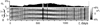 |
Fig. 1. Dynamic diagram of stellar activity pattern (DDSAP) for the star KIC 9009514 with an effective temperature of T = 4569 (according to MAST) and Prot = 1.211 days (according to Nielsen et al. 2013), which shows a typical activity cycle. The accompanying upper plot presents the varying activity index σF, as a sequence of the standard deviations of ΔFn, calculated for each given one-rotation interval. The vertical black bands and strips as well as the black dots in the DDSAP are caused by gaps in photometric data. |
The effects of rotational phase and amplitude in the DDSAPs are naturally separated, as different characteristics of the considered drifting lanes (DLs). In particular, the dark and light colors along the diagram ordinate (i.e., along each vertical one-rotation column) correspond to the maxima and minima of the radiation flux (i.e., amplitude) during the given rotation; whereas the shift of these dark and light features (seen for the series of several consecutive one-rotation columns, i.e., along the diagram abscissa) reflects the longitudinal drift of the corresponding surface activity sources (i.e., the change of their rotational phase from one rotation period to another). The variation of amplitude of the flux fluctuation over the time intervals longer than rotation period, of course, might take place. However, this variation would modulate the contrast of DLs in the DDSAP, but not the rates of their drift D = ∂ϕ/∂t ≡ Δϕ/Δt, defined at the corresponding intervals Δϕ and Δt of their existence. In the reported study, we check possible association of these drifts with the signatures of different MHD waves running in the stellar interiors. The phase and amplitude effects cannot be separated only in the special cases of standing waves and/or opposite propagating similar waves, manifested in the DDSAPs of some stars as the regular modulation patterns built of similar DLs with opposite drifts (discussed below). Such cases were excluded from our study of the drifting activity longitudes in Sect. 6.
It is also worth mentioning that the drifts’ detection capability of the DDSAP method is limited by the way how the DDSAPs are constructed. The limitation is related with the stellar rotation period Prot, which determines the “sampling cadence” of the DDSAP and, therefore, its temporal resolution. This means that only drifts with the rates D < Dcrit = π/Prot can be seen in the DDSAP. In the case of considered fast-rotating stars, all the major surface and interior wave modes which might affect the drifting longitudes of the surface activity pattern appear within the resolution range of the DDSAPs. At the same time, for the more slowly rotating stars, some important wave phenomena may end up beyond the detection capacity of the method; as, for example, in the case of the Sun with Dcrit ≈ 0.11 rad/day.
For the control of correctness of the used stellar rotation period Prot value, the Lomb-Scargle periodograms (Carpintero 2021) were constructed. Figure 2 shows an example of such periodograms, prepared for the same star, KIC 9009514, as in Fig. 1. We can see a clear correspondence between the periodogram peak and the rotation period value Prot from Nielsen et al. (2013), marked with a vertical dotted line in Fig. 2.
 |
Fig. 2. Lomb-Scargle periodogram constructed for the same star, KIC 9009514, as in Fig. 1. The vertical dotted line marks the value of Prot = 1.211 days, provided in Nielsen et al. (2013). The periodogram running value SL − S is calculated with ΔFn, according to Eq. (23) in Carpintero (2021). The value of ⟨F(t)⟩, used in Eq. (1) is smoothed over a widened sliding time-window t − 3Prot < t < t + 3Prot, which also enables the detection of possible parasitic periodicities at timescales of < 6Prot. |
However, the automatically measured catalogue values of Prot (e.g., in Nielsen et al. 2013; or McQuillan et al. 2014) sometimes appear displaced relative to the periodograms’ peaks, whereas the periodograms themselves, for some stars, do not always include any clearly pronounced rotational maxima. To deal with a possible inaccuracy of the applied Prot when the catalogues and periodograms give contradicting values, we performed a correction of Prot on the basis of the reference drift rates Dref = Δϕ/Δt, defined for the clearly pronounced DLs over Δϕ and Δt with the longest lifetimes, Δt, as those in the DDSAP in Fig. 1. Since these dominating DLs are caused by the largest starspots, anchored in the deep layers of convective zone, and rotating with the whole star, they can be used as a reference frame in our drift analysis of other more tiny, or shorter, dynamic features of the stellar activity pattern, manifested in the diagrams. Correspondingly, the measured drift rates Dobs were corrected as follows: D = Dobs − Dref, to obtain the drift rate values, D, used in further analysis and to correct the stellar rotation periods, Pcor = Prot[1 − DrefProt/(2π)], so that the mean longitudinal drifts of the longest DLs, in other words, those of the longest-lived starspot complexes are nullified.
Altogether, the quasi-periodic DLs, which appear to be promising candidates for wave modulations of the stellar activity pattern, were found in the DDSAPs of 79 stars (see Table A.1). Every such case was investigated in detail to measure manually the reference drift rates Dref, based on the longest DLs, as well as the drifts (positive and/or negative) of other DLs, present in the DDSAPs, that are shorter in time and sometimes finer. These secondary drifts were defined separately for various parts of each DDSAP and after correction with respect to Dref were listed in Table A.1 as D1 and D2, of which the first one stays for the smaller corrected drift rate of two. Additionally, 29 cases from the initially considered set of objects, for which the calculation of reference drift Dref was impossible due to specifics of the revealed in the DDSAPs activity patterns (discussed below), are listed in Tables A.2 and A.3. Figure 3 shows the distribution of all stars from Tables A.1–A.3 over the surface gravity logarithm log(g) and effective temperature T, which could be treated as an analog of the HR diagram. We can see a clear clustering of the finally considered stellar subsets around the theoretical main sequence line, constructed using stellar models of fast rotators (Amard et al. 2019) for objects with maximal surface gravity at a given mass.
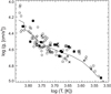 |
Fig. 3. Analog of the HR diagram for the stellar sub-sets from Table A.1 (open squares for positive, and rhombi for negatives drift rates, respectively), Table A.2 (crosses), and Table A.3 (solid squares). The solid line depicts the main sequence, obtained using stellar models of fast rotators (Amard et al. 2019) with maximal surface gravity log(g). |
3. Phenomenology of drifting patterns in the activity diagrams
Figure 4 shows the typical patterns of activity in the DDSAPs constructed with the highest resolution in the (ϕ, t) parameter space. In particular, we can see in Fig. 4a, the relatively long-lasting DLs, caused by the Rieger-type cycles with typical periods from 100 to 200 days, and the signatures of a simple dynamo cycle similar to those in Fig. 1. In Fig. 4b, the analogous cyclic activity pattern with the DLs is modulated by the wave-like processes, manifested as shorter and faster-drifting DLs with a positive drift. We note that the modulation amplitude, as seen in the dynamics of activity index, σF, is maximal during the Rieger-type cycle maxima and minimal in between. This feature allows us to rule out a possible hypothetic contamination of the light curve by an unresolved companion in a binary system, since the external additive contribution of the companion should not depend on the phase of the stellar Rieger-type cycle. Another argument against the contamination hypothesis consists in the coexistence in Fig. 4c of the positively and negatively drifting DLs with the approximately equal absolute drift rates. The number of such cases, listed in Table A.2, shows that this phenomenon is unlikely to be related to the occasional coincidences of independent rotations in the multiple stellar systems.
 |
Fig. 4. Examples of typical patterns of activity in the (ϕ, t) parameter space of the DDSAPs, constructed for: (a) KIC 9119108 with T = 4944 K and Prot = 0.64284 days; (b) KIC 8621739 with T = 6198 K and Prot = 0.922 days; (c) KIC 7915824 with T = 6230 K and Prot = 0.740 days; (d) KIC 8144578 with T = 6642 K and Prot = 0.593 days. The effective temperatures, T, are set according to MAST and rotation periods, Prot, are taken from McQuillan et al. (2014). |
An alternative interpretation of the activity pattern visualized in Fig. 4c is two counter-propagating surface waves running simultaneously on a single star. In the case when these waves are similar to each other (i.e., equal wavelengths, periods, and amplitudes), a standing-wave-like pattern with a regular node-antinode structure is formed in the DDSAP. The transitions from patterns with the drifting and intersecting lanes in Fig. 4d, at 250 < t < 350 days and 1170 < t < 1300 days, respectively, to the regular standing-wave-like patterns (e.g., at 740 < t < 1025 days) confirm the suggested wave interpretation of the observed activity pattern behavior. The standing wave-like pattern in Fig. 4d, lasting over ∼300 days, is too long for the starspots beating, manifested as an oscillation of amplitude of rotational variability. This effect takes place in the case of two spots (or active regions) moving with different rotational periods at different latitudes. It could, in principle, produce similar features in the DDSAPs, but the spots’ lifetime is usually much shorter (∼20 days, see, e.g., the panel for 6400 < T < 6800 K in Fig. 16 in Basri et al. 2022). Moreover, the standing wave-like patterns could sometimes exist even longer, for instance, over ∼700 days and ∼1000 days in the cases of KIC 3239219 and KIC 1570924, respectively.
As a complement to Fig. 4, we show in Fig. 5 the diversity of DL drifts, which range from the fast (|D|∼1 rad s−1), in Fig. 5a,b, through the medium (0.02 ≲ |D|≲0.5 rad s−1), in Fig. 5c,d, up to the slow (|D|≲0.02 rad s−1), in Fig. 5e, values. The periodicity of DLs is a characteristic attribute, indicating their wave-like nature.
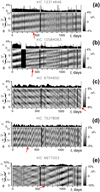 |
Fig. 5. Examples of different types of DLs in the (ϕ, t) parameter space of the DDSAPs, constructed for: (a) KIC 12314646 with T = 3444 K and Prot = 2.725 days (according to McQuillan et al. 2014; b) KIC 10584063 with T = 3323 K and Prot = 1.602 days (according to McQuillan et al. 2014; c) KIC 6794650 with T = 5370 K and Prot = 1.796 days (according to Nielsen et al. 2013); (d) KIC 7537808 with T = 5430 K and Prot = 2.388 days (according to Nielsen et al. 2013); (e) KIC 6677003 with T = 5246 K and Prot = 3.177 days (according to Nielsen et al. 2013). The effective temperatures, T, are taken from MAST. Red arrows mark various drift directions. |
The estimates of drift rates (provided in Table A.1) are distributed versus T in a way that is not random, as it might be expected for the contamination hypothesis, but they are clustered in a kind of sequence, as seen in Fig. 6. For log(T)≳3.65, this sequence includes the positive and negative drifts, which are relatively close to each other in absolute value |D|, whereas for log(T) < 3.65, there are mostly positive drifts present. This effect is also difficult to interpret in terms of the contamination hypothesis, because it would require rather strange restrictions for the temperature and orbital lockings of the binary system components.
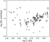 |
Fig. 6. Distribution of the drift rate estimates, D1 and D2, from Table A.1 versus the log of the stellar effective temperature, T. The positive and negative drifts are marked with open squares and open rhombi, respectively. |
Moreover, the Kepler and Gaia catalogs of binary systems (Kirk et al. 2016; Gaia Collaboration 2023) do not confirm any significant peculiarities in the distribution of stellar orbital periods in the considered typical range from 0.5 to 4 days. Therefore, the contamination hypothesis for the explanation of the discovered clustering of the stellar activity pattern drift rates in Fig. 6 does not appear convincing, and the wave-based interpretation of the phenomenon appears more realistic. The latter is considered in detail in the follow-up analysis.
4. Revealing the modulating wave type in the stellar activity pattern
To compare the measured drift rates D of the DLs in the DDSAPs with the theoretically predicted manifestations of waves in the stellar surface (photospheric) activity phenomena, we converted them to the phase velocities of waves as follows:

where R* is the stellar radius according to MAST2.
Figure 7a,b shows the calculated with Eq. (3) distributions of the absolute values of phase velocity Vph of waves, modulating the stellar activity pattern, versus the log of the stellar effective temperature T in the cases of positive (Fig. 7a), that is, retrograde wave propagation with respect to the stellar rotation, and negative (Fig. 7b), that is, prograde wave propagation with respect to the stellar rotation (drifts D1 and/or D2 from Table A.1). The theoretical predictions (superimposed in Fig. 7a,b) for the different waves in photosphere (labeled curves) were calculated using the corresponding dispersion equations from Lou (2000) within the shallow-fluid approximation, taking into account that Vph = ω/k, where ω is the wave cyclic frequency, k = m/R* is the wave vector, and m = (2πR*)/λ is an azimuthal number of the wave with the length λ, propagating over the stellar surface. The used stellar parameters, such as effective temperature, T, and surface gravity, g, for the given radius, R*, and mass, were extracted from the model grid for the fast rotators (Amard et al. 2019). For that purpose, we took the models with the maximal surface gravity at the given stellar mass and quasi-solar metallicity, Z = 0.013 (i.e., the main sequence stars were considered). The shallow-fluid gravity-wave speed  was calculated, using the gravitational scale height at the surface
  , where kb is Boltzmann’s constant, and
  stays for the overall mean particle weight, defined as follows:
 |
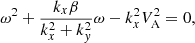
Fig. 7. Distributions of the absolute values of phase velocity Vph of waves, modulating the stellar activity pattern, estimated with Eq. (3) for the drift rates, D1 and D2, from Table A.1, versus the log of the stellar effective temperature T. (a) the positive drifts (squares); (b) the negative drifts (rhombi). The labeled curves depict the theoretic predictions for the different waves in photospheres of the main sequence stars, according to the dispersion relations from Lou (2000) and stellar parameters from the models of fast rotators in Amard et al. (2019) with maximal surface gravity. Panel (c) shows the range of the actual values (grey) of the small parameter βo = 2Ω/R*, used for the solving of the dispersion equations in β-plane approximation for the considered shallow-fluid wave modes. |
Here mp is the proton mass; X ≈ 0.72, Y ≈ 0.26, and Z ≈ 0.02 are the mass fractions for H, He, and metals in the solar-type composition stars, respectively (Owocki 2019). Figure 7c shows the corresponding range of actual values of the small parameter βo = 2Ω/R* ≪ 1, which ensures the applicability of the so-called β-plane approximation of the dispersion equation (Rossby et al. 1939; Lou 2000) for the considered here shallow-fluid wave modes. Here (and further on in this work), Ω = 2π/Prot is the stellar rotation angular velocity, which is calculated for all considered stars with 0.5 < Prot < 4 days in the analyzed set. We note that we do not consider here the magneto-waves in photospheres, since the magnetic field of active regions is very complex. Such a rather chaotic field cannot be related with the global, quasi-linear drifts of the active longitudes, manifested as DLs in the DDSAPs.
We can see in Fig. 7a that only a few cases in the considered set of stars with the maximal values of the estimated |Vph| can be associated with the gravity (g-modes) or equatorially trapped Rossby waves in the stellar photospheres. At the same time, g-modes are a well-known driver of the γ Dor type variability in F and A stars of the main sequence (Kaye et al. 1999). Apparently, a small amount of the fast drifts in Fig. 7a also reveal gravity waves in the cold M-stars. However, the majority of the estimations of |Vph| in Fig. 7a, and especially those in Fig. 7b, are located essentially below the predicted values for the photospheric waves. This discrepancy points to the likelihood of a deeper location of the waves, which are responsible for the drifting features of the stellar activity pattern discussed here. The next physically relevant layer in that respect is the stellar tachocline, appeared at the bottom boundary of the convective zone (Charbonneau et al. 1999) at the radial distance, Rt, from the stellar center. This region is traditionally considered in the context of possible modulations of the solar activity by various wave modes (e.g., Gachechiladze et al. 2019; Zaqarashvili et al. 2010, 2021 and therein). Therefore, we naturally look at the tachocline region as well.
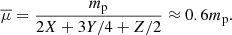
In view of the said above, Fig. 8a,b shows the distributions of the absolute values of the recalculated for the stellar tachoclines phase velocity of waves,

 |
Fig. 8. Distributions of the tachocline version of the absolute values of phase velocity Vt of waves, modulating the stellar activity pattern, estimated with Eq. (5) for the drift rates D1 and D2 from Table A.1, versus the log of the stellar effective temperature T. (a) the negative drifts (rhombi); (b) the positive drifts (squares). The tachocline radius Rt, as well as other stellar parameters, are taken from the models of the main sequence fast rotators in Amard et al. (2019) with maximal surface gravity. The labeled curves depict the theoretic predictions for the different waves in tachoclines of the main sequence stars, according to the dispersion relations from Zaqarashvili (2018) and Gachechiladze et al. (2019), taking the most observable lowest-number spherical harmonics (n = m = 1). The numbers near the theoretical curves for the equatorial magneto-Kelvin waves in panel (a) indicate the assumed thicknesses of the tachocline in units of R*. Blue lines of the Alfvén velocity VA in panels (a) and (b) are calculated for B = 50 kG (solid), B = 100 kG (dashed, upper), and B = 25 kG (dashed, lower). Panel (c) shows the range of the actual values (grey) of the small parameter β = VA/(ΩRt)≪1 used for the solving of the dispersion equations for the considered wave modes in the shallow-fluid approximation. |
versus the log of the stellar effective temperature, T, in the cases of negative (Fig. 8a) and positive (Fig. 8b) drifts D1 and/or D2 from Table A.1. The radii of the stellar tachoclines, Rt, used here were taken from the stellar model grid (Amard et al. 2019) as the radii of the bottom boundaries of the convective zones of the main sequence stars, identified as objects with the maximal surface gravity at the given mass. These models were also used to obtain, along with other stellar parameters, the density of plasma ρ in the tachoclines, needed for the calculation of the local Alfvén velocity,  , where B is the value of the toroidal magnetic field in the tachocline.
We can see in Fig. 8a that the majority of the estimated values of |Vt| for the negative (prograde wave propagation) drifts are clustered around the lines of Alfvén velocity VA, calculated for B = 50 kG (solid line), B = 100 kG (dashed upper line), and B = 25 kG (dashed lower line). The range of the magnetic field values 25 ≤ B ≤ 100 kG, used here, is on the same order of magnitude as that proposed for the solar tachocline, for instance, 7 kG–50 kG (in Gachechiladze et al. 2019); 10 kG–15 kG (in Gurgenashvili et al. 2021); 7.5 kG–30 kG (in Teruya et al. 2022); B ≥ 100 kG (in Zaqarashvili et al. 2010). Figure 8b, which shows the distribution of the |Vt| estimates in the case of positive (retrograde wave propagation) drifts, also reveals their clustering around the same lines of Alfvén velocity.
The discovered correlation between the distributions of the Vt estimates and the VA lines in Fig. 8a,b obviously cannot be a result of the stellar light curves contamination, since the external factors (e.g., interference from companions) does not depend on the stellar interior parameters, such as ρ and B, used for the calculation of VA).
It is also important that the Alfvénic region in Fig. 8a,b appears sufficiently far from the range of predicted values for other modes, considered in the shallow-fluid approximation, controlled by the small parameter β = VA/(ΩRt)≪1, which actual range is shown in Fig. 8c. In particular, the prograde equatorially trapped magneto-Kelvin waves in Fig. 8a, have according to Eq. (50) in Zaqarashvili (2018), the phase velocity of  . The gravity acceleration in tachocline gt, used here, is again defined from the stellar models (Amard et al. 2019), whereas the unknown thickness of tachocline layer Ht is taken 0.001R*, 0.01R*, and 0.1R*, having in mind that the solar value is 0.04RSun (Charbonneau et al. 1999). In fact, the generic range of magneto-Kelvin waves is located even at higher velocities,
  , which is not shown in Fig. 8a, as well as the range of magneto-inertia-gravity waves (see e.g., Fig. 1 in Zaqarashvili 2018).
The prograde slow magneto-Rossby waves, according to Eq. (36) in Gachechiladze et al. (2019), have a phase velocity of  . Correspondingly, the range of slow magneto-Rossby waves in Fig. 8a was calculated, using the same values of VA, as those, which define the Alfvénic region, whereas Ω was calculated for all stars in the considered set. Analogously, the range of retrograde fast magneto-Rossby waves, shown in Fig. 8b, is defined by phase velocity 2ΩRt/[n(n + 1)], according to Eq. (35) in Gachechiladze et al. (2019), with the zonal number n = 1, which corresponds to the modulation, most easily detectable in Kepler integral photometry. In fact, this range of fast magneto-Rossby waves overlaps with the range of the equatorial fast magneto-Rossby waves (Eq. (40) in Zaqarashvili 2018), which is not shown in Fig. 8b. Although some outliers in Fig. 8b could be associated with the fast magneto-Rossby waves with zonal numbers n > 1, the Alfvén waves remain the best candidates in the majority of cases for the interpretation of wave driver, which modulates the stellar activity pattern.
Generally speaking, there is a question regarding the type of Alfvénic disturbances in the tachocline, which result the observed drifts of the stellar activity pattern and their relation with other MHD modes, such as Rossby waves detected in the Sun and stars (Zaqarashvili et al. 2021). We go on to consider the dispersion equation for the low-frequency branch of MHD waves in a thin rotating spherical layer of conductive fluid, obtained within the shallow-fluid approximation in the form of Eq. (17) from Zaqarashvili et al. (2007), as follows:
where ω is the cyclic frequency of the wave, kx and ky are the projections of the wave vector in the longitude and latitude directions, respectively, and  is the rate of Coriolis parameter change with the latitude Θ. The general solution of this biquadratic equation yields the fast and slow magneto-Rossby waves. In the case when the second term in Eq. (6) is negligible, it turns to the Alfvén wave equation: ω = ±kxVA. The smallness of the second term can be achieved either for the large values of the wave vector, kx, (short wavelength approximation) or for the high Alfvénic speeds, VA, (strong magnetic field), as well as for the small values of β, realized in close vicinity of the stellar poles. Such an asymptotic character of the Alfvénic mode, according to Eq. (6), reflects the condition of a so-called Alfvén limit with the convergence of slow and fast magneto-Rossby modes to the Alfvén wave, achieved in the shallow-fluid approximation (e.g., Zaqarashvili et al. 2007, 2021; Zaqarashvili 2018). This means, in particular, that the simultaneous existence of the Alfvén and magneto-Rossby waves in the rotating liquid conductive spherical shell, which resembles the stellar tachocline, is impossible within the applied assumptions. At the same time, the theoretical curves in Fig. 8, calculated according to the solutions provided in Gachechiladze et al. (2019) and Zaqarashvili (2018), show that the convergence of slow and fast magneto-Rossby modes to the Alfvén wave (i.e., Alfvén limit) could, in principle, take place in the hottest stars (T > 6600 K) from our stellar set. However, for the majority of the considered objects this is not the case. This means that the tachocline Alfvén waves manifested in the majority of colder stars in the considered set of fast rotators, which form a pronounced cluster of the empirical estimates in the Alfvénic region in Fig. 8a,b, are not the result of Alfvén limit effect. They have another nature, overlooked in the above-mentioned simple analytical models.
In that respect, it is worth recalling that the theoretical investigations of the tachocline waves which we refer to here, besides the previously mentioned shallow-fluid approximation, assume a rigid (fixed) bottom of the tachocline’s layer and a free upper boundary (e.g., Zaqarashvili et al. 2007). As a result, only oscillations of the tachocline’s thickness, or just flat horizontal motions (e.g., Dikpati et al. 2020) are considered. However, in reality there is no a physical reason, which might prohibit a non-rigidness of the tachocline’s bottom. Correspondingly, the kink-type displacements of the tachocline as a whole (without change in its thickness) should be possible. This kind of a kink-type Alvénic wave in the tachocline layer was excluded from the theoretical analysis, because of the above mentioned limiting assumptions. It is worth noting that the global kink-type Alfvénic oscillations of the stellar tachocline can co-exist with the magneto-Rossby waves in it, regardless of the Alfvén limit condition. Altogether, this view opens up a way of interpreting the observationally discovered Alfvénic region in Fig. 8a,b that is related to the drifting activity longitudes as a manifestation of the global kink-type Alfvén waves running in the stellar tachoclines. The shallow-fluid approximation is inappropriate for the explanation of this phenomenon. The conditions of co-existence of particular wave modes in the tachoclines of different stars (e.g., fast or slow rotators, etc.) and their detectability are a subject for a special follow-up theoretical investigation, which is beyond the scope of the present paper.
5. Phenomenon scenarios and manifestations
Speaking about the way how the kink-type Alfvénic oscillations in the stellar tachoclines could be manifested in the drifting surface activity phenomena, we note that the tachocline’s magnetic field has a dominating azimuthal (toroidal) component. This means that the considered kink-type Alfvén waves propagate along the tachocline and not towards the stellar surface. At the same time, the kink-type Alfvénic disturbances of the tachocline layer should affect the emergence of the kink unstable magnetic flux tubes (e.g., those simulated in Fan et al. 1998 and in Abbett & Fisher 2000), appearing not only a trigger for this process in the bottom of the convection zone, but also a modulating factor for the drifting emergence longitude. Therefore, the emerging magnetic flux and the related distribution of the surface activity regions should carry the fingerprints of the confined kink-type Alfvénic oscillations in the tachocline. This scenario, in particular, seems realistic for the explanation of DLs with medium (0.02 ≲ |D|≲0.5 rad s−1) drift rates in the DDSAPs, as in the case of those in Fig. 5c,d.
As to the possible scenarios that can lead to the excitation of the kink-type of Alfvén waves in the tachocline, the velocity shear (which appears a typical attribute of the tachoclines) might play an important role. In particular, a periodic shear flow of a viscose and resistive fluid, along with the usual Kelvin-Helmholtz instability, effectively generates for any nonzero magnetic field the resistively unstable Alfvén waves, due to so-called Alfvénic Dubrulle-Frisch instability (Fraser et al. 2022). Another possible mechanism of generation of Alfvén waves in the tachocline, which neighbors the bottom of convective zone, might be stellar convection. Vertical disturbances of the magnetized tachocline layer, caused by the convection, could propagate as kink-type Alfvénic disturbances with the phase velocity, VA, along the entire toroidal magnetic field of the tachocline, namely, in the longitudinal prograde and retrograde directions, while triggering the kink instability and emergence of the magnetic tubes.
In the case of counter-propagating (in the prograde and retrograde directions) Alfvén waves from the same source region, an activity pattern with the opposite drifting intersecting DLs, having equal |D|, will be formed in the DDSAP (e.g., as seen in Fig. 4c). When the tachocline circumference contains an integer number of wavelengths and the counter-propagating waves have the same amplitude and frequency, a standing wave-like pattern would appear, similar to that in Fig. 4d.
We note that the scenario traditionally considered with regard to wave-modulated stellar activity deals with the magneto-Rossby waves and it is different from the one we propose here. However, this traditional scenario has a number of fundamental weaknesses in the context of findings reported here, which we briefly address below.
First, the retrograde fast and prograde slow magneto-Rossby waves, which might cause in the DDSAPs the DLs with positive (D ≡ {D1, D2}> 0) and negative (D ≡ {D1, D2}< 0) drift rates, have the difference in phase velocity of more than three orders of magnitude (see Fig. 8a,b). This fact contradicts to the revealed closeness of |D| for the positive and negative drifts, up to approximate equality, seen in Fig. 6 and their clustering within the Alfvénic region in Fig. 8a,b. Moreover, it is impossible to explain, using these magneto-Rossby modes, the stellar activity patterns with opposite drifting intersecting DLs like those in the DDSAP in Fig. 4c as well as the standing-wave-like patterns in Fig. 4d, observed in the stars listed in Tables A.2 and A.3, respectively.
Then, to bring the frequency of fast magneto-Rossby waves to the observed solar periodicities, the waves with high zonal numbers n ≥ 5 (e.g., Gachechiladze et al. 2019) are postulated without physical justification. If such modes indeed exist in our case, then the most easily detectable global Rossby wave with the zonal number n = 1 should be present and seen as well. However, the corresponding regions in Fig. 8a,b are empty.
Next, the negative drifts in Fig. 8a cannot be explained in terms of the retrograde (D > 0) fast magneto-Rossby mode (in principle). At the same time, the prograde (D < 0) slow magneto-Rossby waves have phase velocities that are essentially lower (≲1%) than the values covered by the Alfvénic region, which cannot be related with the positive drifts too.
Finally, there is also a theoretical argumentation, provided in Leprovost & Kim (2007), who have shown that the Alfvén-dominated regime of magnetic field and angular momentum transport prevails over the Rossby-dominated one under the conditions typical for solar tachocline, so that the dynamics of the tachocline is likely to be insensitive to the effect of Rossby waves. However, their study was performed within the assumption of only flat motions, so that vertical kink-type Alfvénic disturbances of the whole tachocline layer were not considered.
Altogether, as pointed out above, all the referred here theoretical studies of the tachocline waves with respect of their possible influence of the stellar and solar surface activity phenomena were performed within the shallow-fluid approximation and assumed a rigid bottom of the tachocline layer. This leads to a complete exclusion from the consideration of the global kink-type Alfvénic oscillations in the tachocline, which (as argued above) can nicely explain the observationally revealed phenomenon of drifting activity longitudes in the reasonably large sample of fast-rotating main sequence stars considered here.
6. Astrophysical applications
The proposed interpretation of the dynamic stellar activity patterns in terms of the Alfvénic disturbances in the tachoclines raises several important issues for the stellar physics. In particular, the scaling of the Rieger-type stellar activity cycles, Pcyc ∝ Prot, in hot main sequence stars, reported in Arkhypov & Khodachenko (2021) was interpreted by the authors as a manifestation of the general Rossby wave scaling ω ∝ Ω, where ω is the cyclic frequency of the wave and Ω stays for the stellar rotation angular velocity. In reality, the average angular velocity Ω of the main sequence stars increases with T (see, e.g., Fig. 5 in Santos et al. 2021) approximately in the same way as VA in the tachocline does. This coincidence suggests a relationship between the activity cycle duration and Alfvén velocity in the tachocline (Fig. 8a,b).
Figure 9 shows the calculated round-star travel periods, Prst = 2π/|D|, of the surface activity features, manifested as DLs in the corresponding DDSAPs of individual stars with D ≡ {D1, D2} from Table A.1, as a function of the log of the stellar effective temperature. In the case of the most easily detectable global wave with the azimuthal number m = 1, which presumably affects the longitudinal drift of the activity features (i.e., the activity longitude), the value of Prst should be equal to the wave period. Thus, it could be compared with the periods Pcyc of the short Rieger-type cycles of stellar activity in the considered stellar sample, measured in Arkhypov et al. (2015) by two independent methods and the approximation of Pcyc(T) as a function of effective temperature provided in that work (see caption of Fig. 15 in Arkhypov et al. 2015). The latter is depicted in Fig. 9 by a green line. We can see that in most cases, we have Prst ≈ Pcyc(T). Moreover, the cluster of Prst estimates, as well as the regression Pcyc(T), coincide well with the region of periods, PA = 2πRt/VA, defined for the global Alfvén waves propagating in the stellar tachoclines. This cluster corresponds, in Fig. 9, to the area between the dashed blue lines. The typical average value of these Alfvénic periods is PA ∼ 150 days.
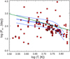 |
Fig. 9. Round-star travel periods, Prst = 2π/|D|, of the surface activity features, manifested as DLs with the positive (squares) and negative (rhombi) drift rates D1 and D2 from Table A.1 versus the log of the stellar effective temperature, T. The blue lines depict the range of periods PA = 2πRt/VA of the global (n = 1) Alfvén waves in the stellar tachoclines with magnetic field B = 50 kG (solid), B = 25 kG (dashed, upper), and B = 100 kG (dashed, bottom). The green line shows the regression for the short Rieger-type cycle periods Pcyc(T), revealed in Arkhypov et al. (2015). |
Altogether, the Rieger-type periodicities of stellar activity play a prominent role in space weather (see, e.g., Table 3 in Zaqarashvili et al. 2021). Hence, the tachocline Alfvén waves, as a possible driver of such cycles, appear an important factor for the stellar-planetary interactions.
Another interesting issue, important for astrophysics, concerns the connection, we notice, between the tachocline Alfvén waves and the stellar convection turnover time τ. Figure 10 summarizes an actual view of τ versus the log of the stellar effective temperature, which includes the empiric estimates (Wright et al. 2011), as well as the numeric calculations (Landin et al. 2010; Amard et al. 2019). As one can see, all values of τ appear within the range of periods  of the tachocline Alfvén waves with the wavelengths Λ equal to the diameter of the stellar laminar convection cell (Dibaj & Kaplan 1976), in other words, when
  , and the magnetic field is B = 25 − 100 kG. Here, Hcz is the thickness of the convective zone, obtained from the models of the main sequence stars (Amard et al. 2019). In particular, the solid blue line in Fig. 10, which shows
  as a function of T in the case of B = 50 kG, practically coincides with the curve of the local turnover time values (red dashed), calculated at the level of half of the mixing length above the base of the convective zone for the main sequence stars of 1 Gyr age, according to the stellar model grid from Landin et al. (2010). Moreover, the same line of
  values is closely approximated by the curve of turnover times (red solid), calculated at the middle (in radius) of convective zone for the main sequence stars (i.e., the maximal surface gravity for the given stellar mass), according to the stellar model grid from Amard et al. (2019). All the empiric estimates of τ in Fig. 10 are distributed between the blue dashed lines which show the range of
  , calculated for the same magnetic field values B = 25 − 100 kG, as those considered above (e.g., in Fig. 8a,b) in our study of the manifestations of the tachocline waves in the drifting stellar activity patterns in the DDSAPs.
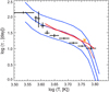 |
Fig. 10. Stellar convection turnover time τ versus the log of the stellar effective temperature, T, according to the empiric estimates in Wright et al. (2011) (black error bar crosses), as well as the numeric models of the main sequence stars in Landin et al. (2010) (red dashed line) and Amard et al. (2019) (red solid line). The yellow asterisk indicates an average estimate of τ for the Sun, based on different sources (see, e.g., Table 2 in Arkhypov et al. 2013). The blue lines depict the range of periods, |

This remarkable accordance between the stellar convection turnover time and the periodicities of the tachocline Alfén waves points at a possible link between them. It indicates that the specific privileged values of the temporal and spatial scales of the stellar convection, used in the mixing length theory (MLT), might be the result of some kind of resonant interaction between of the Alfén waves in the tachocline and the large-scale laminar convection in the stellar convective zone lying above it. We note, in this respect that the stellar models that do not include the tachocline Alfén waves, nevertheless predict the convection timescales close to the wave periods, which is consistent with the physically justified scales of the laminar convection cells. Various manifestations of the laminar convection scale have been found so far in the solar and stellar activity (see e.g., in Arkhypov et al. 2012, 2013, 2016, 2018). Hence, our findings here argue in favor of a possible additional coupling and resonant interaction between the tachocline waves and the stellar convection flows.
7. Conclusions
In the course of the study reported here, the specific and previously unknown longitudinal drifts of the stellar surface activity were discovered by means of the elaborated DDSAP method, applied to the set of 108 main sequence fast-rotating stars (Figs. 4 and 5).
The periodicity of the discovered DLs, as well as the ability of the overall activity pattern in the DDSAPs to transform from the quasi-regular systems of DLs to the regular standing-wave-like patterns with nodes and antinodes, attest to certain wave process(es) involved in the development of the stellar surface activity phenomena and manifested there. These wave processes are manifested also as the short periodic modulations of the main cycle of the stellar activity.
The well-defined elongated cluster of the DLs’ drift rates versus the logarithm of the stellar effective temperature (Fig. 6) is difficult to interpret as an occasional contamination of the stellar light curves. The performed analysis of the measured drift rates excludes their origin as a manifestation of the waves in the photosphere affecting the surface activity, because of the too short timescales of the photospheric waves. Nevertheless, the fast-drifting DLs with |D|∼1 rad s−1 still can be associated with the gravity waves (g-mode) in the photospheres of the main sequence M-F stars.
It is found that the cluster of the drift rate values in Fig. 6 agrees well with the range of Alfvén velocity in the stellar tachocline, located at the bottom of the convective zone (Fig. 8a,b). Altogether, Alfvén waves on the stars are not a new subject. They have been often considered with regard of the solar coronal phenomena, solar and stellar wind acceleration and the turbulence-based coronal heating (e.g., Szente et al. 2017; van der Holst et al. 2014), as well as in the context of the dynamical and transport processes in the solar and stellar tachoclines (Zaqarashvili et al. 2007, 2021; Zaqarashvili 2018; Leprovost & Kim 2007; Dikpati et al. 2020). In that respect, the reported observation-based investigations, of the long-term variations of the stellar surface activity pattern on the fast rotators could be considered as an indirect detection of Alfvén waves in the stellar tachoclines, which are manifested in the form of the drifting surface activity longitudes. The presence of the Alfvén wave related drifts of active longitudes in the stars with different effective temperatures (Figs. 6 and 8), including the clod ones, means that the associated with them tachocline Alfvén waves in the majority of the considered objects are not the result of the Alfvén limit effect, discussed in Sect. 4. They have another nature, not yet addressed in the theoretical studies, which traditionally consider the stellar tachocline as a thin rotating spherical layer of the conductive fluid and employ the shallow-fluid approximation (e.g., Zaqarashvili et al. 2007) or consider only flat motions of the tachocline matter (Dikpati et al. 2020), in both cases assuming a rigid bottom of the tachocline layer. The observationally detected Alfvén waves that we report here represent a specific class of the tachocline waves, which correspond the global kink-type disturbances of the whole tachocline layer without change in its thickness. This kind of kink-type Alfvénic disturbances of the tachocline cannot be described within the traditional shallow-fluid approximation. They call for further development and improvement of the corresponding theoretical models.
The Rossby waves, widely discussed in the context of wave-modulated stellar activity, contradict the empirical fact of the approximate equality of the negative and positive drift rates of the surface activity phenomena (revealed with the DDSAP method and visualized in Fig. 6), as well as the intersecting DLs and standing-wave-like patterns, seen in the DDSAPs. This supposes the closeness of the prograde and retrograde phase velocities of the associated waves. At the same time, for the fast (retrograde) and slow (prograde) magneto-Rossby waves, the values of phase velocity are essentially different. There are also other arguments against the Rossby waves hypothesis, as discussed in Sects. 4 and 5.
The round-star travel periods Prst = 2π/|D| of the surface activity longitude, which are manifested as the DLs with positive and negative drift rates, appear in general agreement with the range of periods PA = 2πRt/VA of the global (m = 1) Alfvén wave propagating in stellar tachocline (taking the magnetic field there to be B = 25 − 100 kG). They are rather close to the measured periods of the well-known Rieger-type cycles of the stellar activity (Fig. 9).
Moreover, the timescale  of the tachocline Alfvén waves, where Λ is the size of the stellar laminar convection cell, appears practically the same, as the stellar convection turnover time used in stellar models and MLT (Fig. 10). This remarkable accordance between the deep stellar convection turnover time, operated in MLT and the tachocline Alfén waves points at their possible connection, so that the characteristic temporal and spatial scales of the convection might be the result of an interplay between of the tachocline kink-type Alfén waves and the convective zone lying above.
Although the Alfvén waves appear an essential attribute of the magnetized tachoclines, they still suffer from a lack of attention in studies of stellar interiors. The presence of the velocity shear in a tachocline rises a question regarding the Kelvin−Helmholtz instabilities, in particular, with respect to the resistively unstable Alfvén waves. In contrast to the ordinary Kelvin−Helmholtz mode, which becomes stable in the case of sufficiently strong magnetic field, the resistively unstable Alfvén waves are excited at any non-zero magnetic field (Fraser et al. 2022). In addition, convective motion is another possible driver of the Alfvén waves in a tachocline, which is adjacent to the bottom of the convective zone. The tachocline Alfvén waves could trigger kink instability of the magnetic tubes and modulate their emergence. Therefore, the kink-type Alfvén waves in the tachoclines can be manifested as the drifting longitudes of the emerging magnetic flux in the stellar photospheres – even in spite of the fact that these waves remain confined in the tachocline layer and do not propagate towards the stellar surface. The findings regarding the behavior of DLs in the analyzed stellar DDSAPs reported here provide empirical support for this scenario.
It is also worth noting that the majority of the analyzed DLs in the DDSAPs of the considered fast rotators scarcely are related with the phenomenon of differential rotation of starspots (mentioned in Sect. 2), while its signatures can still be seen, for instance, in Figs. 1 and 4a. While the differential rotation effects cannot be completely ruled out, they are not dominating in the considered stellar set. This is empirically confirmed by the evident clustering of the observationally estimated drift velocities of the active longitudes in the Alfvénic region in Fig. 8 for a sufficiently large number of stars, which is an indication of their common physical nature. Moreover, the correspondences between the timing of the global kink-type tachocline Alfvén waves and other astrophysical phenomena (found and discussed in Sect. 6) additionally confirm the manifestation of these waves in the stellar activity.
Finally, the revealed connection between the kink-type tachocline Alfvén waves and the drifting features of the stellar activity pattern in the DDSAPs, related to the drifting activity longitudes, enables a unique approach to measuring the tachocline magnetic field in individual stars. For the considered stellar set, it appears to be of about 50 kG, which is approximately in the middle of the range of the assumed figures, as discussed in the literature.
Acknowledgments
This research used the NASA Exoplanet Archive, operated by the California Institute of Technology, under contract with the National Aeronautics and Space Administration under the Exoplanet Exploration Program. The authors acknowledge the support by the projects I2939-N27 and S11606-N16 of the Austrian Science Fund (FWF) during the period of the development of the analysis techniques, applied in the present study.
References
- Abbett, W. P., & Fisher, G. H. 2000, ApJ, 540, 548 [NASA ADS] [CrossRef] [Google Scholar]
- Amard, L., Palacios, A., Charbonnel, C., et al. 2019, A&A, 631, A77 [NASA ADS] [CrossRef] [EDP Sciences] [Google Scholar]
- Arkhypov, O. V., & Khodachenko, M. L. 2021, A&A, 651, A28 [NASA ADS] [CrossRef] [EDP Sciences] [Google Scholar]
- Arkhypov, O. V., Antonov, O. V., & Khodachenko, M. L. 2012, Sol. Phys., 278, 285 [NASA ADS] [CrossRef] [Google Scholar]
- Arkhypov, O. V., Antonov, O. V., & Khodachenko, M. L. 2013, Sol. Phys., 282, 39 [NASA ADS] [CrossRef] [Google Scholar]
- Arkhypov, O. V., Khodachenko, M. L., Lammer, H., et al. 2015, ApJ, 807, 109 [NASA ADS] [CrossRef] [Google Scholar]
- Arkhypov, O. V., Khodachenko, M. L., Lammer, H., et al. 2016, ApJ, 826, 35 [NASA ADS] [CrossRef] [Google Scholar]
- Arkhypov, O. V., Khodachenko, M. L., Güdel, M., et al. 2018, A&A, 613, A31 [NASA ADS] [CrossRef] [EDP Sciences] [Google Scholar]
- Basri, G., Streichenberger, T., McWard, C., et al. 2022, ApJ, 924, 31 [NASA ADS] [CrossRef] [Google Scholar]
- Cai, T., Yu, C., & Wei, X. 2021, ApJ, 914, 11 [NASA ADS] [CrossRef] [Google Scholar]
- Carpintero, D. D. 2021, in Pulsations Along Stellar Evolution, AAA Workshop Series, 12, 107 [Google Scholar]
- Charbonneau, P., Christensen-Dalsgaard, J., Henning, R., et al. 1999, ApJ, 527, 445 [NASA ADS] [CrossRef] [Google Scholar]
- Dibaj, Eh. A., & Kaplan, S. A. 1976, Dimensions and Similarity of Astrophysical Quantities (Moscow: Nauka), 239 [Google Scholar]
- Dikpati, M., Gilman, P. A., Chatterjee, S., McIntosh, S. W., & Zaqarashvili, T. V. 2020, ApJ, 896, 141 [NASA ADS] [CrossRef] [Google Scholar]
- Fan, Y., Zweibel, E. G., Linton, M. G., & Fisher, G. H. 1998, ApJ, 505, L59 [NASA ADS] [CrossRef] [Google Scholar]
- Fraser, A. E., Cresswell, I. G., & Garaud, P. 2022, J. Fluid. Mech., 949, A43 [NASA ADS] [CrossRef] [Google Scholar]
- Gachechiladze, T., Zaqarashvili, T. V., Gurgenashvili, E., et al. 2019, ApJ, 874, 162 [NASA ADS] [CrossRef] [Google Scholar]
- Gaia Collaboration 2023, A&A, in press, https://doi.org/10.1051/0004-6361/202243782 [Google Scholar]
- Gurgenashvili, E., Zaqarashvili, T. V., Kukhianidze, V., et al. 2021, A&A, 653, A146 [NASA ADS] [CrossRef] [EDP Sciences] [Google Scholar]
- Gurgenashvili, E., Zaqarashvili, T. V., Kukhianidze, V., et al. 2022, A&A, 660, A33 [NASA ADS] [CrossRef] [EDP Sciences] [Google Scholar]
- Hovmöller, E. 1949, Tellus. Ser. A, 1, 62 [Google Scholar]
- Kaye, A. B., Handler, G., Krisciunas, K., Poretti, E., & Zerbi, F. M. 1999, PASP, 111, 840 [Google Scholar]
- Kepler Mission Team 2009, VizieR On-line Data Catalog, V/133 [Google Scholar]
- Kirk, B., Conroy, K., Prsa, A., et al. 2016, AJ, 151, 68 [NASA ADS] [CrossRef] [Google Scholar]
- Landin, N. R., Mendes, L. T. S., & Vaz, L. P. R. 2010, A&A, 510, A46 [NASA ADS] [CrossRef] [EDP Sciences] [Google Scholar]
- Leprovost, N., & Kim, E. 2007, ApJ, 654, 1166 [NASA ADS] [CrossRef] [Google Scholar]
- Lou, Y.-Q. 2000, ApJ, 540, 1102 [NASA ADS] [CrossRef] [Google Scholar]
- McIntosh, S. W., Cramer, W. J., Pichardo Marcano, M., & Leamon, R. J., 2017, Nat. Astron., 1, 0086 [CrossRef] [Google Scholar]
- McQuillan, A., Mazeh, T., & Aigrain, S. 2014, ApJS, 211, 24 [Google Scholar]
- Nielsen, M. B., Gizon, L., Schunker, H., & Karoff, C. 2013, A&A, 557, L10 [NASA ADS] [CrossRef] [EDP Sciences] [Google Scholar]
- Owocki, S. 2019, Introduction to Stellar Astrophysics (Newark: University of Delaware), 16 [Google Scholar]
- Rossby, C.-G., & Collaborators (MIT) 1939, J. Marine Res., 2, 38 [CrossRef] [Google Scholar]
- Saio, H., Kurtz, D. W., Murphy, S. J., Antoci, V. L., & Lee, U. 2018, MNRAS, 474, 2774 [Google Scholar]
- Santos, A. R. G., Breton, S. N., Mathur, S., & García, R. A. 2021, ApJS, 255, 17 [NASA ADS] [CrossRef] [Google Scholar]
- Szente, J., Toth, G., Manchester, W. B., IV, et al. 2017, ApJ, 834, 123 [NASA ADS] [CrossRef] [Google Scholar]
- Teruya, A. S. W., Raphaldini, B., & Raupp, C. F. M. 2022, Front. Astron. Space Sci., 9, 856912 [NASA ADS] [CrossRef] [Google Scholar]
- van der Holst, B., Sokolov, I. V., Meng, X., et al. 2014, ApJ, 782, 81 [Google Scholar]
- Vida, K., Oláh, K., & Szabó, R. 2014, MNRAS, 441, 2744 [NASA ADS] [CrossRef] [Google Scholar]
- Wright, N. J., Drake, J. J., Mamajek, E. E., & Henry, G. W. 2011, ApJ, 743, 48 [Google Scholar]
- Zaqarashvili, T. V. 2018, ApJ, 856, 32 [NASA ADS] [CrossRef] [Google Scholar]
- Zaqarashvili, T. V., Oliver, R., Ballester, J. L., & Shergelashvili, B. M. 2007, A&A, 470, 815 [NASA ADS] [CrossRef] [EDP Sciences] [Google Scholar]
- Zaqarashvili, T. V., Carbonell, M., Oliver, R., & Ballester, J. L. 2010, ApJ, 724, L95 [NASA ADS] [CrossRef] [Google Scholar]
- Zaqarashvili, T. V., Albekioni, M., Ballester, J. L., et al. 2021, Space Sci. Rev., 217, 15 [Google Scholar]
Appendix A: Stellar set
Major analyzed stellar subset and measured drift rates of DLs in the activity pattern (to be continued).
Cases of patterns with intersecting DLs.
Cases of standing-wave-like patterns.
All Tables
Major analyzed stellar subset and measured drift rates of DLs in the activity pattern (to be continued).
All Figures
|
Fig. 1. Dynamic diagram of stellar activity pattern (DDSAP) for the star KIC 9009514 with an effective temperature of T = 4569 (according to MAST) and Prot = 1.211 days (according to Nielsen et al. 2013), which shows a typical activity cycle. The accompanying upper plot presents the varying activity index σF, as a sequence of the standard deviations of ΔFn, calculated for each given one-rotation interval. The vertical black bands and strips as well as the black dots in the DDSAP are caused by gaps in photometric data. |
| In the text | |
|
Fig. 2. Lomb-Scargle periodogram constructed for the same star, KIC 9009514, as in Fig. 1. The vertical dotted line marks the value of Prot = 1.211 days, provided in Nielsen et al. (2013). The periodogram running value SL − S is calculated with ΔFn, according to Eq. (23) in Carpintero (2021). The value of ⟨F(t)⟩, used in Eq. (1) is smoothed over a widened sliding time-window t − 3Prot < t < t + 3Prot, which also enables the detection of possible parasitic periodicities at timescales of < 6Prot. |
| In the text | |
|
Fig. 3. Analog of the HR diagram for the stellar sub-sets from Table A.1 (open squares for positive, and rhombi for negatives drift rates, respectively), Table A.2 (crosses), and Table A.3 (solid squares). The solid line depicts the main sequence, obtained using stellar models of fast rotators (Amard et al. 2019) with maximal surface gravity log(g). |
| In the text | |
|
Fig. 4. Examples of typical patterns of activity in the (ϕ, t) parameter space of the DDSAPs, constructed for: (a) KIC 9119108 with T = 4944 K and Prot = 0.64284 days; (b) KIC 8621739 with T = 6198 K and Prot = 0.922 days; (c) KIC 7915824 with T = 6230 K and Prot = 0.740 days; (d) KIC 8144578 with T = 6642 K and Prot = 0.593 days. The effective temperatures, T, are set according to MAST and rotation periods, Prot, are taken from McQuillan et al. (2014). |
| In the text | |
|
Fig. 5. Examples of different types of DLs in the (ϕ, t) parameter space of the DDSAPs, constructed for: (a) KIC 12314646 with T = 3444 K and Prot = 2.725 days (according to McQuillan et al. 2014; b) KIC 10584063 with T = 3323 K and Prot = 1.602 days (according to McQuillan et al. 2014; c) KIC 6794650 with T = 5370 K and Prot = 1.796 days (according to Nielsen et al. 2013); (d) KIC 7537808 with T = 5430 K and Prot = 2.388 days (according to Nielsen et al. 2013); (e) KIC 6677003 with T = 5246 K and Prot = 3.177 days (according to Nielsen et al. 2013). The effective temperatures, T, are taken from MAST. Red arrows mark various drift directions. |
| In the text | |
|
Fig. 6. Distribution of the drift rate estimates, D1 and D2, from Table A.1 versus the log of the stellar effective temperature, T. The positive and negative drifts are marked with open squares and open rhombi, respectively. |
| In the text | |
|
Fig. 7. Distributions of the absolute values of phase velocity Vph of waves, modulating the stellar activity pattern, estimated with Eq. (3) for the drift rates, D1 and D2, from Table A.1, versus the log of the stellar effective temperature T. (a) the positive drifts (squares); (b) the negative drifts (rhombi). The labeled curves depict the theoretic predictions for the different waves in photospheres of the main sequence stars, according to the dispersion relations from Lou (2000) and stellar parameters from the models of fast rotators in Amard et al. (2019) with maximal surface gravity. Panel (c) shows the range of the actual values (grey) of the small parameter βo = 2Ω/R*, used for the solving of the dispersion equations in β-plane approximation for the considered shallow-fluid wave modes. |
| In the text | |
|
Fig. 8. Distributions of the tachocline version of the absolute values of phase velocity Vt of waves, modulating the stellar activity pattern, estimated with Eq. (5) for the drift rates D1 and D2 from Table A.1, versus the log of the stellar effective temperature T. (a) the negative drifts (rhombi); (b) the positive drifts (squares). The tachocline radius Rt, as well as other stellar parameters, are taken from the models of the main sequence fast rotators in Amard et al. (2019) with maximal surface gravity. The labeled curves depict the theoretic predictions for the different waves in tachoclines of the main sequence stars, according to the dispersion relations from Zaqarashvili (2018) and Gachechiladze et al. (2019), taking the most observable lowest-number spherical harmonics (n = m = 1). The numbers near the theoretical curves for the equatorial magneto-Kelvin waves in panel (a) indicate the assumed thicknesses of the tachocline in units of R*. Blue lines of the Alfvén velocity VA in panels (a) and (b) are calculated for B = 50 kG (solid), B = 100 kG (dashed, upper), and B = 25 kG (dashed, lower). Panel (c) shows the range of the actual values (grey) of the small parameter β = VA/(ΩRt)≪1 used for the solving of the dispersion equations for the considered wave modes in the shallow-fluid approximation. |
| In the text | |
|
Fig. 9. Round-star travel periods, Prst = 2π/|D|, of the surface activity features, manifested as DLs with the positive (squares) and negative (rhombi) drift rates D1 and D2 from Table A.1 versus the log of the stellar effective temperature, T. The blue lines depict the range of periods PA = 2πRt/VA of the global (n = 1) Alfvén waves in the stellar tachoclines with magnetic field B = 50 kG (solid), B = 25 kG (dashed, upper), and B = 100 kG (dashed, bottom). The green line shows the regression for the short Rieger-type cycle periods Pcyc(T), revealed in Arkhypov et al. (2015). |
| In the text | |
|
Fig. 10. Stellar convection turnover time τ versus the log of the stellar effective temperature, T, according to the empiric estimates in Wright et al. (2011) (black error bar crosses), as well as the numeric models of the main sequence stars in Landin et al. (2010) (red dashed line) and Amard et al. (2019) (red solid line). The yellow asterisk indicates an average estimate of τ for the Sun, based on different sources (see, e.g., Table 2 in Arkhypov et al. 2013). The blue lines depict the range of periods, |
| In the text | |
Current usage metrics show cumulative count of Article Views (full-text article views including HTML views, PDF and ePub downloads, according to the available data) and Abstracts Views on Vision4Press platform.
Data correspond to usage on the plateform after 2015. The current usage metrics is available 48-96 hours after online publication and is updated daily on week days.
Initial download of the metrics may take a while.