| Issue |
A&A
Volume 692, December 2024
|
|
|---|---|---|
| Article Number | A102 | |
| Number of page(s) | 7 | |
| Section | The Sun and the Heliosphere | |
| DOI | https://doi.org/10.1051/0004-6361/202451014 | |
| Published online | 03 December 2024 | |
Spectra of solar shallow-water waves from bright point observations
1
High Altitude Observatory, NSF-NCAR, 3080 Center Green Dr, Boulder, 80301 CO, USA
2
Lynker Space, Lynker 5445 Conestoga Ct Ste 100, Boulder, CO 80301, USA
3
Department Of Atmospheric Sciences, University of Sao Paulo, R. do Matão, 1226, Sao Paulo, 05508-090 SP, Brazil
⋆ Corresponding author; This email address is being protected from spambots. You need JavaScript enabled to view it.
Received:
7
June
2024
Accepted:
30
October
2024
Abstract
Context. Rossby waves, large-scale meandering patterns drifting in longitude, detected in the Sun, were recently shown to a play a crucial role in understanding “seasons” of space weather. Unlike Earth’s purely classical atmospheric Rossby waves, the solar counterparts are strongly magnetized and most likely originate in the tachocline. Because of their deeper origin, detecting these magnetized Rossby waves is a challenging task that relies on careful observations of long-lived longitudinally drifting magnetic patterns at the surface and above.
Aims. Here, we have utilized 3 years of global, synchronous observations of coronal bright point densities to obtain empirical signatures of dispersion relations that can be attributed to the simulated waves in the tachocline. By tracking the bright point densities at selected latitudes, we computed their wave-number × frequency spectra.
Methods. Wave-number × frequency spectra were computed utilizing the Wheeler-Kiladis method. This method has been extensively used in the identification of equatorial waves in Earth’s atmosphere by highlighting spectral peaks in the wave-number × frequency space.
Results. Our results are compatible with the predictions of magneto-Rossby waves with typical periods of several months and inertio-gravity waves with typical periods of a few weeks, depending on the background magnetic field’s strength and stratification at the convection zone base. Our analysis suggests that magnetized Rossby waves originate from the tachocline toroidal field of ≲15 kG. Global observations of bright points over extended periods will allow us to better constrain the stratification and magnetic field strength in the tachocline.
Key words: magnetic fields / waves / Sun: activity / Sun: oscillations
© The Authors 2024
 Open Access article, published by EDP Sciences, under the terms of the Creative Commons Attribution License (https://creativecommons.org/licenses/by/4.0), which permits unrestricted use, distribution, and reproduction in any medium, provided the original work is properly cited.
This article is published in open access under the Subscribe to Open model. This email address is being protected from spambots. You need JavaScript enabled to view it. to support open access publication.
1. Introduction
The spatiotemporal organization of the axisymmetric (longitudinally averaged) component of the solar magnetic fields, observed at the photospheric level, follows the well-known butterfly diagram, with structures emerging at ∼35° and migrating toward the equator in cycles of ∼11 years (Usoskin 2017). It remains a challenge to understand how the longitude-dependent distribution of active regions organizes itself with a dominant systematic pattern along with a random component. Despite the turbulent nature of the photospheric flows and solar convection (Dikpati et al. 2022; Brun et al. 2004), the emergence of sunspots departs from a purely random behavior. Emerging sunspots tend to cluster in large-scale patterns such as preferred longitudes and activity nests (Castenmiller et al. 1986; Berdyugina & Usoskin 2003). The organization of magnetic field structures is not an exclusive feature of sunspots; it is also observed in small coronal magnetic field elements called “bright points” (BPs; McIntosh et al. 2014), which are found to occur over long-connected length scales (McIntosh et al. 2007).
One of the mechanisms behind the organization of magnetic field structures in the Sun’s atmosphere and photosphere is that of Rossby waves, counterpropagating oscillatory vortical patterns that arise due to the action of the Coriolis force. Rossby waves constitute a fundamental mechanism of Earth’s atmospheric dynamics, determining the so-called storm tracks and teleconnection patterns (Hoskins & Ambrizzi 1993) and mediate the long-range connection between extreme rainfall events (Boers et al. 2019). Besides Rossby waves, the observational evidence for the existence of other atmospheric modes such as inertio-gravity, Kelvin, and Yanai waves was obtained indirectly through wavenumber × frequency spectra from global cloud patterns using outgoing longwave radiation (OLR) data (Takayabu 1994; Wheeler & Kiladis 1999; Teruya et al. 2023).
Rossby waves were first detected in the Sun using propagating BP patterns (McIntosh et al. 2017), and subsequently associated with the drift of coronal holes (Harris et al. 2022) and with the persistence of preferred longitudes and activity nests (Raphaldini et al. 2023a). Helioseismology has also been used to detect solar Rossby waves, from Rossby waves in the shallow near-surface layers (Löptien et al. 2018) to higher-frequency Rossby-like waves (Hanson et al. 2022). Rossby waves are believed to occur at different layers of the Sun, including the tachocline (Dikpati et al. 2022; Zaqarashvili et al. 2007; Raphaldini et al. 2019; Teruya et al. 2022) and the bulk of the convection zone (Hindman & Jain 2022; Triana et al. 2022). The ones present in the tachocline, however, are the main candidates to impact the solar magnetic cycles (Dikpati & McIntosh 2020), since a stably stratified layer is required to support strong and large-scale coherent magnetic fields (Harris et al. 2022). A number of different solar magnetic field phenomena have been linked to the action of these waves, including intermediate cycles such as Rieger-type and quasi-biennial oscillations (Zaqarashvili et al. 2010a, 2010b; Dikpati et al. 2017, 2022), longitudinal drift of coronal holes (Harris et al. 2022), organization and drift of photospheric magnetic fields (Raphaldini et al. 2023a), recurrent active region emergence (Raphaldini et al. 2023b; Dikpati et al. 2021), and long-term (centenial-millenial) solar cycle modulations (Zaqarashvili et al. 2015; Raphaldini et al. 2019, 2020).
Another class of waves that are believed to exist in the solar interior, and that result from the balance between buoyant, Coriolis, and magnetic forces, are magneto-inertio-gravity waves. Although their signature in the magnetic cycle is not as evident as the Rossby waves, they are believed to play an important role in different dynamical processes in the Sun, such as momentum transport (Mathis 2009) and tidal processes through gravitational interaction with planets (Horstmann et al. 2023).
Ideally, to evaluate the wavenumber × frequency spectrum from observed quantities at the solar photosphere or atmosphere, synchronous data with global coverage is required, and this is typically not available. Between 2010 and 2013, however, the Solar Terrestrial Relations Observatory (STEREO) and the Solar Dynamics Observatory (SDO) spacecraft observed antipodal sides of the Sun, allowing for full global synchronous coverage. Here, we used daily BP density maps constructed from STEREO and SDO data to detect inertial waves by computing their wavenumber × frequency spectrum and comparing it with the spectrum obtained from photospheric magnetogram datasets. The same dataset was used in McIntosh et al. (2017) to provide evidence for the existence of deep-rooted Rossby waves in Sun.
2. Data and methods
2.1. Data
We used EUV data from STEREO/EUVI and SDO/AIA between February 6, 2011, and July 1, 2014. Bright point density maps were constructed by combining three different images centered at different Carrington longitudes to obtain a global and synchronous BP density map. The BP detection methods are described in detail in McIntosh et al. (McIntosh & Gurman 2005).
2.2. Wavenumber × frequency analysis
Although we have access to much more detailed measurements of the physical quantities in the Earth’s atmosphere, the identification of the observational imprint of atmospheric waves is far from trivial, in particular for equatorial modes (Kiladis et al. 2009). A natural approach to identifying these waves is to perform a space-time Fourier analysis on tracer datasets. Wheeler and Kiladis (Wheeler & Kiladis 1999) noted that the redness of the wavenumber × frequency spectrum calculated from cloud data (i.e., the fact that the spectrum is spread throughout a broad range of frequencies) prevents a clear identification of the characteristics of the underlying waves. In order to highlight narrow spectral ridges resulting from the imprint of waves’ dispersion relation, the raw wavenumber × frequency spectrum is replaced by the ratio between the raw spectrum and a smoothed version of the spectrum. Here, we followed the procedure proposed by Wheeler and Kiladis (Wheeler & Kiladis 1999), which consists of the following steps: 1. Apply fast Fourier transform (FFT) to the longitude-time BP density datasets. Given a selected latitude, θ0, we averaged the BP density over a latitudinal strip of (θ0 − 2° ,θ0 + 2° ). 2. Apply a smoothing filter to the raw spectrum obtained from step 1. This smoothing filter consists of replacing each point in the wavenumber × frequency grid by a weighted average (1-2-1 filter). This procedure was repeated n = 100 times. 3. We calculated the pointwise ratio between the raw and the smoothed spectra by replacing each point in the wavenumber × frequency by the quotient between the respective raw and smoothed spectra at the same point.
3. Background theory
3.1. Model equations
In order to interpret the outcome of the wavenumber × frequency BP spectral analysis, we need to compare it with theoretical predictions for mid-latitude waves in the solar tachocline. The simplest way to do so is to rely on the shallow-water theory of the solar tachocline. The shallow water approximation is formally valid for large-scale motions in thin fluid shells, for which the typical horizontal scale of the motion is much larger than the vertical scale (Salmon 1998). Shallow-water models have been extensively used to model terrestrial and planetary Rossby waves (Majda 2003; Farrell & Ioannou 2009). In the case of the Sun, the dynamics of the plasma at the tachocline level is strongly affected by the dynamo-produced toroidal magnetic fields (Hughes et al. 2007). For this reason, a magnetohydrodynamic counterpart to the shallow-water equation was proposed (Gilman 2000). The model itself can be derived from the 3D compressible MHD equations by vertical averaging, assuming that density fluctuations in time can be neglected (Zeitlin 2013). Such an assumption is appropriate for large-scale and long-timescale motions, corresponding to very subsonic flows (Gilman 2000). We assume a local approximation in Cartesian (x, y) coordinates of these equations in the so-called beta-plane approximation depicted in Fig. 1, in which the vertical component of the Coriolis force is assumed to vary linearly with the latitude. The resulting equations are
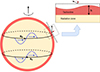 |
Fig. 1. Geometry of the problem; namely, the beta-plane approximation in which the equations are written in Cartesian coordinates in a plane tangent to the sphere at a given latitude, and the so-called beta-effect results from the meridional gradient of the local vertical component of the Coriolis parameter. A constant background magnetic field is considered at the reference latitude pointing in the x (east-west) direction, resulting in Rossby waves that will have both velocity and magnetic field perturbations that propagate in the x direction. |
 (1)
(1)
 (2)
(2)
 (3)
(3)
 (4)
(4)
where D/Dt ≡ ∂/∂t + u.∇, u = (u, v) is the horizontal velocity field and its zonal and meridional components, B = (Bx, By) is the horizontal magnetic field and its zonal and meridional components, h represents the thickness of the fluid layer, and f = 2Ωsin(θ) is the Coriolis parameter, with Ω representing the Sun’s rotation rate, and θ = θ(y) being the latitude. The ⊥ superscript denotes the perpendicular of a vector. Expressions of mid-latitude waves on Cartesian coordinates (beta-plane) can be found in several studies (Zaqarashvili et al. 2007; Teruya et al. 2022) and will be described below.
3.2. Magneto-inertio-gravity waves
The dispersion relation of the magneto-inertio-gravity waves was obtained by linearizing equations (4) upon a basic state that consists of a toroidal (zonal) magnetic field,  , and a fluid layer with average height H. First, we assume a resting basic velocity field of
  . The Coriolis parameter, f, is assumed to be constant, in the so-called f-plane approximation, f = f0 = 2Ωsin(θ0), around a reference latitude, θ0. Then, we assume a plane wave ansatz,
  , where
  is the wavenumber with its respective zonal and meridional components, and ω is the respective eigenfrequency with the respective eingenvector,
  . The resulting frequency is therefore
 (5)
(5)
where  is the pure gravity wave velocity (nonrotating) and
  is the Alfvén wave velocity. H represents the thickness of the fluid layer and g the effective gravity (Horstmann et al. 2023). We note that this dispersion relation is bounded from below by the frequency given by the Coriolis parameter at the origin.
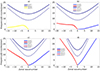 |
Fig. 2. Dispersion relation of fast (FM) and slow (SM) Rossby modes as well as inertio-gravity (IG) modes, respectively, using the f-plane and the beta-plane approximations at 30° (solid lines) and 15° (dotted lines) for several magnitudes of the toroidal tacholine magnetic field. It starts from panel (a) 0 kG, where the waves are purely hydrodynamic and there is only one Rossy mode, the hydrodynamic Rossby mode (HD). By increasing the intensity of the magnetic field to (b) 5 kG, (c) 15 kG, and (d) 30 kG, we notice that the dispersion relations become increasingly steep. |
3.3. Magneto-Rossby waves
Next, instead of using the f-plane approximation, where the Coriolis parameter is assumed to be constant in the meridional direction, we used the beta-plane approximation in which the Coriolis parameter is assumed to vary linearly with the meridional coordinate, y. This was done by setting f = f0 + βy, where β = 2Ωcos(θ0)/a, where a is the radius of the Sun at the tachocline and θ0 a reference latitude. The easiest way to obtain the dispersion relation of the magneto-Rossby waves is to derive a magnetohydrodynamic barotropic vorticity equation from the magneto-shallow water equations (Eq. (4)). This was done by taking ∂/∂y of the u component of Eq. (4) and subtracting it from ∂/∂x of the v component of Eq. (4). By doing so, we obtained the following system:
 (6a)
(6a)
 (6b)
(6b)
where ψ is the stream function (u, v)=(−∂ψ/∂y, ∂ψ/∂x), q = ∇2ψ + βy is the potencial vorticity, A is the magnetic potential, (bx, by)=(−∂A/∂y, ∂A/∂x), and j = ∇2A is the magnetic current. The Jacobian operator is given by
 (7)
(7)
for any differentiable functions, f and g. By assuming an ansatz of the form  , as before,
  is the wavenumber with its respective zonal and meridional components, and ωR is the magneto-Rossby wave eigenfrequency with the respective eingenvector,
  . The resulting dispersion relation is
 (8)
(8)
giving rise to two branches, depending on the ± sign in front of the square root: one westward branch ( − ) and one eastward branch ( + ). It should be noted that in the formulation followed here, in Eq. (6), there are no pressure effects, since the curl operator is applied to the momentum equations. As such, the magneto-Rossby waves presented here are affected by magnetic tension and the Coriolis force, and not by any kind of pressure. Consequently, magneto-Rossby waves are a hybrid between Alfvén and hydrodynamic Rossby waves. This contrasts with magneto-inertio-gravity waves, which are strongly affected by pressure, being a hybrid between hydrodynamic inertio-gravity waves and MHD waves, which are not necessarily Alfvén waves (in most cases, degenerate slow magneto-acoustic waves), and which can propagate in any direction, not only along the background magnetic field.
Here, we are interested in comparing the dispersion relations of shallow-water magnetohydrodynamic waves, as is described above, with bright-point observations that are provided on a Carrington rotation frame. As such, we need to represent the theoretically derived dispersion curves not in the local frame sitting in the local tachocline rotation, but in the Carrington frame. The dispersion curves described above (Eqs. (5) and (8)) were derived in the local tachocline frame using the tachocline differential rotation parameters obtained in Dikpati & Charbonneau (1999) as a function of latitude and depth. When changing it to the Carrington frame, a Doppler shift effect appears. If ωT is the dispersion relation of a given wave represented in the tachocline frame at latitude θ and radius r, then for an observer sitting on a Carrington rotating frame the frequency, ωC, will be transformed as (Teruya et al. 2022)
 (9)
(9)
where U(θ, r) represents the difference in the velocities of both frames at a given latitude and radius, and k a given wavenumber.
In Figs. 2 and 3, we provide the dispersion curves, in the Carrington frame for differential rotation parameters of the base and the middle of the tachocline, respectively. Their interpretation will be discussed in the results section.
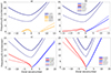 |
Fig. 3. Same as Fig. 2 but taking into account a Doppler shift correction because observations were performed in the Carrington frame of reference as well as tachocline differential rotation, with differential rotation parameters taken for the middle of the tachocline layer; namely, the rotation period at 30° latitude of 26.5 days, and a rotation period at 15° latitude of 26.1 days. (a) Dispersion relations (0kG). (b) Dispersion relations (5kG). (c) Dispersion relations (15kG). (d) Dispersion relations (30kG). |
4. Results
Two snapshots of the global distribution of BP density data are shown in Fig. 4 for two different dates separated by 20 days (February 21, 2012, and March 12, 2022). Two features are readily observed from these maps: (i) a degree of spatial organization and (ii) the persistence of large-scale patterns over several weeks. This suggests the existence of large-scale long-lived flow patterns that dictate the spatial distribution of BP. Previous studies (McIntosh et al. 2017, 2014, 2015; Dikpati & McIntosh 2020) have used BP datasets as a marker of large-scale coherent flows in the Sun, suggesting that their large-scale patterns are determined by Rossby waves. Similarly, cloud coverage data on Earth’s atmosphere has been used as a marker of wave activity, and employed in the calculations of wavenumber × frequency spectra clearly showing signatures of Rossby, Kelvin, Yanai, and inertio-gravity waves (Takayabu 1994; Wheeler & Kiladis 1999; Kiladis et al. 2009; Raphaldini et al. 2023a).
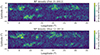 |
Fig. 4. BP density maps for two different days separated by 20 days. |
The main method was proposed by Wheeler & Kiladis (1999) and consists of computing Fourier transforms in longitude and time. A smoothing filter is then applied to the original spectrum. Finally, the raw spectrum is divided by the smoothed spectrum. This procedure will therefore produce a nondimensional spectrum highlighting local spectral maxima. Here, we demonstrate the application of the Wheeler-Kiladis procedure for two selected latitudes, 30° and 15°. For each selected latitude, θ, we computed the average BP density in a latitudinal strip (θ − 2° ,θ + 2° ) for all longitudes and all times. The results are described below.
4.1. Wavenumber × frequency spectral analysis
Figure 5 addresses the propagation of BP at ±30° latitude. The time × frequency diagram, also known as the Hovmöller Diagram (Figs. 5a, b), shows a predominantly retrograde propagation of the BP signal both in the northern (a) and southern (b) hemispheres. Comparing the northern and southern hemisphere diagrams, similar propagation speeds of ∼75 m/s are observed (at solar surface radii). Furthermore, it is noticeable that there is a stronger BP density signal in the first half of this period in the northern hemisphere, while the BP density signal becomes stronger in the southern hemisphere later. This is compatible with the pronounced north-south asymmetry of solar cycle 24 (Chowdhury et al. 2019). The wavenumber × frequency spectral analysis is presented in Fig. 5c, where we use the common convention in the meteorological literature, with negative wavenumbers indicating retrograde propagation. The resulting wavenumber × frequency spectrum shows a strong signal in the low frequency range (≤10 cycles/year), with a predominance of retrograde propagation, with some prograde propagation for low (k ≤ 5) wavenumbers. A second branch of strong BP density spectra signal is observed for higher wavenumbers in the range of 15−25 cycles per year.
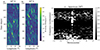 |
Fig. 5. Wave propagation properties at 30°. (a) and (b) represent, respectively, the Hovmoller (time × longitude) diagram at 30° latitudes in the northern and southern hemispheres. (c) represents the wavenumber × frequency spectrum at the same latitude. |
A similar analysis was performed by sampling the BP-density data at ±15° latitudes. The resulting Hovmöller diagram is shown in Fig. 6. This time, the propagation pattern in the BP density data reveals a slightly prograde propagation in both the northern and southern hemispheres with an average velocity of ∼+20 m/s, as is observed at the photospheric radii. The respective wavenumber × frequency spectrum is presented in Fig. 6c, where again there is a clear separation between slow (≤10 cycles/year) and fast (≥10 cycles/year) frequency oscillations. As was expected from the Hovmöller diagram, the predominance in the low frequency range is toward positive (eastward) propagation.
 |
Fig. 6. Wave propagation properties at 15°. (a) and (b) represent, respectively, the Hovmoller (time × longitude) diagram at 15° latitudes in the northern and southern hemispheres. (c) represents the wavenumber × frequency spectrum at the same latitude. |
4.2. Comparison with theoretical dispersion relations
One of the interesting properties of the magneto-Rossby waves is that, for large zonal wavenumbers, k, the respective dispersion relations, ωR(k), get closer and closer to the dispersion relations of the (dispersionless) Alfvén waves,  , where B0 is the magnetic field strength, μ0 the magnetic permeability of the vacuum, and ρ the density of the plasma. This property means that the larger B0 is the background magnetic field and k is the zonal component (parallel to the background magnetic field). The steeper the dispersion curves, the more magneto-Rossby waves will behave like Alfvén waves. This can be noted by the dispersion relation expression, which can be written in the following form:
 (10)
(10)
where vMR, vR, and vA are, respectively, the phase velocities of the magneto-Rossby, pure Rossby, and Alfvén waves, the last two given by
 (11)
(11)
Therefore, for large enough B0, we have that |vA|≫|vR|, and consequently vMR ≈ ±vA, keeping in mind that there are two magneto-Rossby modes.
Figure 2 displays the dispersion relation of magneto-Rossby and magneto-inertio-gravity waves for the selected latitudes (30° and 15°) and magnetic field strengths: (a) 0 kG, (b) 5 kG, (c) 15 kG, and (d) 30 kG. Starting at 0 kG, the two branches of magneto-Rossby waves degenerate to a single branch that represents the purely hydrodynamic Rossby waves for which the corresponding frequency decreases as |k| increases. In the presence of a magnetic field, there are two branches of magneto-Rossby waves, one with prograde propagation and one with retrograde propagation. For a weak magnetic field, the corresponding frequencies will slowly increase with |k|. By considering stronger magnetic fields of 15 kG (c) and 30 kG (d), frequencies become higher more rapidly. More details on the dispersion curves are presented in the methods section.
Magneto-inertio-gravity waves are also modified by the underlying magnetic field in such a way that the dispersion curves become steeper and steeper as the magnetic field strength increases. This is again illustrated in Fig. 2, where we notice that the respective frequencies change from slowly increasing with |k| in the nonmagnetic case (a). As the magnetic field strength is increased to 5 kG (b), 15 kG (c), and 30 kG (d), the dispersion curves become steeper and steeper. This dispersion relation was calculated at the radiative zone rotation frame (with a rotation period of TCR ≈ 26.74 days). In order to compare the dispersion curves with observations, one needs to account for the fact that the observer is at the Carrington frame. If we consider the differential rotation at the middle of the tachocline (Dikpati & Charbonneau 1999; Garaud & Guervilly 2009), we obtain a rotation period at 30° latitude of T30 ≈ 26.5 days, and a rotation period at 15° latitude of T15 ≈ 26.1 days, while one full revolution in the Carrington frame is TCR ≈ 27.28 days. This results in a Doppler shift, which makes the dispersion curves asymmetric.
We can compare the resulting dispersion curves presented in Fig. 3 with the wavenumber × frequency spectra presented in Figs. 5 and 6. An important feature that can be observed in both the wavenumber × frequency and the Hovmöller diagram is that from 30° to 15°, the propagation patterns of BPs change from predominantly negative to positive propagation, while theoretically derived dispersion relations modified by differential rotation change from negative to positive propagation for weaker magnetic fields, B ≲ 15 kG (see Fig. 3). Although this does not exclude the possibility of stronger magnetic fields confined to the tachocline, it suggests an upper limit for the magnetic field strength from where magnetic field emergence originates. This analysis therefore provides an important constraint on solar dynamo models (Guerrero et al. 2019).
5. Discussion
We have presented a wavenumber × frequency of global solar oscillations from coronal BPs. Inertial waves present at the tachocline layer, such as the magneto-Rossby waves and the magneto-inertio-gravity waves, are influenced by rotation, magnetic fields, and the stratification properties of this region. In particular, the strength of the tachocline magnetic field is poorly constrained, with estimates primarily based on numerical dynamo models, although it is agreed that the 100 kG value is probably an upper limit on the possible value (Strugarek et al. 2023). Although 100 kG magnetic fields, or ones even stronger than that, could be generated in the Sun, the question is what strength is actually contributing to what manifests at the surface in the form of various magnetic features. Both magneto-Rossby and magneto-inertio-gravity waves have the property that their dispersion relation becomes steeper for large zonal wavenumbers as the magnetic field strength increases. Therefore, from the derivation of this property of the tachocline waves, we suggest that, if the tachocline magnetic fields at or near the convection zone base are contributing to the production of the surface magnetic features, a strength of up to 15 kG should be sufficient.
It should be noted that this estimate is valid for the rising or peak phase of solar cycle 24, when the global reconstruction of BP density was possible due to the appropriate positions of the STEREO and SDO missions during the 2010−2013 period (McIntosh et al. 2017). Since solar cycle 24 was weak (Jiang et al. 2015), it is likely that a typical cycle would provide slightly larger estimates for the tachocline field strength. Our estimate is roughly compatible with the estimate obtained in Gurgenashvili et al. (2016) for weak cycles.
Recently, Korsós et al. (2023) analyzed short periodicities using magnetic field synoptic maps as well as the McIntosh archive, which includes numerous solar features. Dominant periods were found to exist at 185−195 days and 150−160 days. These periods were found in both latitudinal and longitudinal feature movements that can be associated with the tracer transport under the influence of Rossby waves, suggesting that these waves constitute a mechanism for the Rieger-type oscillations. This is compatible with the dominant low-frequency band of roughly 2 oscillations per year seen in Figs. 5 and 6. Korsós et al. (2023) also report differences in the dominant frequencies between cycles 23 and 24, according to the discussion presented here. This could be due to two main reasons: (1) differences in the strength of the toroidal fields in the tachocline that would impact the linear dispersion relation (8), or (2) nonlinear effects that would alter the oscillation frequencies for large enough wave amplitudes (Raphaldini et al. 2019).
Here, we have explored only linear effects on a single-layer model. In future work, we shall explore in a two-layer model how stratification effects modify the frequencies of Rossby and inertio-gravity waves; in particular, the behavior of “internal” modes (i.e., those in which perturbation fields vary with height), as well as modifications of the frequencies by nonlinear effects (Raphaldini et al. 2019, 2020; Dikpati et al. 2018). Synchronous datasets for periods approaching solar minima could provide evidence for equatorially trapped waves that were recently theorized to exist (Zaqarashvili 2018). This highlights the importance of continuous global (360°) observations of the Sun for unveiling properties of the Sun’s interior, and ultimately helping to predict space weather.
Acknowledgments
This work is supported by the National Center for Atmospheric Research, which is a major facility sponsored by the National Science Foundation under cooperative agreement 1852977. We acknowledge support from several NASA grants, namely, M.D. and B.R. acknowledge NASA-LWS grant No. 80NSSC20K0355 and NASA-HSR grant No. 80NSSC21K1676 and COFFIES Phase II NASA-DRIVE Center for the subaward from Stanford with grant No. 80NSSC22M0162. MD also acknowledges support through subaward from JHU/APL with NASA-HSR grant 80NSSC21K1678. A.S.W.T. has been supported by Fundação de Amparo à Pesquisa do Estado de São Paulo (FAPESP; grant 2020/14162-6).
References
- Berdyugina, S., & Usoskin, I. 2003, A&A, 405, 1121 [NASA ADS] [CrossRef] [EDP Sciences] [Google Scholar]
- Boers, N., Goswami, B., Rheinwalt, A., et al. 2019, Nature, 566, 373 [NASA ADS] [CrossRef] [Google Scholar]
- Brun, A. S., Miesch, M. S., & Toomre, J. 2004, ApJ, 614, 1073 [Google Scholar]
- Castenmiller, M., Zwaan, C., & Van der Zalm, E. 1986, Sol. Phys., 105, 237 [CrossRef] [Google Scholar]
- Chowdhury, P., Kilcik, A., Yurchyshyn, V., et al. 2019, Sol. Phys., 294, 1 [NASA ADS] [CrossRef] [Google Scholar]
- Dikpati, M., & Charbonneau, P. 1999, ApJ, 518, 508 [NASA ADS] [CrossRef] [Google Scholar]
- Dikpati, M., & McIntosh, S. W. 2020, Space Weather, 18, e2018SW002109 [NASA ADS] [CrossRef] [Google Scholar]
- Dikpati, M., Cally, P. S., McIntosh, S. W., et al. 2017, Sci. Rep., 7, 14750 [NASA ADS] [CrossRef] [Google Scholar]
- Dikpati, M., McIntosh, S. W., Bothun, G., et al. 2018, ApJ, 853, 144 [Google Scholar]
- Dikpati, M., McIntosh, S. W., Chatterjee, S., et al. 2021, ApJ, 910, 91 [NASA ADS] [CrossRef] [Google Scholar]
- Dikpati, M., Gilman, P. A., Guerrero, G. A., et al. 2022, ApJ, 931, 117 [NASA ADS] [CrossRef] [Google Scholar]
- Farrell, B. F., & Ioannou, P. J. 2009, J. Atmos. Sci., 66, 3197 [CrossRef] [Google Scholar]
- Garaud, P., & Guervilly, C. 2009, ApJ, 695, 799 [NASA ADS] [CrossRef] [Google Scholar]
- Gilman, P. A. 2000, ApJ, 544, L79 [NASA ADS] [CrossRef] [Google Scholar]
- Guerrero, G., Zaire, B., Smolarkiewicz, P., Dal Pino, E. D. G., et al. 2019, ApJ, 880, 6 [NASA ADS] [CrossRef] [Google Scholar]
- Gurgenashvili, E., Zaqarashvili, T. V., Kukhianidze, V., et al. 2016, ApJ, 826, 55 [NASA ADS] [CrossRef] [Google Scholar]
- Hanson, C. S., Hanasoge, S., & Sreenivasan, K. R. 2022, Nat. Astron., 6, 708 [NASA ADS] [CrossRef] [Google Scholar]
- Harris, J., Dikpati, M., Hewins, I. M., et al. 2022, ApJ, 931, 54 [CrossRef] [Google Scholar]
- Hindman, B. W., & Jain, R. 2022, ApJ, 932, 68 [NASA ADS] [CrossRef] [Google Scholar]
- Horstmann, G. M., Mamatsashvili, G., Giesecke, A., et al. 2023, ApJ, 944, 48 [NASA ADS] [CrossRef] [Google Scholar]
- Hoskins, B. J., & Ambrizzi, T. 1993, J. Atmos. Sci., 50, 1661 [NASA ADS] [CrossRef] [Google Scholar]
- Hughes, D. W., Rosner, R., & Weiss, N. O. 2007, The Solar Tachocline (Cambridge: Cambridge University Press) [CrossRef] [Google Scholar]
- Jiang, J., Cameron, R. H., & Schuessler, M. 2015, ApJ, 808, L28 [NASA ADS] [CrossRef] [Google Scholar]
- Kiladis, G. N., Wheeler, M. C., Haertel, P. T., et al. 2009, Rev. Geophys., 47, RG2003 [CrossRef] [Google Scholar]
- Korsós, M. B., Dikpati, M., Erdélyi, R., et al. 2023, ApJ, 944, 180 [CrossRef] [Google Scholar]
- Löptien, B., Gizon, L., Birch, A. C., et al. 2018, Nat. Astron., 2, 568 [Google Scholar]
- Majda, A. 2003, Introduction to PDEs and Waves for the Atmosphere and Ocean (American Mathematical Soc.) [Google Scholar]
- Mathis, S. 2009, A&A, 506, 811 [CrossRef] [EDP Sciences] [Google Scholar]
- McIntosh, S. W., & Gurman, J. B. 2005, Sol. Phys., 228, 285 [NASA ADS] [CrossRef] [Google Scholar]
- McIntosh, S. W., Davey, A. R., Hassler, D. M., et al. 2007, ApJ, 654, 650 [NASA ADS] [CrossRef] [Google Scholar]
- McIntosh, S. W., Wang, X., Leamon, R. J., et al. 2014, ApJ, 792, 12 [NASA ADS] [CrossRef] [Google Scholar]
- McIntosh, S. W., Leamon, R. J., Krista, L. D., et al. 2015, Nat. Commun., 6, 6491 [NASA ADS] [CrossRef] [Google Scholar]
- McIntosh, S. W., Cramer, W. J., Pichardo Marcano, M., et al. 2017, Nat. Astron., 1, 0086 [CrossRef] [Google Scholar]
- Raphaldini, B., Teruya, A. S., Raupp, C. F., et al. 2019, ApJ, 887, 1 [NASA ADS] [CrossRef] [Google Scholar]
- Raphaldini, B., Medeiros, E., Raupp, C. F., et al. 2020, ApJ, 890, L13 [NASA ADS] [CrossRef] [Google Scholar]
- Raphaldini, B., Dikpati, M., & McIntosh, S. W. 2023a, ApJ, 953, 156 [NASA ADS] [CrossRef] [Google Scholar]
- Raphaldini, B., Dikpati, M., Norton, A. A., et al. 2023b, ApJ, 958, 175 [NASA ADS] [CrossRef] [Google Scholar]
- Salmon, R. 1998, Lectures on Geophysical Fluid Dynamics (Oxford: Oxford University Press) [Google Scholar]
- Strugarek, A., Belucz, B., Brun, A. S., et al. 2023, Space Sci. Rev., 219, 87 [NASA ADS] [CrossRef] [Google Scholar]
- Takayabu, Y. N. 1994, J. Meteorol. Soc. Jpn. Ser. II, 72, 433 [CrossRef] [Google Scholar]
- Teruya, A. S., Raphaldini, B., & Raupp, C. F. 2022, Front. Astron. Space Sci., 9, 856912 [NASA ADS] [CrossRef] [Google Scholar]
- Teruya, A. S., Raphaldini, B., Mayta, V., et al. 2023, Atmosphere, 14, 622 [NASA ADS] [CrossRef] [Google Scholar]
- Triana, S. A., Guerrero, G., Barik, A., et al. 2022, ApJ, 934, L4 [NASA ADS] [CrossRef] [Google Scholar]
- Usoskin, I. G. 2017, Liv. Rev. Sol. Phys., 14, 3 [Google Scholar]
- Wheeler, M., & Kiladis, G. N. 1999, J. Atmos. Sci., 56, 374 [CrossRef] [Google Scholar]
- Zaqarashvili, T. 2018, ApJ, 856, 32 [NASA ADS] [CrossRef] [Google Scholar]
- Zaqarashvili, T., Oliver, R., Ballester, J., et al. 2007, A&A, 470, 815 [NASA ADS] [CrossRef] [EDP Sciences] [Google Scholar]
- Zaqarashvili, T. V., Carbonell, M., Oliver, R., et al. 2010a, ApJ, 709, 749 [NASA ADS] [CrossRef] [Google Scholar]
- Zaqarashvili, T. V., Carbonell, M., Oliver, R., et al. 2010b, ApJ, 724, L95 [NASA ADS] [CrossRef] [Google Scholar]
- Zaqarashvili, T. V., Oliver, R., Hanslmeier, A., et al. 2015, ApJ, 805, L14 [NASA ADS] [CrossRef] [Google Scholar]
- Zeitlin, V. 2013, Nonlinear Process. Geophys., 20, 893 [NASA ADS] [CrossRef] [Google Scholar]
All Figures
|
Fig. 1. Geometry of the problem; namely, the beta-plane approximation in which the equations are written in Cartesian coordinates in a plane tangent to the sphere at a given latitude, and the so-called beta-effect results from the meridional gradient of the local vertical component of the Coriolis parameter. A constant background magnetic field is considered at the reference latitude pointing in the x (east-west) direction, resulting in Rossby waves that will have both velocity and magnetic field perturbations that propagate in the x direction. |
| In the text | |
|
Fig. 2. Dispersion relation of fast (FM) and slow (SM) Rossby modes as well as inertio-gravity (IG) modes, respectively, using the f-plane and the beta-plane approximations at 30° (solid lines) and 15° (dotted lines) for several magnitudes of the toroidal tacholine magnetic field. It starts from panel (a) 0 kG, where the waves are purely hydrodynamic and there is only one Rossy mode, the hydrodynamic Rossby mode (HD). By increasing the intensity of the magnetic field to (b) 5 kG, (c) 15 kG, and (d) 30 kG, we notice that the dispersion relations become increasingly steep. |
| In the text | |
|
Fig. 3. Same as Fig. 2 but taking into account a Doppler shift correction because observations were performed in the Carrington frame of reference as well as tachocline differential rotation, with differential rotation parameters taken for the middle of the tachocline layer; namely, the rotation period at 30° latitude of 26.5 days, and a rotation period at 15° latitude of 26.1 days. (a) Dispersion relations (0kG). (b) Dispersion relations (5kG). (c) Dispersion relations (15kG). (d) Dispersion relations (30kG). |
| In the text | |
|
Fig. 4. BP density maps for two different days separated by 20 days. |
| In the text | |
|
Fig. 5. Wave propagation properties at 30°. (a) and (b) represent, respectively, the Hovmoller (time × longitude) diagram at 30° latitudes in the northern and southern hemispheres. (c) represents the wavenumber × frequency spectrum at the same latitude. |
| In the text | |
|
Fig. 6. Wave propagation properties at 15°. (a) and (b) represent, respectively, the Hovmoller (time × longitude) diagram at 15° latitudes in the northern and southern hemispheres. (c) represents the wavenumber × frequency spectrum at the same latitude. |
| In the text | |
Current usage metrics show cumulative count of Article Views (full-text article views including HTML views, PDF and ePub downloads, according to the available data) and Abstracts Views on Vision4Press platform.
Data correspond to usage on the plateform after 2015. The current usage metrics is available 48-96 hours after online publication and is updated daily on week days.
Initial download of the metrics may take a while.