| Issue |
A&A
Volume 671, March 2023
|
|
|---|---|---|
| Article Number | A91 | |
| Number of page(s) | 9 | |
| Section | Stellar structure and evolution | |
| DOI | https://doi.org/10.1051/0004-6361/202243985 | |
| Published online | 09 March 2023 | |
Rossby waves on stellar equatorial β planes: Uniformly rotating radiative stars
1
Georg-August-Universität, Institut für Astrophysik, Friedrich-Hund-Platz 1, 37077 Göttingen, Germany
e-mail: This email address is being protected from spambots. You need JavaScript enabled to view it.
2
Department of Astronomy and Astrophysics at Space Research Center, School of Natural Sciences and Medicine, Ilia State University, Kakutsa Cholokashvili Ave. 3/5, Tbilisi 0162, Georgia
3
Evgeni Kharadze Georgian National Observatory, Abastumani, Adigeni 0301, Georgia
4
Institut of Physics, IGAM, University of Graz, Universitätsplatz 5, 8010 Graz, Austria
Received:
9
May
2022
Accepted:
2
January
2023
Abstract
Context. Rossby waves arise due to the conservation of total vorticity in rotating fluids and may govern the large-scale dynamics of stellar interiors. Recent space missions have collected a lot of information about the light curves and activity of many stars, which triggered observations of Rossby waves in the stellar surface and interiors.
Aims. We aim to study the theoretical properties of Rossby waves in stratified interiors of uniformly rotating radiative stars with a sub-adiabatic vertical temperature gradient.
Methods. We used the equatorial β plane approximation and linear vertical gradient of temperature to study the linear dynamics of equatorially trapped Rossby and inertia-gravity waves in interiors of radiative stars. The governing equation was solved by the method of separation of variables in the vertical and latitudinal directions.
Results. Vertical and latitudinal solutions of the waves are found to be governed by Bessel functions and Hermite polynomials, respectively. Appropriate boundary conditions at the stellar surface and poles define analytical dispersion relations for Rossby, Rossby-gravity, and inertia-gravity waves. The waves are confined in surface layers of 30–50 H0, where H0 is the surface density scale height, and they are trapped between the latitudes of ±600. Observable frequencies (normalised by the angular frequency of the stellar rotation) of Rossby waves with m = 1 (m = 2), where m is the toroidal wavenumber, are in the interval of 0.65–1 (1.4–2), depending on the stellar rotation, radius, and surface temperature.
Conclusions. Rossby-type waves can be systematically observed using light curves of Kepler and TESS (Transiting Exoplanet Survey Satellite) stars. Observations and theory then can be used for the sounding of stellar interiors.
Key words: stars: interiors / stars: oscillations / stars: rotation
© The Authors 2023
 Open Access article, published by EDP Sciences, under the terms of the Creative Commons Attribution License (https://creativecommons.org/licenses/by/4.0), which permits unrestricted use, distribution, and reproduction in any medium, provided the original work is properly cited.
This article is published in open access under the Subscribe to Open model. This email address is being protected from spambots. You need JavaScript enabled to view it. to support open access publication.
1. Introduction
Rossby (planetary) waves are essential features of large-scale dynamics of rotating fluids. The theoretical background for the waves was first explored by Hadley (1735,), while Laplace tidal equations created the basics for the mathematical description (Laplace 1893). Hough (1897, 1898) found the solutions of the Laplace equations for the Rossby waves (low frequency solution in Hough’s terminology). However, the physical meaning of the waves was first described by Rossby (1939): the waves arise due to the conservation of total vorticity (planetary+relative) on a rotating sphere, which drives the propagating oscillations in the opposite direction of rotation.
Rossby waves are well studied in the Earth’s context by observations and theory. Westward propagating waves with a predicted phase speed have been continuously observed in the terrestrial atmosphere (Hovermoller 1949; Eliasen & Machenhauer 1965; Yanai & Lu 1983; Lindzen et al. 1984; Hiroota & Hirota 1989; Madden 2007) and oceans (Chelton & Schlax 1996; Hill et al. 2000). The theory of terrestrial Rossby waves is also well studied (Haurwitz 1940; Lindzen 1967; Gill 1982; Pedlosky 1987). The detailed dynamics of the Rossby waves in the Earth’s atmosphere and oceans is summarised in the reviews of Platzman (1968) and Salby (1984).
Recent direct observations of Rossby waves in the solar surface (Löpten et al. 2018) revived the interest for the study of Rossby waves on the Sun. The waves were observed by different methodologies such as granular tracking and helioseismology (Liang et al. 2019; Hanasoge & Mandal 2019; Proxauf et al. 2020; Gizon et al. 2021; Hanson et al. 2022). The Rossby wave signature was also found in the dynamics of solar coronal bright points (McIntosh et al. 2017; Krista & Reinard 2017). It was suggested that the magnetic Rossby waves may influence the short-term activity variations in the solar dynamo layer below the convection zone (Zaqarashvili et al. 2010; Zaqarashvili 2018; Dikpati et al. 2018, 2020). The Rossby waves are important in the dynamics of many astrophysical objects such as Solar System planets, exoplanets, accretion disks, among others (Zaqarashvili et al. 2021).
The recent space missions CoRoT (Convection, Rotation and planetary Transits), Kepler, and TESS (Transiting Exoplanet Survey Satellite) have collected a lot of information about stellar light curves and activity. Van Reeth et al. (2016) reported the detection of Rossby waves in rapidly rotating γ Dor stars in period spacing patterns. The pressure field of Rossby waves on the stellar surface may influence their light curves as suggested by Saio et al. (2018), hence the waves have been continuously observed in many Kepler stars with different spectral types (Saio et al. 2018; Li et al. 2019; Jeffery 2020; Samadi-Ghadim et al. 2020; Takata et al. 2020; Henneco et al. 2021; Saio & Kurtz 2022). Lanza et al. (2019) show that the Rossby waves may represent a source of confusion in the case of slowly rotating inactive stars that are preferential targets for a radial velocity planet search. Therefore, the theoretical description of stellar Rossby waves is important for stellar activity and exoplanetary research.
Rossby waves have been known as r modes in the stellar community since Papaloizou & Pringle (1978). Provost et al. (1981) made significant progress in the theoretical study of r modes in uniformly rotating stars by perturbation analysis (see also Damiani et al. 2020 for a similar topic of study). Saio (1982) examined the r-mode oscillations in the massive zero-age main sequence and ZZ Ceti stars. The studies generally concerned the slowly rotating stars, which allowed for perturbation analysis by a small expansion parameter for slow rotation (we note that Papaloizou & Pringle 1978 studied rapidly rotating stars, but for the high order harmonics of r modes). On the other hand, it is of vital importance to study the Rossby waves for stars with any rotation rate.
Here we aim to study the Rossby waves in stratified stellar interiors without approximation of slow rotation. We use the formalism of terrestrial Rossby waves, which has been well tested in Earth’s atmosphere (e.g., Lindzen 1967). The formalism allowed us to derive the exact solutions and dispersion relations for Rossby, Rossby-gravity, and inertia-gravity waves in rectangular equatorial β plane approximation. The periods of different harmonics can be used for observations of the waves in stellar light curves. In this paper, we are concerned with the radiative stars without an outer convection zone.
2. Governing equations
We started with linearised momentum, continuity, and energy equations in a frame of a uniformly rotating star:
 (1)
(1)
 (2)
(2)
 (3)
(3)
where v is the velocity, ρ0 (p0) is the unperturbed density (pressure), p′ (ρ′) is the perturbation of pressure (density), g is the gravitational acceleration, Ω is the angular velocity of rotation, and γ = cp/cv is the ratio of specific heats.
In the following, we adopt the Cartesian coordinates (x, y, z), where x is directed towards rotation, y is directed towards the north pole, and z is directed vertically upwards. An undisturbed medium was assumed to be in vertical hydrostatic balance
 (4)
(4)
and the ideal gas law is written as
 (5)
(5)
where kb is the Boltzman constant, T(z) is the temperature, m is the mass of hydrogen atom, and H(z) = kbT(z)/mg is the density scale height. Then the substitution of Eq. (5) into Eq. (4) gives the vertical distribution of the density governed by the equation
 (6)
(6)
We closely followed to the formalism of Lindzen (1967), who considered the β plane approximation for the uniform temperature with depth. Our calculation, however, was performed for a non-uniform distribution of temperature with depth. Here we use the vertically hydrostatic assumption, which means that the vertical distribution of the pressure is only slightly disturbed from its static form as it is typical for geophysical and astrophysical flows with a small Rossby number. This means that the vertical velocity is small and it is neglected in the vertical momentum equation, while it is kept in the continuity equation. This approximation does not take internal gravity or acoustic waves into account and hence it is only valid for long-period waves.
We changed variables as
 (7)
(7)
so that Eqs. (1)–(3) could be written after the Fourier transform with ei(−σt + kx) as
 (8)
(8)
 (9)
(9)
 (10)
(10)
 (11)
(11)
![Mathematical equation: $$ \begin{aligned}&i \sigma p^\prime = i\gamma g H \sigma \rho^\prime - g\left[1-\gamma \left(1+\frac{\mathrm{d} H}{\mathrm{d}z} \right)\right]{ v}_z, \end{aligned} $$](/articles/aa/full_html/2023/03/aa43985-22/aa43985-22-eq12.gif) (12)
(12)
where f = 2Ω sin θ is the Coriolis parameter with θ being a latitude (we note that the tilde sign was not used for the variables). Due to the vertically hydrostatic assumption, the two terms −iσvz and −2Ωyvx were omitted on the left-hand side of Eq. (10). The ratios of the omitted terms and the first term on the right-hand side of Eq. (10) are proportional to σ2H/g and RH/λ2, respectively, where R is the radius of the sphere and λ is the horizontal wavelength. The first ratio is very small for the Rossby wave timescales. The second ratio is proportional to H/R ≪ 1 for the typical Rossby wavelengths. Hence, both terms are small and a vertically hydrostatic assumption is justified in the current consideration of Rossby-type waves.
Equations (8) and (9) lead to the equation
 (13)
(13)
Eliminating ρ′, vz, and vx from Eqs. (10)–(12), we obtain
![Mathematical equation: $$ \begin{aligned}&\frac{\partial }{\partial z} \left[ \frac{\gamma H}{1-\gamma (1+H^{\prime })} \frac{\partial p^\prime }{\partial z} \right] \nonumber \\&-\left[ \frac{g k^2}{\sigma ^2} + \frac{\gamma (1+H^{\prime })^2}{4H[1-\gamma (1+H^{\prime })]} - \frac{\gamma H^{\prime \prime }}{2[1-\gamma (1+H^{\prime })]^2} \right] p^\prime \nonumber \\ &+ \frac{i g}{\sigma }\left[\frac{\partial }{\partial { y}} - \frac{k}{\sigma } f\right] { v}_{ y} = 0, \end{aligned} $$](/articles/aa/full_html/2023/03/aa43985-22/aa43985-22-eq14.gif) (14)
(14)
where H′ means the derivative of H by z.
We eliminated p′ from Eqs. (13)–(14) and derived the single equation for vy:
![Mathematical equation: $$ \begin{aligned}&\frac{\partial }{\partial z} \left[ \frac{\gamma H}{1-\gamma (1+H^{\prime })} \frac{\partial { v}_{ y}}{\partial z} \right] \nonumber \\&-\left[\frac{\gamma (1+H^{\prime })^2}{4H[1-\gamma (1+H^{\prime })]} - \frac{\gamma H^{\prime \prime }}{2[1-\gamma (1+H^{\prime })]^2} \right]{ v}_{ y}\nonumber \\&- \frac{g}{f^2 - \sigma ^2} \left(\frac{\partial ^2}{\partial { y}^2} - k^2 - \frac{k}{\sigma } \frac{\mathrm{d} f}{\mathrm{d}{ y}}\right) { v}_{ y} = 0. \end{aligned} $$](/articles/aa/full_html/2023/03/aa43985-22/aa43985-22-eq15.gif) (15)
(15)
This equation can be solved by the separation of variables in appropriate boundary conditions. Here we note that the separation of variables is only possible in the case of a vertically hydrostatic assumption.
We represent vy as
 (16)
(16)
and after straightforward calculations with the separation constant −h−1 we derived the two equations
![Mathematical equation: $$ \begin{aligned}&\frac{\partial ^2 \Psi }{\partial { y}^2} + \left[\frac{\sigma ^2 -f^2}{g h} - k^2 - \frac{k}{\sigma }\frac{\mathrm{d} f}{\mathrm{d}{ y}} \right] \Psi = 0, \end{aligned} $$](/articles/aa/full_html/2023/03/aa43985-22/aa43985-22-eq17.gif) (17)
(17)
![Mathematical equation: $$ \begin{aligned}&\frac{\partial }{\partial z} \left[ \frac{\gamma H}{1-\gamma (1+H^{\prime })} \frac{\partial }{\partial z} \right]V(z)\nonumber \\&-\left[ \frac{\gamma (1+H^{\prime })^2}{4H[1-\gamma (1+H^{\prime })]} - \frac{\gamma H^{\prime \prime }}{2[1-\gamma (1+H^{\prime })]^2} + \frac{1}{h} \right]V(z) = 0. \end{aligned} $$](/articles/aa/full_html/2023/03/aa43985-22/aa43985-22-eq18.gif) (18)
(18)
Here Eqs. (17) and (18) are the latitudinal and vertical equations governing the latitudinal and vertical structures of the waves, respectively. In fact, Eq. (17) is equivalent to the equation that governs shallow water equatorially trapped waves in a homogeneous layer with the width of h (e.g., Matsuno 1966). This conclusion corresponds to the Taylor theorem (Taylor 1936), which states that the dynamics of Rossby waves in stratified fluids is identical to the waves in a homogeneous layer that has a width of equivalent depth. The equivalent depth is different for different modes of Rossby waves. The theorem is valid for all compressible and stratified fluids (Pedlosky 1987; Zaqarashvili et al. 2021). We first solved Eq. (18) in appropriate surface boundary conditions and found the equivalent depth, h. Then we used it to solve Eq. (17) and found the solutions in the y direction, satisfying bounded boundary conditions at poles. It should be noted that the value of equivalent depth, h, found from Eq. (18) defines the solutions of Eq. (17); therefore, the two equations are not independent, but interconnected by h.
Before starting to study the case of inhomogeneous distribution of temperature with depth, we present the solutions of the simplest case of uniform H, which means an isothermal temperature profile. This is a very simplified approach, but it gives the basic physics of oscillations.
With H = const, Eq. (18) leads to
![Mathematical equation: $$ \begin{aligned} \frac{\partial ^2 V(z)}{\partial z^2}-\left[\frac{1}{4H^2}- \frac{\kappa }{ H h}\right] V(z) = 0, \end{aligned} $$](/articles/aa/full_html/2023/03/aa43985-22/aa43985-22-eq19.gif) (19)
(19)
where κ = (γ − 1)/γ.
The solution of Eq. (19) involves either exponential or periodic functions depending on the value of the equivalent depth, h. We considered the exponential function for the close boundary condition vz = 0 at the surface, which corresponds to z = 0. The value for the scale height depends on the surface temperature. The surface temperature of 10 000 K gives H = 300 km and the corresponding equivalent depth found from the close boundary condition is h ≈ 500 km.
The equivalent depth can be used to solve the latitudinal equation, Eq. (17). The solutions of Eq. (17) must satisfy boundary conditions in y directions, namely they must exponentially vanish at poles. Only the equivalent depth that satisfies the polar boundary conditions can be considered to be valid. The solution of the latitudinal equation for h = 500 km does not satisfy boundary conditions at poles; therefore, the exponential solution of Eq. (19) is not valid. The periodic solution of Eq. (19) leads to the value of equivalent depth, which satisfies the polar boundary conditions, but it corresponds to very high vertical wavenumber values.
When the temperature is a function of depth (generally increasing), then its gradient governs the state of the medium, which could be adiabatic, radiative, or convective. The Ledoux function, A, which defines the state, can be written using Eqs. (4)–(6) in terms of the density scale height as
 (20)
(20)
When |dH/dz|=|H′| > (γ − 1)/γ, that is A > 0, the temperature gradient is super-adiabatic and corresponds to convective stars. When |H′| < (γ − 1)/γ, in other words A < 0, the temperature gradient is sub-adiabatic, hence it corresponds to radiative stars. When A = 0, that is to say |H′| = κ = (γ − 1)/γ = 2/5, the star is neutrally stable so that the temperature gradient is adiabatic, which is a limiting case of super- and sub-adiabatic gradients. In this paper, we consider radiative stars; therefore, the condition of |H′| < κ should be satisfied everywhere. This condition is most easily satisfied for the linear profile of temperature with a uniform vertical gradient. For other profiles, the vertical temperature gradient generally increases with depth, which unavoidably leads to the violation of the radiative condition at some distance from the surface. Therefore, we assumed that the density scale height is a linear function of depth (readers should remember that z > 0 above the surface and z < 0 below the surface), that is
 (21)
(21)
This is equivalent to the temperature profile of the form
 (22)
(22)
where T0 is the temperature at the surface, z = 0. In this case, the radiative stars imply ϵ < κ and we use this criterion throughout the paper.
3. Free oscillations of radiative stars
We started to study free oscillations, meaning that we first solved the vertical structure Eq. (18) in corresponding boundary conditions. The solutions of the equation govern the spatial structure of Rossby waves along the vertical direction. The boundary conditions allowed us to find the discrete values of equivalent depth h. Then we used h to find latitudinal solutions of Eq. (17), which exponentially tend to zero at poles. These solutions correspond to the latitudinal structure of Rossby waves.
3.1. Vertical structure of Rossby waves
For the linear temperature profile, Eq. (18) is rewritten as
![Mathematical equation: $$ \begin{aligned} \frac{\partial }{\partial z} \left[ \frac{\gamma H}{1-\gamma (1+H^\prime )} \frac{\partial }{\partial z} \right] V(z)-\left[ \frac{\gamma (1+H^\prime )^2}{4H [1-\gamma (1+H^\prime )]} + \frac{1}{h} \right] V(z) = 0, \end{aligned} $$](/articles/aa/full_html/2023/03/aa43985-22/aa43985-22-eq23.gif) (23)
(23)
where H′=dH/dz. Using the new variable
 (24)
(24)
Eq. (23) leads to
 (25)
(25)
where n = (1 − ϵ)/ϵ. This is the Bessel equation and its solutions are Bessel functions of order n, Jn(x), and Yn(x). The solutions Jn(x) and Yn(x) must satisfy certain boundary conditions at the surface. We used two different boundary conditions. The first condition yields the vertical velocity vanishing at the surface, that is vz = 0 at z = 0, which is a close condition. The second condition yields the total Lagrangian pressure being zero at the surface, which is a free boundary condition. In both cases, vertical velocity and total pressure must be bounded towards the stellar centre.
We used different values of ϵ to find the vertical structure of Rossby waves for different vertical temperature gradients. We assumed ϵ = 0.2, 1/3, 0.39, which give the order of Bessel functions as n = 4, 2, 1.56, respectively. We note that the adiabatic temperature gradient corresponds to ϵ = 0.4, and therefore ϵ = 0.39 is nearly the upper limit of the radiative temperature gradient.
3.1.1. Close boundary condition, vz = 0, at the surface
The close boundary condition, vz = 0, from Eqs. (10)–(13) yields the following equation:
![Mathematical equation: $$ \begin{aligned} \frac{\partial { v}_{ y}}{\partial z} + \left[ \frac{1}{\gamma H} - \frac{1}{2H} - \frac{H^\prime }{2H} \right] { v}_{ y}=0. \end{aligned} $$](/articles/aa/full_html/2023/03/aa43985-22/aa43985-22-eq26.gif) (26)
(26)
Both solutions of Eq. (25), Jn(x) and Yn(x), have similar vertical structures to the modes. Therefore, we considered Jn(x) to be a solution and then Eq. (26) was rewritten as
![Mathematical equation: $$ \begin{aligned} \frac{\partial }{\partial x} J_n(x) + \frac{1}{x} \left[ \frac{1}{\epsilon } - 1 - \frac{2}{\gamma \epsilon } \right] J_n(x) = 0. \end{aligned} $$](/articles/aa/full_html/2023/03/aa43985-22/aa43985-22-eq27.gif) (27)
(27)
This is a transcendental equation, which has the infinite number of zeros. Each zero defines a certain value of equivalent depth, h, hence it corresponds to a certain wave mode. We first solved the equation for ϵ = 1/3 and, for the first six zeros, we obtained the values of equivalent depth as h ≈ 1.05 H0, h ≈ 0.058 H0, h ≈ 0.025 H0, h ≈ 0.014 H0, h ≈ 0.009 H0, and h ≈ 0.0064 H0, respectively. As we mentioned above, only the values of equivalent depth (or wave modes), which result in the bounded conditions at poles, are valid. Solutions of the latitudinal equation (see the next subsection) show that the modes corresponding to the first five zeroes do not satisfy polar boundary conditions and hence they are not valid. On the other hand, the modes corresponding to the sixth (and larger) zero satisfy bounded conditions at poles. The solutions of Eq. (27) for the temperature gradient of ϵ = 0.39 show that the mode, which corresponds to the second zero of the equation, already satisfies the polar boundary conditions. Therefore, all modes starting from the second mode in the vertical direction are valid for a nearly adiabatic temperature gradient. On the other hand, the temperature gradient of ϵ = 0.2 yields the 17th and higher modes giving the bounded polar boundary conditions. Figure 1 shows the vertical structure of Rossby waves based on the solutions of Eq. (25) for different values of ϵ. We see that all solutions exponentially decrease with depth, hence the corresponding modes are trapped near the surface. All higher modes show a similar behaviour. The figure shows that the smaller values of ϵ, that is the smaller temperature gradient, yield the shorter vertical wavelength of Rossby waves and the stronger decay of the wave amplitude with depth. Therefore, the Rossby waves tend to be concentrated closer to the surface for a smaller temperature gradient.
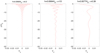 |
Fig. 1. Vertical structure of Rossby waves for different vertical temperature gradients: ϵ = 0.2 (left panel), ϵ = 1/3 (middle panel), and ϵ = 0.39 (right panel). Here vy is plotted without |

3.1.2. Free boundary condition
In the free surface condition, the total Lagrangian pressure is zero at the surface. Using Eqs. (10) and (12), the condition is
 (28)
(28)
which can be rewritten for the new variable x as
 (29)
(29)
This is also a transcendental equation and has an infinite number of zeros. We assumed ϵ = 1/3 and for the first five zeroes we found h ≈ 0.069 H0, h ≈ 0.027 H0, h ≈ 0.015 H0, h ≈ 0.0094 H0, and h ≈ 0.0065 H0, respectively. Only the modes corresponding to the fifth (and higher) zero satisfy the polar boundary conditions.
The value of h obtained from each zero with a free condition is similar to the value obtained from the next higher zero with a close condition. For example, the first zero with a free condition is near to the second zero with a close condition, etc. This happens because of the relation between the total Lagrangian pressure and vertical velocity. Therefore, close and free boundary conditions result in a similar spatial structure with a depth of the corresponding modes. Consequently, we only consider the closed boundary condition in the rest of the paper.
3.2. Latitudinal structure of Rossby waves
We now turn to the latitudinal equation (Eq. (17)) and find the solutions with certain h satisfying bounded conditions at poles, which define dispersion relations of possible wave modes in the system. The solutions of Eq. (17) crucially depend on the parameter
 (30)
(30)
which actually corresponds to the parameter (sometimes referred to as the Lamb parameter) governing the dynamics of shallow water system of the layer thickness h. When this parameter is much larger than one (for fast rotation or small h), then Eq. (17) is most easily satisfied for small y1. Small y is equivalent to the equatorial region and hence the solutions are equatorially trapped. Third and higher zeroes with a close boundary condition with h < 0.025 H0 lead to the Lamb parameter of ε > 10 for solar radius, surface temperature, and rotation. Therefore, the modes corresponding to the higher zeroes with a close boundary condition are confined near the equatorial regions and decay sufficiently fast towards the poles. The modes, hence, can be considered by the equatorial β plane approximation, which would mean expanding the Coriolis parameter near the equator θ ≈ 0 and retaining only the first order term, f = βy, where β = (2Ω/R). In this case Eq. (17) tends to
![Mathematical equation: $$ \begin{aligned} \frac{\partial ^2 \Psi }{\partial { y}^2} + \left[-\frac{k \beta }{\sigma } - k^2 + \frac{\sigma ^2}{c^2} - \frac{\beta ^2 { y}^2}{c^2} \right] \Psi = 0, \end{aligned} $$](/articles/aa/full_html/2023/03/aa43985-22/aa43985-22-eq32.gif) (31)
(31)
where  is the surface gravity speed for corresponding equivalent depth h, which was obtained from the vertical structure equation as shown in the previous subsections.
It must be noted that the solutions under equatorial β plane approximation fairly correspond to the solutions of the spherical case. In fact, the governing equation of equatorially trapped Rossby waves in β plane approximation is identical to the spherical case (Longuet-Higgins 1968; Zaqarashvili et al. 2021). Here we consider only the equatorially trapped waves for which the β plane approximation is justified.
Equation (31) is a parabolic cylinder equation which has bounded solutions when
 (32)
(32)
where l = 0, 1, 2, 3… Then the solution to this equation is
![Mathematical equation: $$ \begin{aligned} \Psi =\Psi _0 exp\left[-\frac{\beta }{2c}{ y}^2 \right] H_l \left(\sqrt{\frac{\beta }{c}}{ y} \right) ,\end{aligned} $$](/articles/aa/full_html/2023/03/aa43985-22/aa43985-22-eq35.gif) (33)
(33)
where Ψ0 is the value of vy at the equator, y = 0, and Hl is the Hermite polynomial of the order l. The solution is oscillatory inside the interval  and exponentially decreases towards poles outside. Smaller h or larger ε yields a stronger decrease in the solution. As it was discussed above, the values of h corresponding to the lower zeroes of Eqs. (27) and (29) lead to solutions which are not bounded at poles. The bounded solutions in the case of ϵ = 1/3, which are shown in Fig. 2, start to appear for the sixth (fifth) zero with a close (free) boundary condition, which yields h ≈ 0.0064 H0. In this case, the Lamb parameter is around ε ≈ 43 for the solar radius, surface temperature, and rotation. The temperature gradient of ϵ = 0.39 allows for the second (and higher) zero with a close vertical boundary condition to lead to the bounded solution along latitudes. The critical latitude was estimated as
  , which for l = 1 modes gives around ±400, that is the solutions are oscillatory in the latitudes of < 400 and exponentially decay for > 400. Therefore, the solutions are mostly concentrated between the latitudes ±600 and are negligible at poles satisfying the boundary conditions there.
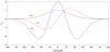 |
Fig. 2. Latitudinal structure of equatorially trapped Rossby waves for the temperature gradient of ϵ = 1/3 and the value of equivalent depth ≈0.0064 H0. The solutions exponentially decay towards poles above middle latitudes. Black, red, and blue curves show l = 0, l = 1, and l = 2 modes, respectively. |
3.3. Dispersion equation
Equation (32) defines the dispersion relation of waves
 (34)
(34)
This equation is identical to the dispersion relation of shallow water waves when the width of the shallow layer is replaced by the equivalent depth, h, as stated by the Taylor theorem. The dispersion relation governs the inertia-gravity, Rossby, and Rossby-gravity waves for each h.
For the high frequency limit (σ ≫ Ω) with l ≥ 1, we have the dispersion relation
 (35)
(35)
which corresponds to the inertia-gravity waves.
For the low frequency limit (σ ≪ Ω) with l ≥ 1, we have the dispersion relation
 (36)
(36)
which corresponds to the Rossby waves.
For l = 0, Eq. (34) leads to
 (37)
(37)
The first solution of Eq. (36) is spurious; therefore, it must be neglected and the second solution defines the Rossby-gravity wave
 (38)
(38)
The solutions of full dispersion equation (Eq. (34)) are displayed in Fig. 3 for ε = 43, which corresponds to the equivalent depth, h ≈ 0.0064 H0 (associated with the first valid vertical mode or the sixth zero with a close condition for the temperature gradient of ϵ = 1/3) and a star with the rotation, radius, and surface gravity of the Sun. We see that for large negative k, the dispersion curves of Rossby and Rossby-gravity waves merge, while for the large positive k the inertia-gravity and Rossby-gravity waves have the same behaviour. In the next subsection, we consider Rossby and Rossby-gravity waves in detail.
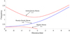 |
Fig. 3. Solutions of the full dispersion equation (Eq. (34)) for ε = 43, which corresponds to the first valid vertical mode (with h = 0.0064H0) in a star with the rotation, radius, and surface gravity of the Sun and the temperature gradient of ϵ = 1/3. Red curves correspond to the inertia-gravity (upper) and Rossby (lower) waves with l = 1. The blue curve corresponds to the Rossby-gravity waves with l = 0. Wave frequency was normalised by the angular frequency of the star, Ω. The toroidal wavenumber, k, was normalised by the stellar radius, R. |
3.4. Rossby and Rossby-gravity waves
Equation (36) is the dispersion relation for the Rossby waves on the equatorial β plane. The positive frequency and the negative toroidal wavenumber indicate the retrograde (opposite to the rotation) propagation of waves. The dispersion relation crucially depends on the parameter ε. When this parameter is small (that is for slowly rotating stars or large equivalent depth, h), then the second term in denominator is smaller than the first one, which eventually leads to the dispersion relation of Rossby waves on the 2D surface with only longitudinal propagation (ky = 0). This corresponds to sectoral harmonics in the spherical geometry. But a moderate value of the parameter significantly changes the dispersion relation of Rossby waves. In the considered case, this parameter has a moderate value due to the small h. For a star with solar parameters, that is T0 = 5770 K, Ω = 3 × 10⁻⁶ s−1, R = 7 × 10⁵ km, and h = 0.0064 H0 km as estimated in the previous subsection, one can find that ε ≈ 43. Therefore, one must keep the associated term in the dispersion relation. One should note that the parameter ε is equivalent to the parameter used by Provost et al. (1981) to study the r modes in slowly rotating stars, namely Ω2R3/(GM), if one replaces h by R and divides by four. Provost et al. (1981) expanded all variables and the frequency with this parameter assuming it to be much smaller than unity. This could be correct if the equivalent depth, h, is of the order of the stellar radius. But our solution shows that h ≪ R, that is the expansion parameter of Provost et al. (1981) is not small and cannot be appropriate in our consideration.
Rossby-gravity waves (l = 0) defined by Eq. (38) have mixed properties of Rossby and inertia-gravity waves. This mode is similar to Rossby waves when it propagates opposite to the rotation, but it is similar to the gravity wave when it propagates to the direction of the rotation. The wave has no oscillatory solution along latitudes and hence it corresponds to the sectoral modes in the spherical geometry.
4. Observational constraints
It is of importance to show how the theoretically obtained waves might be seen by observations. Recent progress in observations of Rossby waves using Kepler light curves suggest that the waves can also be detected in the data of the TESS mission. Here we provide hints for observers to detect the waves.
We used the rotating frame for the theoretical analysis of Rossby waves. On the other hand, observed light curves were obtained in the inertial frame; therefore, the observable frequency of the waves is expressed by
 (39)
(39)
where σ is the theoretical wave frequency in the rotating frame and m = kR is the normalised toroidal wavenumber.
Wave frequency depends on the parameter ε, which can be rewritten as
 (40)
(40)
where T0 (Tsun), Ω (Ωsun), and R (Rsun) are the surface temperature, the surface angular velocity, and the radius of a star (the Sun), respectively.
Figure 4 shows the dependence of the wave frequency in the inertial frame, σobs on ε. Only the frequency of lower order modes m = 1 and m = 2 are shown on this figure. The normalised frequencies of all modes (Rossby, Rossby-gravity, inertia-gravity) are increasing for higher ε, that is for the higher angular velocity of stars (with the same surface temperature and radius). The anti-symmetric harmonics with regards to the equator, l = 1, 3…, probably have negligible contributions to stellar light curves as the northern and southern parts of the modes cancel each other out2. Therefore, only symmetric harmonics, l = 0, 2, 4, are shown on this figure. Rossby waves with m = 1 have a frequency in the range of 0.65 Ω < σobs < Ω, that is less than the stellar angular velocity. The frequency of Rossby waves with m = 2 is in the range of 1.4 Ω < σobs < 2Ω. Inertia-gravity and Rossby-gravity waves have an order of magnitude higher frequencies than the angular velocity of stellar rotation. Observations can define the frequency of observed waves, which subsequently determine the corresponding value of ε using Fig. 4. It is important to note that ε depends on the equivalent depth, h, and three stellar parameters such as the surface temperature, the surface angular velocity, and the radius. The equivalent depth is calculated from the Rossby wave theory as discussed in the Sect. 3.1. Consequently, if one knows two of the stellar parameters, one can estimate the value of the third one.
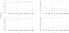 |
Fig. 4. Wave frequency in the inertial frame as expected to be seen by observations vs. ε. The frequency was normalised by the angular frequency of a star, Ω. Black, blue, and red curves correspond to the modes with l = 0, l = 2, and l = 4, respectively. The left panels display the Rossby modes with m = 1 (solid lines, upper panel) and m = 2 (dashed lines, lower panel). The upper (lower) right panel shows inertia-Gravity modes (Rossby-gravity modes). Grey dashed lines denote the value of ε calculated for the solar parameters and the equivalent depth of h = 0.0064 H0. |
5. Discussion and conclusions
Rossby waves arise due to the conservation of absolute vorticity; therefore, vorticity is an essential ingredient of the waves. On the other hand, pressure variation is an equally important component in the waves. Therefore, the waves cause the periodic variations of surface pressure (temperature or density or both), which may lead to the periodical modulation of stellar radiance (Saio et al. 2018). Recent observations of Rossby waves in the light curves of Kepler and TESS stars (Saio et al. 2018; Li et al. 2019; Jeffery 2020; Samadi-Ghadim et al. 2020; Takata et al. 2020; Henneco et al. 2021; Saio & Kurtz 2022) have opened a new area for seismology of stellar interiors by the waves.
It is important to know the oscillation spectrum of the modes and how much deeper the modes penetrate in the stellar interior. Solving the full spherical 3D problem is generally also complicated with numerical simulations. In this paper, we look into a more simplified rectangular problem taking into account the vertical stratification of density and temperature in stellar interiors. The rectangular geometry significantly simplifies the finding of wave dispersion relations, which are similar to those obtained under spherical geometry (Matsuno 1966; Longuet-Higgins 1968). Previous theoretical studies generally considered the spherical geometry in a slowly rotating limit (Provost et al. 1981; Saio 1982; Damiani et al. 2020). Though the approximation of Papaloizou & Pringle (1978) includes rapidly rotating stars, it is valid for only higher order modes. On the other hand, our approximation is valid for stars with any rotation rate (except very rapidly rotating stars with significant distortion from the spherical symmetry); therefore, it is step forward in the study of stellar Rossby waves. Our mathematical formalism closely follows the consideration adapted in Earth’s atmosphere (Lindzen 1967). We considered the vertically hydrostatic assumption, so that the vertical distribution of the pressure is only slightly disturbed from its static form due to the waves. This approximation neglects the internal gravity and acoustic waves, hence it is valid for time and spatial scales of Rossby waves. For linear dynamics of the waves, we derived a single second order partial differential equation for vertical and latitudinal variations, which was solved by the method of separation of variables. The two equations for the vertical and the latitudinal variations were obtained, which are connected by the separation constant defining the equivalent depth h.3 The solutions of the two equations that satisfy certain boundary conditions give the exact analytical dispersion relations and the vertical structure of the waves in a certain distribution of background values.
The vertical structure of wave modes obviously depends on the vertical temperature profile. The super-adiabatic temperature gradient (positive Ledoux function, A > 0) corresponds to convective stars, while the sub-adiabatic gradient (negative Ledoux function, A < 0) describes the radiative stars. The limiting case from both gradients, that is A = 0, is the adiabatic temperature gradient, which fits the neutrally stable interior, where any plasma displacement in the vertical direction has no following dynamics. In this paper, we consider only radiative stars with the linear sub-adiabatic temperature gradient4. Other profiles of temperature lead the Ledoux function to change from a negative to positive value at some depth; therefore, they are inappropriate for the radiative stars. In the case of the linear temperature profile, the vertical structure equation is transformed into the Bessel equation, which has exact analytical solutions in terms of Bessel functions.
To solve the latitudinal equation, we used the equatorial β plane approximation, which resulted in a parabolic cylinder equation with known solutions in terms of Hermite polynomials. Any solution on the equatorial β plane, which decays sufficiently quickly towards the coordinate corresponding to the pole, is a correct approximation to the solutions on a sphere (Lindzen 1967). Indeed, the governing equation and the dispersion relation of equatorially trapped waves are identical in the equatorial β plane and spherical geometry (Longuet-Higgins 1968; Zaqarashvili et al. 2021). Hence, the β plane approximation is valid for the solutions decaying towards the poles. The solutions satisfy bounded boundary conditions at poles define the dispersion equation for Rossby, Rossby-gravity, and inertia-gravity waves, Eq. (34). Frequencies of modes with different wave numbers were then easily derived.
The solutions of the problem significantly depend on the boundary conditions for the vertical and latitudinal structure equations. We first solved the vertical structure equation in a close boundary condition at the surface (i.e., when the vertical velocity vanishes), which led to the equivalent depth, h. Then we used the depth to find the solutions of the latitudinal equation, which satisfied the bounded conditions at poles.
Close boundary conditions at the surface led to the transcendental equation with Bessel functions (Eq. (27)), which has an infinite number of zeroes corresponding to different wave modes. Each of the zeroes define the equivalent depth, which shapes the latitudinal structure of modes, and therefore only the modes that have bounded solutions at poles are valid. We found that the first valid zero yields the equivalent depth of h = 0.0064 H0 for the vertical temperature gradient of ϵ = 1/3, where H0 is the density scale height at the surface. In this case, the modes with l = 0, 1, 2, where l shows the number of zeroes between the poles, are concentrated around the equator between ±600 latitudes (see Fig. 2), so they are the equatorially trapped waves (Matsuno 1966; Longuet-Higgins 1968). The modes have oscillatory behavior along the vertical direction with the wavelength of several surface scale heights (see middle panel on Fig. 1) and may penetrate to the depth of ∼50 H0 (the scale height of a star with the surface temperature of 10 000 K and solar-type surface gravity is around 300 km). The vertical structure of modes significantly depends on the vertical temperature gradient rate. We found that the vertical wavelength of modes is longer for the stronger temperature gradient (Fig. 1) being of the order of density scale height for ϵ = 0.2 and of the order of 10 density scale height for ϵ = 0.39. Figure 1 also shows that the smaller temperature gradient leads to a stronger reduction in oscillation amplitude with depth, so that the waves are more concentrated near the surface. Generally, it is seen that the modes are confined near the surface layer of ∼15 Mm. The dispersion equation is similar to that of equatorially trapped waves with ε ≫ 1. The observable frequencies of the Rossby waves with m = 1 and m = 2 are in the range of 0.65 Ω < σobs < Ω and 1.4 Ω < σobs < 2Ω, respectively, which depends on the stellar rotation, radius, and surface temperature (see Fig. 4). Inertia-gravity and Rossby-gravity modes may have the observable frequency in the interval of 5 Ω < σobs < 20 Ω.
Non-spherical distortion of a rotating star may influence the frequencies and the spatial structures of Rossby waves. We shall estimate the influence of non-sphericity from the analysis of Provost et al. (1981). They expanded all physical quantities in the small parameter (Ω/Ωg)2, where  is the characteristic frequency of the star. Consequently, they assumed the frequency of Rossby waves to be σ = σ0(1 + (Ω/Ωg)2σ1), where σ0 is the frequency of 2D classical Rossby waves and σ1 is the first order frequency. Therefore, the correction due to the 3D consideration and non-spherical distortion is (Ω/Ωg)2σ1. The value of (Ω/Ωg)2 is ≈1.7 × 10⁻⁵ for a star with a solar radius, mass, and angular frequency, while it is ≈1.7 × 10⁻³ for a star with rotation that is ten times faster (i.e., with the period of 2.6 days). On the other hand, the largest frequency correction for radiative stars according to Provost et al. (1981) is σ1 = −1.121, which corresponds to the mode with n = 3, l = 3, m = 1, and k = 4, where n is the polytropic index, l and m are the latitudinal and azimuthal numbers, respectively, and k is the number of radial nodes (see the fifth row of the first column in the Table 1 of Provost et al. 1981). Consequently, typical maximal correction of the 2D Rossby wave frequency due to the non-spherical distortion is 2 × 10⁻⁵ for a slowly rotating star such as the Sun, and 2 × 10⁻³ for a rapidly rotating star with a period of 2.6 days. Hence, the correction due to the non-spherical distortion is negligible in most cases. The situation can be changed for very rapidly rotating stars with a period of < 0.1 days. Therefore, our analysis may not be valid for these extreme cases.
It is known that the magnetic field has a significant influence on the dynamics of Rossby waves (Zaqarashvili et al. 2007, 2021; Márquez-Artavia et al. 2017; Zaqarashvili 2018; Dikpati et al. 2018, 2020). Therefore, the observed frequency of Rossby waves and their temporal variations might be used for seismic estimations of the magnetic field strength near the surface and in the interiors of stars (Gurgenashvili et al. 2016, 2022; Zaqarashvili et al. 2021). But a more thorough study (observational and theoretical) is surely required in that vein in the future.
To obtain the dispersion relations and vertical structure of Rossby waves, we considered the uniform rotation of stars. On the other hand, latitudinal differential rotation may lead to large-scale instabilities on stars (Watson 1981; Gilman & Fox 1997; Gilman et al. 2007), which may also lead to an instability and frequency modification of Rossby waves (Zaqarashvili et al. 2010; Gizon et al. 2020, 2021). Therefore, the inclusion of the latitudinal differential rotation in the consideration is desired in the future.
One can argue that anti-symmetric modes (with odd l) slightly contribute to stellar light curves as the southern and northern hemispheric parts of radiance may balance each other. This effect is unimportant for stars with a rotation axis being nearly parallel to the line of sight. Therefore, in most stars one can expect to observe only the symmetric modes with even l.
As it was discussed above, the rate of temperature gradient ϵ determines the equivalent depth, h, and hence defines the vertical structure and frequency of modes. On the other hand, systematic observations of wave frequency may lead to the estimation ε. Then one can determine the equivalent depth of the corresponding mode and hence roughly estimate the vertical temperature gradient in stellar interiors. This might be a useful tool for stellar seismology.
Considering the equatorial β plane approximation and linear vertical gradient of the temperature in the interior of radiative stars led to the exact analytical solutions for Rossby and inertia-gravity waves. Oscillation spectra and the radial structure of the waves with different wavenumbers were obtained. The waves may affect the light curves of stars; therefore, they could be further observed by recent space missions. The observed Rossby waves may be used for the seismology of stars with different spectral classes being at different evolutionary phases.
See e.g., Longuet-Higgins (1968) for the similar topic of study in the spherical geometry.
This applies to stars whose rotation axes are perpendicular to the line of sight. For the stars with inclined rotation axes, the situation is more complicated.
We note that the relation between the separation constant and the wave frequency obtained from the solution of the latitudinal equations was studied by Townsend (2003).
Convective stars with a near super-adiabatic temperature gradient will be studied in a forthcoming paper.
Acknowledgments
MA was supported by Volkswagen Foundation and by Shota Rustaveli National Science Foundation Georgia (SRNSFG) [Grant number N04/46-9] in the framework of the project “Structured Education in Quality Assurance Freedom to Think”. TVZ was supported by the Austrian Fonds zur Förderung der Wissenschaftlichen Forschung (FWF) project P30695-N27. This paper resulted from discussions at workshops of ISSI (International Space Science Institute) team (ID 389) “Rossby waves in astrophysics” organised in Bern (Switzerland).
References
- Chelton, D. B., & Schlax, M. G. 1996, Science, 272, 5259 [Google Scholar]
- Damiani, C., Cameron, R. H., Birch, A. C., & Gizon, L. 2020, A&A, 637, A65 [EDP Sciences] [Google Scholar]
- Dikpati, M., McIntosh, S. W., Bothun, G., et al. 2018, ApJ, 853, 144 [Google Scholar]
- Dikpati, M., Gilman, P. A., Chatterjee, S., McIntosh, S. W., & Zaqarashvili, T. V. 2020, ApJ, 896, 141 [NASA ADS] [CrossRef] [Google Scholar]
- Eliasen, E., & Machenhauer, B. 1965, Tellus, 17, 2 [NASA ADS] [CrossRef] [Google Scholar]
- Gill, A. E. 1982, Atmosphere-ocean Dynamics (London: Academic Press) [Google Scholar]
- Gilman, P. A., & Fox, P. A. 1997, ApJ, 484, 439 [NASA ADS] [CrossRef] [Google Scholar]
- Gilman, P. A., Dikpati, M., & Miesch, M. S. 2007, ApJS, 170, 203 [NASA ADS] [CrossRef] [Google Scholar]
- Gizon, L., Fournier, D., & Albekioni, M. 2020, A&A, 642, A178 [NASA ADS] [CrossRef] [EDP Sciences] [Google Scholar]
- Gizon, L., Cameron, R. H., Bekki, Y., et al. 2021, A&A, 652, L6 [NASA ADS] [CrossRef] [EDP Sciences] [Google Scholar]
- Gurgenashvili, E., Zaqarashvili, T. V., Kukhianidze, V., et al. 2016, ApJ, 826, 55 [NASA ADS] [CrossRef] [Google Scholar]
- Gurgenashvili, E., Zaqarashvili, T. V., Kukhianidze, V., et al. 2022, A&A, 660, A33 [NASA ADS] [CrossRef] [EDP Sciences] [Google Scholar]
- Hadley, G. 1735, Phil. Trans. R. Soc. London Ser. A, 34, 58 [Google Scholar]
- Hanasoge, S., & Mandal, K. 2019, ApJ, 871, L32 [Google Scholar]
- Hanson, C. S., Hansagone, S., Sreenivasan, K. R., et al. 2022, Nat. Astron., submitted [Google Scholar]
- Haurwitz, B. 1940, J. Marine Res., 3, 254 [Google Scholar]
- Henneco, J., Van Reeth, T., Prat, V., et al. 2021, A&A, 648, A97 [EDP Sciences] [Google Scholar]
- Hill, K. L., Robinson, I. S., & Cipollini, P. 2000, J. Geograph. Res., 105, C9 [NASA ADS] [Google Scholar]
- Hiroota, T., & Hirota, I. 1989, Pure Appl. Geophys., 130, 277 [NASA ADS] [CrossRef] [Google Scholar]
- Hough, S. S. 1897, Phil. Trans. R. Soc. London Ser. A, 189, 201 [Google Scholar]
- Hough, S. S. 1898, Phil. Trans. R. Soc. London Ser. A, 191, 139 [Google Scholar]
- Hovermoller, E. 1949, Tellus, 1, 62 [NASA ADS] [Google Scholar]
- Jeffery, C. S. 2020, MNRAS, 496, 718 [NASA ADS] [CrossRef] [Google Scholar]
- Krista, L. D., & Reinard, A. A. 2017, ApJ, 839, 50 [NASA ADS] [CrossRef] [Google Scholar]
- Lanza, A. F., Gizon, L., Zaqarashvili, V., Liang, Z.-C., & Rodenbeck, K. 2019, A&A, 623, A50 [NASA ADS] [CrossRef] [EDP Sciences] [Google Scholar]
- Laplace, P. S. 1893, Oeuvres, 9, 71 [Google Scholar]
- Li, G., Van Reeth, T., Bedding, T. R., Murphy, S. J., & Antoci, V. 2019, MNRAS, 487, 782 [Google Scholar]
- Liang, Z.-C., Gizon, L., Birch, A. C., & Duvall, T. L. 2019, A&A, 626, A3 [NASA ADS] [CrossRef] [EDP Sciences] [Google Scholar]
- Lindzen, R. S. 1967, Month. Weather Rev., 95, 441 [NASA ADS] [CrossRef] [Google Scholar]
- Lindzen, R. S., Straus, D. M., & Katz, B. 1984, J. Atmos. Sci., 41, 1320 [NASA ADS] [CrossRef] [Google Scholar]
- Longuet-Higgins, M. S. 1968, Phil. Trans. R. Soc. London Ser. A, 262, 511 [CrossRef] [Google Scholar]
- Löpten, B., Gizon, L., Birch, A. C., et al. 2018, Nat. Astron., 2, 568 [CrossRef] [Google Scholar]
- Madden, R. A. 2007, Tellus, 571, A59 [Google Scholar]
- Márquez-Artavia, X., Jones, C. A., & Tobias, S. M. 2017, Geophys. Astrophys. Fluid Dyn., 111, 282 [CrossRef] [Google Scholar]
- Matsuno, T. 1966, J. Meteorol. Soc. Japan, 44, 25 [Google Scholar]
- McIntosh, S. W., Cramer, W. J., Marcano, M. P., & Leamon, R. J. 2017, Nat. Astron., 1, 0086 [CrossRef] [Google Scholar]
- Papaloizou, J., & Pringle, J. E. 1978, MNRAS, 182, 423 [NASA ADS] [CrossRef] [Google Scholar]
- Pedlosky, J. 1987, Geophysical Fluid Dynamics, 2nd edn. (Berlin: Springer) [CrossRef] [Google Scholar]
- Platzman, G. W. 1968, Roy. Meteorol. Soc., 94, 401 [Google Scholar]
- Provost, J., Barthomieu, G., & Rocca, A. 1981, A&A, 94, 126 [NASA ADS] [Google Scholar]
- Proxauf, B., Gizon, L., Lopten, B., et al. 2020, A&A, 634, A44 [NASA ADS] [CrossRef] [EDP Sciences] [Google Scholar]
- Rossby, C.-G. 1939, J. Marine Res., 2, 38 [CrossRef] [Google Scholar]
- Saio, H. 1982, ApJ, 256, 717 [Google Scholar]
- Saio, H., & Kurtz, D. W. 2022, MNRAS, 511, 560 [CrossRef] [Google Scholar]
- Saio, H., Kurtz, D. W., Murphy, S. J., Antoci, V. L., & Lee, U. 2018, MNRAS, 474, 2774 [Google Scholar]
- Salby, M. L. 1984, Rev. Geophys., 22, 209 [Google Scholar]
- Samadi-Ghadim, A., Lampens, P., Jassur, D. M., & Jofre, P. 2020, A&A, 638, A57 [NASA ADS] [CrossRef] [EDP Sciences] [Google Scholar]
- Takata, M., Ouazzani, R.-M., Saio, H., et al. 2020, A&A, 644, A138 [NASA ADS] [CrossRef] [EDP Sciences] [Google Scholar]
- Taylor, G. I. 1936, Proc. R. Soc. London Ser. A, 156, 888 [NASA ADS] [Google Scholar]
- Townsend, R. H. D. 2003, MNRAS, 340, 1020 [Google Scholar]
- Van Reeth, T., Tkachenko, A., & Aerts, C. 2016, A&A, 593, A120 [NASA ADS] [CrossRef] [EDP Sciences] [Google Scholar]
- Watson, M. 1981, Geophys. Astrophys. Fluid Dyn., 16, 285 [Google Scholar]
- Yanai, M., & Lu, M. M. 1983, J. Atmos. Sci., 40, 12 [Google Scholar]
- Zaqarashvili, T. V. 2018, ApJ, 856, 1 [Google Scholar]
- Zaqarashvili, T. V., Oliver, R., Ballester, J. L., & Shergeashvili, B. M. 2007, A&A, 470, 815 [NASA ADS] [CrossRef] [EDP Sciences] [Google Scholar]
- Zaqarashvili, T. V., Carbonell, M., Oliver, R., & Ballester, J. L. 2010, ApJ, 709, 749 [NASA ADS] [CrossRef] [Google Scholar]
- Zaqarashvili, T. V., Albekioni, M., Ballester, J. L., et al. 2021, Space Sci. Rev., 217, 15 [Google Scholar]
All Figures
|
Fig. 1. Vertical structure of Rossby waves for different vertical temperature gradients: ϵ = 0.2 (left panel), ϵ = 1/3 (middle panel), and ϵ = 0.39 (right panel). Here vy is plotted without |
| In the text | |
|
Fig. 2. Latitudinal structure of equatorially trapped Rossby waves for the temperature gradient of ϵ = 1/3 and the value of equivalent depth ≈0.0064 H0. The solutions exponentially decay towards poles above middle latitudes. Black, red, and blue curves show l = 0, l = 1, and l = 2 modes, respectively. |
| In the text | |
|
Fig. 3. Solutions of the full dispersion equation (Eq. (34)) for ε = 43, which corresponds to the first valid vertical mode (with h = 0.0064H0) in a star with the rotation, radius, and surface gravity of the Sun and the temperature gradient of ϵ = 1/3. Red curves correspond to the inertia-gravity (upper) and Rossby (lower) waves with l = 1. The blue curve corresponds to the Rossby-gravity waves with l = 0. Wave frequency was normalised by the angular frequency of the star, Ω. The toroidal wavenumber, k, was normalised by the stellar radius, R. |
| In the text | |
|
Fig. 4. Wave frequency in the inertial frame as expected to be seen by observations vs. ε. The frequency was normalised by the angular frequency of a star, Ω. Black, blue, and red curves correspond to the modes with l = 0, l = 2, and l = 4, respectively. The left panels display the Rossby modes with m = 1 (solid lines, upper panel) and m = 2 (dashed lines, lower panel). The upper (lower) right panel shows inertia-Gravity modes (Rossby-gravity modes). Grey dashed lines denote the value of ε calculated for the solar parameters and the equivalent depth of h = 0.0064 H0. |
| In the text | |
Current usage metrics show cumulative count of Article Views (full-text article views including HTML views, PDF and ePub downloads, according to the available data) and Abstracts Views on Vision4Press platform.
Data correspond to usage on the plateform after 2015. The current usage metrics is available 48-96 hours after online publication and is updated daily on week days.
Initial download of the metrics may take a while.