| Issue |
A&A
Volume 674, June 2023
|
|
|---|---|---|
| Article Number | A59 | |
| Number of page(s) | 18 | |
| Section | Numerical methods and codes | |
| DOI | https://doi.org/10.1051/0004-6361/202244739 | |
| Published online | 01 June 2023 | |
Uncertainty-aware blob detection with an application to integrated-light stellar population recoveries
1
Faculty of Mathematics, University of Vienna,
Oskar-Morgenstern-Platz 1,
1090
Vienna,
Austria
2
Department of Astrophysics, University of Vienna,
Türkenschanzstraße 17,
1180
Vienna,
Austria
e-mail: prashin.jethwa@univie.ac.at
3
Max-Planck Institut für Astronomie,
Königstuhl 17,
69117
Heidelberg,
Germany
4
Instituto de Astrofísica de Canarias,
C/ Vía Láctea s/n,
38205
La Laguna,
Spain
5
Facultad de Ingeniería y Arquitectura, Universidad Central de Chile,
Av. Francisco de Aguirre
0405,
La Serena, Coquimbo,
Chile
6
Space Telescope Science Institute,
3700 San Martin Drive,
Baltimore, MD
21218,
USA
7
Johann Radon Institute for Computational and Applied Mathematics (RICAM),
Altenbergerstraße 69,
4040
Linz,
Austria
8
Christian Doppler Laboratory for Mathematical Modeling and Simulation of Next Generations of Ultrasound Devices (MaMSi),
Oskar-Morgenstern-Platz 1,
1090
Vienna,
Austria
Received:
11
August
2022
Accepted:
9
March
2023
Context. Blob detection is a common problem in astronomy. One example is in stellar population modelling, where the distribution of stellar ages and metallicities in a galaxy is inferred from observations. In this context, blobs may correspond to stars born in situ versus those accreted from satellites, and the task of blob detection is to disentangle these components. A difficulty arises when the distributions come with significant uncertainties, as is the case for stellar population recoveries inferred from modelling spectra of unresolved stellar systems. There is currently no satisfactory method for blob detection with uncertainties.
Aims. We introduce a method for uncertainty-aware blob detection developed in the context of stellar population modelling of integrated-light spectra of stellar systems.
Methods. We developed a theory and computational tools for an uncertainty-aware version of the classic Laplacian-of-Gaussians method for blob detection, which we call ULoG. This identifies significant blobs considering a variety of scales. As a prerequisite to apply ULoG to stellar population modelling, we introduced a method for efficient computation of uncertainties for spectral modelling. This method is based on the truncated Singular Value Decomposition and Markov chain Monte Carlo sampling (SVD-MCMC).
Results. We applied the methods to data of the star cluster M 54. We show that the SVD-MCMC inferences match those from standard MCMC, but they are a factor 5–10 faster to compute. We apply ULoG to the inferred M 54 age/metallicity distributions, identifying between two or three significant, distinct populations amongst its stars.
Key words: methods: statistical / galaxies: stellar content / galaxies: star clusters: individual: M 54
© The Authors 2023
 Open Access article, published by EDP Sciences, under the terms of the Creative Commons Attribution License (https://creativecommons.org/licenses/by/4.0), which permits unrestricted use, distribution, and reproduction in any medium, provided the original work is properly cited.
This article is published in open access under the Subscribe to Open model. Subscribe to A&A to support open access publication.
1 Introduction
Identifying distinct structures in a distribution is a common problem in astronomy. When the distribution under consideration is an observed image, this problem is called source detection (see Masias et al. 2012, for a review). In many cases, however, the distribution is not an observed image, but instead is itself the result of some earlier inference problem.
The following examples can be considered. Firstly, gravitational lensing, where a mass distribution is inferred from an image which displays lensing effects, and structures (e.g. dark matter halos) are identified in the mass distribution (e.g. Despali et al. 2022). Secondly, orbit-superposition modelling of galaxies, where an orbit distribution is inferred from stellar kinematic data. Structures (i.e. dynamical components of the galaxy) are then identified in the orbit distribution (e.g. Zhu et al. 2022). Lastly, stellar population modelling of unresolved stellar systems, where a distribution over stellar ages and metallicities is inferred from spectral modelling, and structures (i.e. distinct populations) are identified there within (e.g. Boecker et al. 2020). A theme connecting all three examples – and the important distinction with respect to observed images – is that the distribution may come with significant uncertainties as a result of the initial inference.
We shall consider stellar population modelling in more detail. Non-parametric modelling of integrated-light spectra is a flexible way to recover stellar population distributions. In this approach, libraries of several hundred template spectra of simple stellar populations (SSPs) are superposed to model observed spectra (e.g. Cappellari & Emsellem 2004; Cid Fernandes et al. 2005; Ocvirk et al. 2006; Tojeiro et al. 2007; Koleva et al. 2008). This approach offers the flexibility to reconstruct complex star formation histories (SFHs) where metallicity and alpha abundances (Vazdekis et al. 2015) can vary freely with stellar age. In cases where stellar systems host several distinct populations, non-parametric models can recover this complexity (Boecker et al. 2020). A difficulty with non-parametric models is that the high dimensionality has hindered robust uncertainty quantification. An alternative is to use parametric models, where the SFH is characterised with a few dozen parameters at most (e.g. Gladders et al. 2013; Simha et al. 2014; Carnall et al. 2018). Whilst uncertainty quantification is easier here, parametric models impose strong assumptions which, if invalid, may bias inferences (Lower et al. 2020) and lead to underestimated uncertainties (Leja et al. 2019).
In this work, we describe a method for uncertainty quantification for non-parametric stellar population modelling. Furthermore, we introduce a general method for blob detection that can identify distinct blobs in reconstructed distributions with uncertainties. In the context of stellar populations, these distinct blobs will correspond to groups of stars with different origins – for example those formed in situ within a galaxy versus those that were accreted from merged, destroyed satellites (White & Rees 1978). Due to the extended star formation histories of galaxies and their satellites, blobs may partially overlap in age/metallicity space; therefore, blob detection in this context is distinct from the task of image segmentation.
Blob detection has traditionally been studied in the case where the underlying image is known. When the image of interest has to be reconstructed from noisy measurements, the result of the blob detection itself becomes uncertain. Currently, the dominating approach for uncertainty quantification in imaging is Bayesian statistics (Hanson 1993; Kaipio & Somersalo 2007; Dashti & Stuart 2017). While current research mostly focusses on the development of computationally efficient methods for generic uncertainty quantification, in particular Markov chain Monte Carlo (MCMC; Bardsley 2012; Martin et al. 2012; Parno et al. 2021), the specific task of combining uncertainty quantification with blob detection has not been explicitly studied. Repetti et al. (2018) propose a method for significance tests of image structures called ‘Bayesian Uncertainty Quantification by convex Optimisation’ (BUQO). Price et al. (2020) propose a similar test that detects a structure in an uncertain image by checking whether a suitable surrogate image is contained in the posterior credible region. Readers can also refer to the related works by Cai et al. (2018a,b) on uncertainty quantification for radio interferometric imaging, and by Price et al. (2020, 2021) on sparse Bayesian mass mapping. The cited methods are computationally very efficient, but do not perform automatic scale selection, assuming instead that the structure of interest is well localised in a user-specified image region. This makes them also less suitable for the case where structures might overlap, as is the case with stellar populations.
We have based our approach for blob detection on the classic Laplacian-of-Gaussians method (Lindeberg 1998). This method is able to determine the location and scale of blob-like structures in an arbitrary image. Although the underlying ideas of the Laplacian-of-Gaussians have been modified and extended in subsequent work (see e.g. the reviews by Mikolajczyk et al. 2005; Lindeberg 2013; Li et al. 2015), we have based our approach on the original formulation due to its conceptual simplicity and straightforward mathematical definition.
An overview of our technique is shown in Fig. 1. Given an observed spectrum and a choice of prior, a set of reference blobs is determined from the maximum-a-posteriori (MAP) estimate. Using posterior sampling we then determine those components of the image that are distinguishable with confidence. These significant blobs are then combined with the reference blobs using a matching procedure, yielding a final visualisation that shows which blobs are significant, whether blobs are separable with confidence, and which blobs are explainable by noise alone. An example of this is shown in Fig. 3.
In more detail: First, we obtain the MAP estimate through optimisation (see Eq. (4) and the surrounding discussion). We then apply the Laplacian-of-Gaussians (LoG) method (described in Sect. 3) to determine the position and scale of blobs in the MAP image. An example of this is visualised in Fig. 2.
When accounting for uncertainties, however, not all of these blobs are significant. To quantify the uncertainty in our estimate, we generate posterior samples using MCMC. Standard MCMC algorithms require several hours for our problem, so we developed a new technique for efficient sampling based on dimensionality reduction, called SVD-MCMC (described in Sect. 4).
To assess the significance of the image blobs from the posterior samples we use a tube-based approach: First we compute so-called filtered credible intervals (see Sects. 5.2 and 5.3) that, for a given scale, consist of an upper and lower bound in which the true image lies with a high probability. We can then determine significant structures by spanning a blanket, that is computing the image with the least amount of blobs that still lies within the credible intervals (see Sect. 5.4). Since the uncertainty of fine image features is usually different than the uncertainty of large-scale structures, this has to be repeated for multiple scales. Applying the LoG method to the resulting stack of blankets then allows us to determine which image blobs are significant. Hence, we call this technique “Uncertainty-aware Laplacian-of-Gaussians” (ULoG).
To visualise the results of ULoG as in Fig. 3, we use the MAP image as a reference and highlight which blobs detected by the LoG method – visualised in Fig. 2 – are significant and which are not. The details of this procedure are described in Sects. 5.4.1 and 5.4.2.
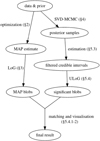 |
Fig. 1 High-level overview of our method for uncertainty-aware blob detection. |
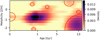 |
Fig. 2 Results of the LoG method (see Sect. 3) applied to the MAP estimate of the stellar distribution function. The detected blobs are indicated by red circles. |
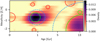 |
Fig. 3 Results of the proposed ULoG method to detect blobs with 95% credibility. The mock data and MAP estimate are the same as in Fig. 2. The significant blobs are visualised by dashed blue circles, their size corresponding to localisation uncertainty. Blobs in the MAP estimate that correspond to significant structures are marked in green, blobs that might be explainable by noise are marked in red (see Sect. 5.4.2). |
2 Problem setup
Our goal is to robustly identify distinct blobs in stellar population distribution functions by modelling integrated-light spectra. The distribution function f is a function of stellar metallicity z and age t, and it is physically constrained to be non-negative, i.e.

This can be related to an observed spectrum via simple stellar population (SSP) templates S (λ, z, t) which encode the spectra of single-age and single-metallicity stellar populations. The spectrum of a composite stellar population is a combination of SSPs weighted by f. Assuming that all stars in this composite population share a line-of-sight velocity distribution (LOSVD) ℒ(υ), then the observed spectrum is given by the composite rest-wavelength spectrum convolved by ℒ(υ). Putting this all together, the observation operator 𝒢 is given by
![$G\left( {f,L} \right) = \,\int {{{L\left( \upsilon \right)} \over {1 + {\upsilon \mathord{\left/ {\vphantom {\upsilon c}} \right. \kern-\nulldelimiterspace} c}}}\,\left[ {\int {\int {S\left( {{\lambda \over {1 + {\upsilon \mathord{\left/ {\vphantom {\upsilon c}} \right. \kern-\nulldelimiterspace} c}}},z,t} \right)f\left( {z,t} \right)\,{\rm{d}}t\,{\rm{d}}z} } } \right]\,{\rm{d}}\upsilon {\rm{.}}} $](/articles/aa/full_html/2023/06/aa44739-22/aa44739-22-eq2.png)
The observed data y are given by the addition of noise ϵ which is wavelength-dependent,

Since the goal of this work is to develop methods to robustly identify structures in f, we fix the LOSVD ℒ in our recoveries. Whilst Eqs. (1) and (2) relate continuous functions y, f and ℒ, in reality observations are made at a finite number of wavelengths λ. We therefore instead work with the discretised version of Eq. (2), for fixed ℒ, i.e.

Details of converting between continuous and discretised equations are in Sect. 2.1. The noise is typically assumed to be distributed as a multivariate normal with some covariance Σy,

where we assume that an estimate of Σy is available as is typically output from data-reduction pipelines. This completes the definition of our forward model. For the time being, we ignore several other physical ingredients which go into complete spectral models (e.g. LOSVD modelling, gas emission, reddening and calibration related continuum distortions). We discuss these effects further in Sect. 7.2.
Non-parametric recovery of f from noisy observations y is an ill-conditioned inverse problem. This means that noise in the observations is amplified in the recovery, leading to unrealistically spiky solutions. Solutions are found by minimising the mismatch between data and model as quantified by χ2,

The maximum likelihood (ML) solution is the one which minimises the χ2 mismatch, i.e.

To counter ill-conditioning, regularisation can be used to promote smoothness in the solution. In practice this means that rather than finding the ML solution, one instead finds the maximum a posteriori (MAP) solution by adding a penalty term to the objective function,

The penalty consists of a functional ℛ(f) which quantifies the smoothness of f multiplied by a tunable scalar β called the regularisation parameter. The functional is non-negative, and decreases for increasingly smooth f. When β = 0, the MAP and the ML solutions coincide, while in the limit of very large β, fMAP will be very smooth at the expense of no longer well reproducing the data. By appropriately tuning β to some intermediate value however the MAP solution will exhibit a good data-fit and a desired degree of smoothness. MAP recoveries are commonly used in stellar population modelling: Ocvirk et al. (2006) give a detailed description of the theory behind regularisation in this context, and it is available in the popular spectral modelling software Penalised Pixel-Fitting (pPXF, Cappellari 2017).
We will not address the question of how to tune the regularisation parameter β in this work. Several other suggestions have been made elsewhere. For example, the pPXF documentation1 offers the guideline to first perform an un-regularised fit, then increase β till the data mismatch increases to  where n is the size of the spectrum. Further well-known parameter choice rules are the L-curve method (Hansen & O’Leary 1993) and Morozov’s discrepancy principle (Groetsch 1983, provides a theoretical discussion). Alternative Bayesian approaches for choosing the regularisation parameter are discussed in Sect. 7.1. While the choice of regularisation parameter can affect the number of blobs visible in a recovered fMAP, in this work we restrict ourselves to the question of quantifying the uncertainty in the solution at fixed β and then using these uncertainty estimates to identify distinct blobs.
Regularisation can also be understood from a Bayesian perspective. Under this interpretation, Eq. (4) comes from the combination of a likelihood function

with a prior probability density function

Bayes’ theorem tells us that the posterior probability is proportional to the product of the likelihood and prior, i.e.

from which we can see that Eq. (4) picks out the solution fMAP which maximises the (log) posterior probability function. This is the origin of the name maximum a posteriori.
In this work, we assume a Gaussian prior on f that is truncated to the nonnegative orthant, since the density f cannot take negative values. That is, we make the choice

In the spirit of regularisation theory, we use the prior covariance Σf to encode smoothness assumptions on f (Calvetti & Somersalo 2018). Details on our choice for Σf are given in Sect. 2.1.
Viewed from this Bayesian perspective, we can explicitly see that regularisation incorporates prior information into the solution, and the regularisation parameter β controls the strength of the prior. Whilst a MAP solution may be considered Bayesian in the sense that it assumes a prior, it is nevertheless a single point estimate which on its own provides no information about uncertainty of the solution. In this work, we will introduce an efficient method to estimate this uncertainty based on dimensionality-reduced MCMC sampling.
The use of regularisation complicates another question commonly faced in stellar population modelling: the choice of whether to reconstruct mass-weighted or light-weighted quantities. These are two options for the parametrisation of f connected to the normalisation of SSP templates S in Eq. (1). If the SSPs are normalised to represent the flux of a unit mass of stars, f is said to be mass-weighted. In this case, the integrated flux of a stellar population is given by

SSP integrated flux varies strongly with age and, to a lesser extent, metallicity (Fig. 4). As an alternative to mass-weighting, the SSP templates S in Eq. (1) may be normalised to all have the same integrated flux, in which case the recovery is said to be light-weighted. Maximum-likelihood mass-weighted and light-weighted solutions should be self-consistent in the sense that

This consistency does not hold for MAP solutions. That is to say, the decision to regularise mass-weighted or light-weighted f will affect the result.
We think there is no single objectively correct preference between regularised mass- or light-weighted recoveries. Physically, one may imagine a mass of gas converting to stars at a rate varying smoothly with time, whence regularised mass-weights might seem to be the preferred option. Given that integrated SSP flux varies smoothly with age and metallicity however (see Fig. 4), mass-weighted smoothness would also imply light-weighted smoothness. Whilst both options may be reasonably justified under physical considerations, we raise this discussion here since numerically the situation is more complicated. For the MCMC based uncertainty quantification method we will present in Sect. 4, we find that sampling a model with regularised mass-weights is numerically unstable; see that section for further details. In order to facilitate comparison between all methods presented in this work, we will therefore only consider regularised light-weighted recoveries throughout. We also remark that this choice can be interpreted as a “linear functional strategy” (see Anderssen 1986) for reducing the ill-posedness of the reconstruction.
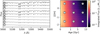 |
Fig. 4 Examples of SSP templates. Left panel shows 9 representative models from the MILES SSP library. These are labelled 1–9, corresponding to the position on the age-metallicity plane as shown in the right panel. The colourbar shows the integrated flux of the full grid of all 636 SSP templates as a function of age and metallicity. Younger stars are hotter and therefore brighter, explaining why integrated flux is a strong function of SSP age. Integrated flux depends more weakly on metallicity. For fixed age, we see that SSPs with greater metallicity have stronger absorption features e.g. compare spectra 7, 8 and 9 in the left panel. |
2.1 Discretisation
Here we outline the details of converting from continuous variables f, y, S etc. in Eq. (2), to the discretised version for a fixed LOSVD (Eq. (3)). We assume that data are available at n wavelengths
![${\bf{y}} = \,\left[ {y\left( {{\lambda _1}} \right), \ldots ,y\left( {{\lambda _n}} \right)} \right],$](/articles/aa/full_html/2023/06/aa44739-22/aa44739-22-eq16.png)
where typical values of n are around 1000. The domains of t and z can be discretised into T and Z intervals respectively. In practice, the age and metallicity discretisations are set by the choice of SSP library. The MILES library which we use has (Z, T) = (12, 53). We next introduce vectors gij equal to the SSP template of age ti and metallicity zi, pre-convolved by the (known) LOSVD, and multiplied by the discretisation interval widths, i.e.
![$\matrix{ {{{\bf{g}}_{ij}} = \left[ {{g_{ij}}\left( {{\lambda _1}} \right), \ldots ,{g_{ij}}\left( {{\lambda _n}} \right)} \right],} \hfill \cr {{g_{ij}}\left( \lambda \right) = {\rm{\Delta }}{t_i}{\rm{\Delta }}{z_j}\,\int {{{L\left( \upsilon \right)} \over {1 + {\upsilon \mathord{\left/ {\vphantom {\upsilon c}} \right. \kern-\nulldelimiterspace} c}}}S\left( {{\lambda \over {1 + {\upsilon \mathord{\left/ {\vphantom {\upsilon c}} \right. \kern-\nulldelimiterspace} c}}},{z_j},{t_j}} \right){\rm{d}}\upsilon .} } \hfill \cr } $](/articles/aa/full_html/2023/06/aa44739-22/aa44739-22-eq17.png)
Equation (2) now reduces to

This says that y is simply a sum of (pre-convolved) templates gij weighted by the 2D discretised distribution function fij, plus noise ϵ.
We correspondingly collect the templates gij into a 3D tensor G of shape (n, Z, T). Equation (7) can then be rewritten using tensor notation, i.e.

Corresponding to our choice to represent the image f as a matrix, the prior covariance Σf in (6) is given by a 4-tensor, where the entry Σfij,kl is equal to the covariance of the pixel intensities fij and fkl. As we remarked above, different choices for Σf correspond to different regularisation strategies. In this paper, we use the Ornstein-Uhlenbeck covariance

This choice corresponds to the intuitive assumption that neighbouring pixels in f are positively correlated, and that the amount of correlation decreases exponentially with distance. The parameter h > 0 is sometimes called the “correlation length”, as it controls the rate of this decrease.
2.2 Mock data
Throughout Sects. 3–5, we will use mock data to illustrate our methods. That is, we simulate a known ground truth LOSVD and distribution function f, apply the observation operator and add artificial noise to generate mock, noisy data. Here we describe the specific choices taken for these steps.
For the LOSVD we will use a fourth order Gauss–Hermite expansion (van der Marel & Franx 1993) which takes parameters

which correspond roughly to the mean, standard deviation, skewness and kurtosis of L(υ). We will generate mock-data using plausible galactic LOSVDs, namely using parameters θυ = [30, 100, −0.05, 0.1]. We fix θυ to the known ground truth during recoveries.
For the SSPs, we use the MILES2 models (Vazdekis et al. 2010) with BaSTI isochrones for base alpha-content (Pietrinferni et al. 2004) and a Chabrier (2003) initial mass function. These models span 53 ages in the range 0.03 < t/Gyr < 14 and 12 values of metallicity −2.27 < z/[M/H] < 0.4. Both age and metallicity values are non-uniformly spaced in these ranges. The overall 2D grid of SSP models consists of 636 template spectra. We use the wavelength range between [4700, 6500] Angstroms with a sampling in velocity space of 10 km s−1.
For the distribution functions we use random Gaussian mixtures. We generate ground-truth, light-weighted distributions f as mixtures of three Gaussian blobs which are randomly sized, shaped and positioned in the (non-uniformly spaced) age and metallicity domain shown for example in the right panel of Fig. 4. Specifically, the parameters describing the blobs are sampled in normalised co-ordinates which increase linearly from [0, 1] between the corners of the domain. Blob means are sampled uniformly between [0, 1]. The per-dimension variances are sampled independently from log-uniform distributions between [0.01, 1] and the blob covariance matrix is constructed using these variances and a random rotation. The blob weights are sampled from log-uniform distributions in the range [1, 30].
Finally, for the noise model we sample independent, normally distributed noise with a constant standard deviation σ2, i.e.

where σ is chosen so that the average signal-to-noise ratio (S/R) equals some specified value

Unless otherwise specified, we will use S/R = 100.
3 The Laplacian-of-Gaussians method for blob detection
In this section, we recall the necessary prerequisites on the Laplacian-of-Gaussians method. It is defined in terms of the Gaussian scale-space representation, which we introduce first.
3.1 The scale-space representation of an image
The scale-space representation of an image is a classic tool from computer vision, where it is used to study image structures at their intrinsic scale. For an exhaustive reference on scale-space theory in computer vision, see Lindeberg (1994).
A scale-space representation of a continuous image f : ℝ2 → ℝ is a one-parameter family (Lt)t≥0 of images with L0 = f, where the continuous parameter t ≥ 0 corresponds to physical scale. We will use the notation L(x, t) = Lt(x) to refer to the scale-space representation as a function both in x and t.
One distinguishes linear and non-linear scale space representations, where a scale space is called linear if, for all t ≥ 0, Lt is obtained from f by a linear operation, and else is called non-linear. The Gaussian scale space is arguably the most well-studied scale space, since it is the unique linear scale space that satisfies shift-invariance, scale invariance, the semigroup property and non-enhancement of local extrema (see Florack et al. 1992). It is defined as

where kt is a two-dimensional Gaussian of the form

3.2 The Laplacian-of-Gaussians method for blob detection
Given the Gaussian scale-space representation L of a continuous image f, the Laplacian-of-Gaussians (LoG) method (see Lindeberg 1998) detects blob-like image structures as the local minimisers and maximisers of the scale-normalised Laplacian of L, which is defined as

A local minimiser (x, t) ∈ ℝ2 × [0, ∞) of ΔnormL corresponds to a bright blob of scale t with centre x. On the other hand, local maximisers correspond to dark blobs. For the rest of this article, we will only consider the identification of bright blobs, since as explained in Sect. 1, we expect them to correspond to distinct stellar populations. While alternative ways to formally define blobs in an image have been studied (e.g. in Lindeberg 1994), those usually lead to less straightforward methods for detection. For the rest of this paper, we will always mean by a “blob” of an image fa local minimiser of ΔnormL. We note that the scale-normalisation in Eq. (10) is necessary to achieve scale-invariance of the detected interest points: If a blob of scale t is detected in the image f, then it should be detected as a blob of scale s · t in the rescaled image  .
.
To build some intuition on the LoG method, consider the prototypical Gaussian blob with scale parameter s and centre m:

It can then be shown that the scale-normalised Laplacian ΔnormL has exactly one local minimum at the point (x, t) = (m, s). Hence, we can recover the scale and centre of the Gaussian blob by determining the local minimum of ΔnormL in the 3-dimensional scale space. Furthermore, this corresponds to the intuition that blobs of an image correspond to points where the intensity of an image has highly negative or positive curvature, corresponding to structures that are bright or dark, respectively.
For a practical implementation, the LoG method has to be formulated for discrete images f ∈ ℝz×t and given a discrete set of scales 0 ≤ t1 < … < tK. Analogously to the continuous setting, the scale-space representation of a discrete image f is obtained from a discrete convolution,

As convolution kernel kt a sampled Gaussian is often used. However, this choice is not consistent with the scale-space axioms (see e.g. Sect. 1.2.2. in Weickert 1998), as discussed by Lindeberg (1990). Instead, the correct analogue of the continuous Gaussian kernel in the sense of scale-space theory has to be defined in terms of the modified Bessel function, i.e.


With this choice, the scale-space properties from the continuous setting hold exactly in the discrete setting (Lindeberg 1991). We have observed in our numerical tests that the use of this kernel leads to slightly better results than with the sampled Gaussian.
Given a discrete set of scales 0 ≤ t1 < … < tK, we obtain a discrete scale-space representation of the image f as three-dimensional matrix  . Similar to the continuous setting, blobs of the discrete image f are then detected as the local minimizers of
  , where Δnorm is the discrete scale-normalised Laplacian operator,

which is well-defined for all (i, j) ∈ {1, …, Z} × {1, …, T} by reflecting the image at the boundary. The numerical value of |ΔnormL| at a detected blob can be used as surrogate for the blob strength.
It is recommended to post-process the results of the LoG method by removing blobs that are too weak or overlap too much. First, all blobs for which the value of |ΔnormL| is below a certain threshold ltresh are removed. In the present work, we use a relative threshold of the form ltresh = rtresh · |min ΔnormLMAP|, where rtresh ∈ (0, 1). Without thresholding, the LoG method would detect blobs at the slightest fluctuations of the image intensity, which would often not correspond to meaningful features.
In a second step, the relative overlap of the detected blobs is computed. Hereby, a blob b = (i, j, q) is identified with a circle of radius  , centred at the pixel (i, j). If the relative overlap of two blobs surpasses a treshold
  , the blob with the smaller value of |ΔnormL| (i.e. the weaker blob) is removed.
We visualise a detected blob (i, j, t) by a circle centred at the pixel (i, j) and radius proportional to  . A common choice for the radius is
  , motivated by the fact that such a circle contains 68% of the total mass of a Gaussian with centre (i, j) and scale parameter t.
In Fig. 2, we plot the results of applying the LoG method to a MAP estimate of the stellar distribution function from mock data. In this particular case we used the relative threshold rthresh = 0.02 for the blob strength and the threshold othresh = 0.5 for the maximal relative overlap of two blobs.
Before we move on, we want to point out that while the postprocessing step is important, it should not be interpreted as a statistical procedure since it does not take the measurement error into account but only depends on the given point estimate of the distribution function. For example, a blob in the MAP estimate might be weak (i.e. a low value of |ΔnormL|) but its presence could be very certain. Vice versa, a very strong blob (|ΔnormL| large) in the estimate might at the same time be very uncertain.
4 An SVD-MCMC method for scalable uncertainty quantification
We wish to generalise the LoG method for blob detection to handle uncertainty. As a prerequiste to this, we first must explain how to quantify uncertainties for our problem. This poses some distinct challenges due to the combination of ill-posedness, high-dimensionality and non-negativity constraints, for which generic methods for uncertainty quantification are not well-suited.
In this section, we present a specialised MCMC method that is able to overcome the computational challenges in the reconstruction of stellar distribution functions. To make MCMC sampling computationally feasible for this problem we employ the following strategy: reduce the dimensions of the problem, sample the posterior in the reduced space, then deproject the solution back to the original space. The specific dimensionality reduction technique we will use is based on truncating the singular value decomposition (SVD) which is closely related to principal component analysis (PCA). This basic idea follows Tipping & Bishop (1999) however our method for deprojection is substantially different since we sample possible deprojections rather than take a single choice. In the context of stellar population modelling, previous work includes Falcón-Barroso & Martig (2021) who also combine SVD and MCMC sampling. Here, we build on this work by outlining how to deproject samples from the low-dimensional space in order to perform inference on stellar populations.
4.1 Notation
In this section, it will be useful to rewrite our model in a vectorised form, where we reshape 2D matrices to 1D vectors, 3D tensors to 2D matrices etc. Rather than introduce new baroque notation, for the duration of Sect. 4 we ask the reader to reinterpret existing notation in this fashion. Specifically, the forward model in Eq. (7), i.e.

originally had G as a 3D tensor of shape (n, Z, T) and f as the 2D image of shape (Z, T). Here we abuse notation and instead use f to refer to the 1D vectorised image of length Z · T and G to be correspondingly reshaped into a 2D matrix of shape (n, Z · T). Similarly the prior covariance Σf from Eq. (6) should now be considered a 2D covariance matrix rather than a 4-tensor.
4.2 SVD regression
The SVD is a matrix decomposition which generalises eigenvalue decomposition to rectangular matrices. For example, given a matrix G with shape (n, p = ZT), the SVD uniquely factorises G into three matrices,

The matrix S is a diagonal matrix whose entries are known as singular values, which are non-negative and are sorted in decreasing order (i.e. S[0, 0] ≥ S[1, 1] ≥ … ≥ 0). These are analogous to eigenvalues of an eigendecomposition. The columns of U and V contain orthonormal basis-vectors of the spaces ℝn and ℝp respectively, which are analogous to eigenvectors.
The SVD can be used for dimensionality reduction if the singular values decay sufficiently fast. The ‘truncated SVD’ retains only the first q components of the factorisation, i.e.
![$\matrix{ {{{\bf{U}}_q} = {\bf{U}}\left[ {:,:q} \right],} & {{{\bf{S}}_q} = {\bf{S}}\left[ {:q,:q} \right],} & {{{\bf{V}}_q} = {\bf{V}}} \cr } \,\left[ {:,:q} \right]. $](/articles/aa/full_html/2023/06/aa44739-22/aa44739-22-eq41.png)
The total squared-error incurred by approximating G by the truncated SVD is given by the sum of squares of the remaining p − q singular values, i.e.
![$\left\| {{\bf{G}} - {{\bf{U}}_q}{{\bf{S}}_q}{\bf{V}}_q^{\rm{T}}} \right\|_2^2 = \sum\limits_{i = q + 1}^p {{\bf{S}}{{\left[ {i,i} \right]}^2}.} $](/articles/aa/full_html/2023/06/aa44739-22/aa44739-22-eq42.png)
Therefore, if the singular values decay sufficiently fast then the truncated SVD can provide an accurate approximation of G for relatively small values of q. For the MILES SSP models (Vazdekis et al. 2010) we find that q = 15 provides a sufficiently good approximation. In general this choice will depend on the particular SSP models used and the data quality, and in Appendix B we suggest a general strategy to choose q.
The truncated SVD transforms our problem to a low-dimensional regression problem. We introduce the notation

and insert into Eq. (13) to give the transformed equation for the forward model,


The original p-dimensional parameter vector f in Eq. (13) has been reduced to a q-dimensional vector η in Eq. (16). To do inference on f, we first do inference on η using Eq. (16), then deproject back to infer f. Having reduced the dimensions and the condition-number of the problem, this problem is now computationally more amenable to MCMC sampling to estimate the posterior distribution p(η|y).
4.3 Deprojection
How should we perform the deprojection? The suggestion from Tipping & Bishop (1999) is to use the least-square deprojection of Eq. (17), i.e. for each sample η from the MCMC, calculate

This satisfies Eq. (17) because the SVD ensures that Vq is orthonormal (i.e.  ). The least-square deprojection is not suitable for our problem, however, since it is not guaranteed to satisfy the non-negativity constraint on f. In numerical tests, these deprojections did contain many negative entries and are therefore represent unphysical solutions. A solution to this problem would be to instead perform a constrained deprojection, where we minimise some function ℛ(f) subject to the desired constraints,

A natural choice for the function ℛ(f) is to use the same regularising penalty function defined in Eq. (4). For standard, quadratic choices of ℛ(f), Eq. (18) is a quadratic programming problem which can be solved efficiently. In practice, however, we find that this solution is unacceptable since these deprojections are unphysically spiky. Although the objective function in Eq. (18) promotes smoothness in the deprojections, the equality constraint  overwhelms this effect, resulting in unphysical deprojections too similar to the spiky ML solution.
The final strategy we investigated is to again use MCMC sampling. Whereas deprojection by calculating a point estimate will neglect uncertainty in the p–q SVD components which are not informed by the data, by sampling we can account for this. These components will instead be informed by the prior p(f) defined in Eq. (5), (i.e. the Bayesian equivalent of the regularisation term). Since the strength of this prior depends on a tunable regularisation parameter β, samples deprojected in this way can be made as smooth as desired, in analogy with MAP vs. ML recoveries.
4.4 SVD vs. PCA
SVD and PCA are closely related techniques. If we consider the matrix G to be a data matrix with n samples each of dimension p, and then we column-centre this matrix, i.e.
![${\bf{\hat G}} = {\bf{G}} - \left[ {{\bf{\mu }}, \ldots ,{\bf{\mu }}} \right]\,{\rm{where}}$](/articles/aa/full_html/2023/06/aa44739-22/aa44739-22-eq50.png)

and gi are the columns of G, then the SVD of  ,
,

is equivalent to PCA of the data. They are equivalent in the sense that the matrix  contains the principal axes of the data and the squares of the singular values in
  acquire the interpretation of being the variances explained by each principal component. In practice we find that using PCA works better than performing an SVD directly on G, so we adopt this choice throughout this work. We retain the name SVD-MCMC since the SVD interpretation helps to clarify the underlying ideas, and to prevent confusion with the more common usage of PCA as applied to observed spectra rather than model templates (e.g. Yip et al. 2004).
Centring G as in Eq. (19) transforms the forward model in Eq. (13) as follows,

where m is a scalar constant subject to the constraint

We define the truncated SVD of  equivalently to Eq. (14) to give
  ,
,  and
and  , then define
  equivalently to Eq. (15) to give the reduced forward model after PCA,

4.5 Probabilistic model and MCMC implementation
We can now define our probabilistic models and describe how we sample their posterior distributions. A probabilistic model is defined as a series of sampling statements and transformations of variables required to generate the observed data. Combined with Bayes’ theorem, the model implicitly defines an expression for the posterior probability function of the model unknowns given the observed data. An MCMC algorithm evaluates this expression to draw samples from the posterior.
We will compare two models, the Full MCMC model with no dimensionality reduction, and the SVD-MCMC model using the truncated SVD. Both models start by sampling the prior distribution on f, i.e.

The two models are:


In both cases, the final sampling statement draws data y from a multivariate normal with noise covariance Σy as defined in Eq. (9). Each model implicitly defines an expression for the posterior density p(f|y), which we sample via MCMC.
For MCMC sampling, we use the Hamiltonian Monte Carlo algorithm (HMC, Neal 2011) as implemented in the numpyro probabilistic programming language (Phan et al. 2019). Unless stated otherwise, for all experiments shown we run a single chain for 5000 warmup steps and 10000 sampling steps. The warmup parameters are left at the numpyro defaults. We check convergence with three criteria: (i) all sampled parameters have an  statistic (Gelman & Rubin 1992) in the range [0.95, 1.05], (ii) all sampled parameters have effective sample size (Geyer 2011) of at least 100, and (iii) no divergent transitions occur during sampling (Betancourt 2016).
Note that for the truncated SVD model, we directly sample the posterior p(f|y). That is, the deprojection occurs internally during sampling. We did also try the alternative implementation of first sampling p(η, m|y) and then later deprojecting as a subsequent step. The inferred posteriors and total computation times of the two implementations are very similar, however the first step of the alternative is orders of magnitude faster than the deprojection step. Modelling with SVD-truncated spectral templates is therefore an appealing option for purely kinematic models, where stellar populations can be considered as a nuisance effect and need not be deprojected. This is the approach taken by Falcón-Barroso & Martig (2021). If we do also wish to also perform inference over stellar populations, however, we see no clear benefit in separating the two sampling steps. Indeed, one possible downside to their separation is that sampling p(η, m|y) requires defining some arbitrary prior p(η, m). It is not possible for any such low-dimensional prior to be consistent with (21), or any physical prior, since the non-negativity constraint can only be satisfied in p-dimensions. Nevertheless, we note that both implementations of SVD-MCMC enjoys a significant speed-up compared to the full model.
5 Uncertainty-aware blob detection
How can we incorporate uncertainties into the LoG method for blob detection? Our motivation for doing so is demonstrated in Fig. 2: here we see that the LoG method identifies multiple blobs in the MAP estimate of the distribution function. However, the MAP estimate depends on the measurement noise, and so it is uncertain whether structures that are identified in this way also exist in the true, unknown stellar distribution function. Since this question needs to be addressed if one wants to make credible statements about the structure of the stellar distribution function, one has to find a way to incorporate the a-posteriori uncertainty of the stellar distribution function into the blob detection method.
In this section, we show how this can be achieved by combining the ideas from scale-space theory with the concept of multi-dimensional Bayesian credible intervals, a central tool for understanding and visualising uncertainty in imaging. This results in an uncertainty-aware variant of the Laplacian-of-Gaussians (LoG) method, which we correspondingly refer to as ULoG.
In Sect. 5.1, we will review Bayesian posterior credible intervals for images and related notions. In Sect 5.2, we introduce a new type of credible intervals that incorporates the notion of scale into the quantification of posterior uncertainty. We will refer to these as “filtered credible intervals”. Section 5.3 discusses how they can be estimated from MCMC samples. We then describe how filtered credible intervals can be used to define an uncertainty-aware variant of the Laplacian-of-Gaussians method, ULoG. The details of this method are given in Sect. 5.4.
5.1 Credible intervals for imaging
A central tool for Bayesian uncertainty quantification are “posterior credible intervals”. In general, they do not coincide with frequentist “confidence intervals” and should be interpreted differently. Since credible intervals are canonically only defined for scalar parameters, the definition has to be adapted when the unknown quantity of interest is multi-dimensional, as in the case of a discrete image.
Before we state the definition, it will be useful to introduce the following notation for multi-dimensional intervals: Let ℓ, u ∈ ℝz×t be two images such that ℓij ≤ uij for every pixel (i, j). Then, we will refer to the hyper-box
![$\left[ {{\bf{l}},{\bf{u}}} \right]: = \left\{ {{\bf{f}} \in {^{Z \times T}}:{\bf{l}} \le {\bf{f}} \le {\bf{u}}} \right\} \subset {^{Z \times T}}$](/articles/aa/full_html/2023/06/aa44739-22/aa44739-22-eq68.png)
as a multi-dimensional interval in ℝz×t. Given a posterior density function p(f|y) and a small credibility parameter α ∈ (0, 1), (typical values are α = 0.05 and α = 0.01, respectively representing 95%- and 99%-credibility), we then call a set [flow, fupp] ⊂ ℝZ×T a simultaneous (1 − α)-credible interval if
![$P\left( {{\bf{f}} \in \left[ {{{\bf{f}}^{{\rm{low}}}},{{\bf{f}}^{{\rm{upp}}}}} \right]\left| {\bf{y}} \right.} \right) \ge 1 - \alpha .$](/articles/aa/full_html/2023/06/aa44739-22/aa44739-22-eq69.png)
That is, the multi-dimensional interval [flow, fupp] contains at least a given percentage of the posterior probability mass. By looking at the plots of both the lower bound flow ∈ ℝz×t and the upper bound fupp ∈ ℝz×t, we can obtain a visual understanding of the posterior uncertainty. This is exemplified in the second row of Fig. 5. The first row shows a simulated ground truth from which mock data were generated (see Sect. 2.2). The second row shows the corresponding MAP estimate fMAP, together with the lower bound flow and upper bound fupp of simultaneous 95%-credible intervals.
Note that the simultaneous credible intervals defined in Eq. (23) have to be interpreted differently than ‘pixel-wise’ credible intervals which also appear in the statistical literature. We discuss these differences and the motivation behind our choice in Appendix A.
In Sect. 5.3, we describe how we compute simultaneous credible intervals using MCMC samples.
5.2 Filtered credible intervals
As a naive approach to perform uncertainty-aware blob detection we might try to identify the blobs directly from the simultaneous credible intervals. However, if the image of interest is highly uncertain, as is the case in the present problem of stellar recoveries, such an approach is rather limited. This can be seen from the first two rows of Fig. 5. One can observe that the MAP estimate is quite close to the ground truth. In contrast, the credible intervals are so wide that they only allow for very rough statements on the shape of the stellar distribution function. The lower bound is close to zero for most pixels. Clearly, the credible intervals alone do not accurately represent the quality of our estimate.
This problem can be resolved by recognising that we are less interested in the intensity values of specific pixels, but in higher-scale structures. Hence, we are actually interested in coarse-scale information. It is an important insight that – in contrast to the case where the image of interest is treated as given – the uncertainty with respect to higher scales cannot be directly derived from the uncertainties on finer scales. The correlation structure in the posterior distribution might be more complex and exhibit long-range dependencies, which means that the overall uncertainty cannot be reduced to the pixel-by-pixel case.
Consequently, if we want more informative uncertainty quantification, we have to integrate the notion of scale. This is achieved in our work by integrating the ideas of scale-space representations (see also Sect. 3.1): Instead of computing credible intervals for the vector of pixel intensities f, we can perform uncertainty quantification subject to a scale parameter t by computing credible intervals for the smoothed image Lt = kt * f, where kt is the discrete analogue of the Gaussian kernel, defined in Eqs. (11)–(12). That is, we compute images  such that
![$P\left( {{{\bf{L}}_t} \in \left[ {{\bf{L}}_t^{{\rm{low}}},{\bf{L}}_t^{{\rm{upp}}}} \right]\left| {\bf{y}} \right.} \right) \ge 1 - \alpha .$](/articles/aa/full_html/2023/06/aa44739-22/aa44739-22-eq71.png)
We will refer to [ as a filtered credible interval at scale t.
In the last three rows of Fig. 5, filtered credible intervals at three different scales are plotted. We see that the intervals tighten with increasing scale, but loose the ability to represent small structures. This visualises a very intuitive trade-off between scale and uncertainty: The uncertainty is lower with respect to larger (high-scale) structures, since they have less degrees of freedom. Correspondingly, the uncertainty with respect to small-scale structures is larger, as the given image has much more degrees of freedom at the small scale. The advantage of filtered credible intervals is that they allow for an explicit choice. If one is only interested in high-scale information, they allow to remove the superfluous uncertainty with respect to small-scale variations. If one moves to a finer scale, one has to pay the price of potentially larger uncertainty.
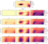 |
Fig. 5 Visualisation of credible intervals from mock data. The upper panel shows the ground truth from which the mock data were generated. In the second row, the MAP estimate fMAP (centre column) together with the lower bound flow (left) and upper bound fupp (right) of the (unfiltered) simultaneous credible intervals are plotted. Below that are the lower and upper bound of filtered credible intervals at 3 different scales, together with the corresponding filtered MAP estimate |

5.3 Estimating credible intervals from samples
Since in our case there are no analytical expressions for either unfiltered or filtered credible intervals, we have to estimate both using MCMC samples. After generating S samples f1, …, fS ∈ ℝz×T from the posterior distribution p(f|y), we estimate simultaneous (1 − α)-credible intervals [flow, fupp] by computing a multi-dimensional interval that contains the desired percentage of samples fi. That is, we find flow ∈ ℝz×t and fupp ∈ ℝz×t such that at least (1 − α) · S samples satisfy
![${{\bf{f}}^s} \in \left[ {{{\bf{f}}^{{\rm{low}}}},{{\bf{f}}^{{\rm{upp}}}}} \right].$](/articles/aa/full_html/2023/06/aa44739-22/aa44739-22-eq74.png)
Similarly, we estimate filtered credible intervals, at scale t, by computing a multi-dimensional interval that contains the desired percentage of filtered samples. That is, we find  such that at least (1 − α) · S samples satisfy
![${{\bf{k}}_t} * {{\bf{f}}^s} \in \left[ {{\bf{L}}_t^{{\rm{low}}},{\bf{L}}_t^{{\rm{upp}}}} \right].$](/articles/aa/full_html/2023/06/aa44739-22/aa44739-22-eq76.png)
In both cases, the estimation of credible intervals reduces to the following computational task: Given a sample of images x1, …, xS ∈ ℝz×t, find the smallest multi-dimensional interval [ℓ, u] ⊂ ℝz×t that contains at least (1 − α) · S of these samples (with xs = fs, this procedure estimates simultaneous credible intervals; with xs = kt * fs, this procedure estimates filtered credible intervals at scale t). This task is known as the k-enclosing box problem in computational geometry. We use the following heuristic but fast approach: First, find ℓ, u ∈ ℝZ×T such that for every pixel (i, j), there are at least (1 − α) · S images for which

(this is done using the order statistics of  . Since the resulting multi-dimensional interval [ℓ, u] usually contains too few points, it is then rescaled until it encloses at least (1 − α) · S points.
Note that there are several existing algorithms for solving the k-enclosing box problem exactly or approximately (see Segal & Kedem 1998; Chan & Har-Peled 2021). However, the computational complexity of these algorithms increases at least quadratically with the number of samples and exponentially with the underlying dimension, which renders them impractical for our high-dimensional problem. We also considered a classic method by Besag et al. (1995). However, in our numerical tests this method often led to credible intervals that contained 100% of the samples, rendering them useless. For our purposes, the heuristic approach was sufficient.
5.4 Uncertainty-aware Laplacian-of-Gaussians (ULoG)
In contrast to simultaneous credible intervals on the level of individual pixels, the filtered credible intervals in Fig. 5 show that there are some structures that are “significant”, in the sense that they are visible both in the image of the lower and the upper bound. This notion of significance is scale-dependent, since some structures might only be visible in the filtered credible intervals at sufficiently large scales. Intuitively, we would like to say that a blob is “credible” (at a given scale t) if all images ![$h \in \left[ {{\bf{L}}_t^{{\rm{low}}},{\bf{L}}_t^{{\rm{upp}}}} \right]$](/articles/aa/full_html/2023/06/aa44739-22/aa44739-22-eq79.png) exhibit a matching blob. Of course, one has to find a meaningful definition of what “matching” means, as the exact position and size of detectable blobs will usually vary among the images in
exhibit a matching blob. Of course, one has to find a meaningful definition of what “matching” means, as the exact position and size of detectable blobs will usually vary among the images in ![$\left[ {{\bf{L}}_t^{{\rm{low}}},{\bf{L}}_t^{{\rm{upp}}}} \right]$](/articles/aa/full_html/2023/06/aa44739-22/aa44739-22-eq80.png) . Since checking all these images is computationally infeasible, we instead define a suitable representative
. Since checking all these images is computationally infeasible, we instead define a suitable representative ![${{{\bf{\bar B}}}_t} \in \left[ {{\bf{L}}_t^{{\rm{low}}},{\bf{L}}_t^{{\rm{upp}}}} \right]$](/articles/aa/full_html/2023/06/aa44739-22/aa44739-22-eq81.png) that has “the least amount of blobs” in some quantitative sense. There are many different loss functions that penalise the amount of blobs in an image. We experimented with various loss functions of the form J(h) = ‖Dh‖2 with D being a discrete differential operator. Among all the differential operators we tested, the discrete Laplacian Δ led to the most favourable properties. We hence consider the representative
that has “the least amount of blobs” in some quantitative sense. There are many different loss functions that penalise the amount of blobs in an image. We experimented with various loss functions of the form J(h) = ‖Dh‖2 with D being a discrete differential operator. Among all the differential operators we tested, the discrete Laplacian Δ led to the most favourable properties. We hence consider the representative ![${{{\bf{\bar B}}}_t} \in \left[ {{\bf{L}}_t^{{\rm{low}}},{\bf{L}}_t^{{\rm{upp}}}} \right]$](/articles/aa/full_html/2023/06/aa44739-22/aa44739-22-eq82.png) given by the solution to the optimisation problem
given by the solution to the optimisation problem

This definition can be further motivated by the fact that in the LoG method, blobs are related to the local minima and maxima of the discrete Laplacian of an image (see Sect. 3.2). Hence, penalising  dampens the Laplacian and yields a feature-poor representative. On an intuitive level, solving (24) can be thought of as spanning a two-dimensional “blanket” between the lower bound
  and the upper bound
  . In accordance with this intuition, we will refer to the resulting image
  as a t-blanket. An image of a t-blanket generated from mock data is shown in Fig. 6.
To illustrate the intuition behind definition (24), a one-dimensional, continuous example is shown in Fig. 7. Given a MAP estimate fMAP : [0, 1] → ℝ of an unknown signal, assume that a posterior filtered credible interval is spanned by two functions ![$L_t^{{\rm{low}}}:\left[ {0,1} \right] \to {\rm{R}}$](/articles/aa/full_html/2023/06/aa44739-22/aa44739-22-eq88.png) and
and ![$L_t^{{\rm{upp}}}:\left[ {0,1} \right] \to {\rm{R}}$](/articles/aa/full_html/2023/06/aa44739-22/aa44739-22-eq89.png) . The t-blanket
. The t-blanket ![${{\bar B}_t}:\left[ {0,1} \right] \to {\rm{R}}$](/articles/aa/full_html/2023/06/aa44739-22/aa44739-22-eq90.png) is then the minimiser of ‖h″‖ over all functions h that satisfy the pointwise constraint
is then the minimiser of ‖h″‖ over all functions h that satisfy the pointwise constraint  and the boundary conditions h′(0) = h′(1) = 0. The blanket
  should not be confused with the filtered MAP estimate
  , which will in general be less smooth and might exhibit more blobs than
  , as seen in Fig. 7.
If we do not treat the scale t as given, we can study the three-dimensional scale-space structure of the “stack” of blankets  . We observed in numerical tests that any given blob will typically be visible in
  for a range of scales [t1, t2] ⊂ [0, ∞). At the lowest scale t1, it will typically be very weak, then grow stronger as the scale increases (and the uncertainty decreases, correspondingly) until it reaches a peak strength at some scale t*. Then, as the scale increases further towards t2, the strength of the blob decreases again as it is “smoothed out”. This phenomenon is somewhat analogous to the deterministic theory of scale-space blobs (see Lindeberg 1991). Motivated by this similarity, we consider the blanket stack
  as an “uncertainty-aware” scale-space representation. In a way, it represents our posterior uncertainty with respect to the unknown image f in scale space. In analogy to the LoG method from Sect. 3.2, we thus propose the heuristic principle that “significant” scale-space blobs correspond to local minimisers of
  in scale-space.
Instead of considering these significant blobs alone, we can obtain a more nuanced view of our information on the unknown stellar distribution by matching the set of candidate blobs detected in the MAP estimate fMAP (see e.g. Fig. 2) to the significant blobs detected from the blanket stack  . For example, if a blob is detected in the MAP but does not correspond to a significant blob in
  , it does not mean that it can be ignored, but only that its presence is too uncertain with respect to the given credibility level 1 − α.
In summary, we arrive at the following uncertainty-aware variant of the LoG method, which we refer to as ULoG. Given a discrete sequence of scales 0 ≤ t1 < … < tK, do the following:
Perform blob detection on the MAP estimate fMAP using the LoG method described in Sect. 3.2. Store the detected blobs in a set ℬ ⊂ {1, …, Z} × {1, …, T} × {1, …, K}.
-
For k = 1, …, K, do:
- (a)
Compute a filtered credible interval
![$\left[ {{\bf{L}}_{{t_q}}^{{\rm{low}}},{\bf{L}}_{{t_q}}^{{\rm{upp}}}} \right]$](/articles/aa/full_html/2023/06/aa44739-22/aa44739-22-eq106.png) .
. - (b)
Using
![$\left[ {{\bf{L}}_{{t_q}}^{{\rm{low}}},{\bf{L}}_{{t_q}}^{{\rm{upp}}}} \right]$](/articles/aa/full_html/2023/06/aa44739-22/aa44739-22-eq107.png) , compute the tq-blanket
, compute the tq-blanket  by solving Eq. (24).
- (a)
Stack the blankets in a 3-dimensional array
 .
.Determine the local minimisers of
 and store them in a set C.
Perform a matching procedure (see Sect. 5.4.1) that matches elements of ℬ to elements of C.
Visualise the results (see Sect. 5.4.2).
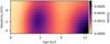 |
Fig. 6 Image of a t-blanket |

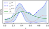 |
Fig. 7 Illustration of the idea behind definition (24). Given a filtered credible interval (shaded region) determined by a lower bound |


5.4.1 Matching procedure
We have not yet described the details of the matching procedure mentioned in the description of ULoG. There are of course many possibilities to define a criterion for blobs “matching”. For our purposes, the following procedure proved successful:
First, the detected blobs ℬ in the MAP estimate are post-processed, as described in Sect. 3.2. Which blobs remain in ℬ depends on the strength threshold lthresh and the overlap threshold
 .
.The scale-space minimisers C of
 are cleaned in the same way, the only difference being that ΔnormlMAP is replaced with
  .
.Now, for every b ∈ ℬ we check whether there is an overlap with any c ∈ C. Here, overlap is defined in the same way as in step (ii). If there exists a c ∈ C such that its relative overlap with b is above a threshold
 , then blobs b and c are a “match”.
The ideal configuration for the tunable parameters in this procedure will typically depend on the application. In our numerical experiments, we obtained satisfying results using lthresh = rthresh · |min ΔnormLMAP| with rthresh = 0.02 and  .
.
5.4.2 Visualisation
There are multiple ways in which we could visualise the results of the outlined algorithm. In Fig. 3, the following procedure was applied:
A scale-space blot) b = (i, j, q) is visualised as a circle with centre (i, j) and radius
 (see Sect. 3.2).
If a blob b ∈ ℬ does not match a blob in C, it is visualised as a red circle.
If a blob b ∈ ℬ matches a blob in C) it is visualised as a green circle. Furthermore, the match c is visualised as a dashed, blue circle.
The dashed blue circles have to be interpreted in the following way: If there is a second structure inside the circle, then we cannot distinguish it with confidence from the first blob. Hence, the radius of the circle indicates how well the blob can be localised for the given credibility level 1 − α. For example, in Fig. 3 we see that two blobs on the right correspond to the same blue circle. This means that we cannot separate them with credibility above 95%. We are confident that there is at least one blob in the true image f that corresponds to the blue circle, but we cannot say with credibility that there are two. Hence, these circles can be used as a tool to visualise localisation uncertainty in the blob detection.
6 Application to M 54
M 54 is the nuclear star cluster of the Sagittarius dwarf galaxy and hosts a mixture of stellar populations. Alfaro-Cuello et al. (2019) studied these populations using resolved data of individual stars in the cluster. They combined photometry from the Hubble Space Telescope with spectroscopic measurements from the Multi-Unit Spectroscopic Explorer (MUSE) to measure ages and metallicities of 6600 M 54 stars, whose distribution is shown in the top-left panel of Fig. 8. Two distinct clumps are clearly identifiable: an old metal-poor clump and young metal-rich clump, both of which display a trend of increasing metallicity for younger stars. The authors hypothesised that the old metal-poor population is formed from the accretion and merger of old and metal poor globular clusters, while the young population is some combination of stars formed in situ in M 54 and interlopers from the Sagittarius dwarf. We test our blob detection techniques on M 54, with these resolved measurements providing a ground truth distribution to compare with.
Boecker et al. (2020; hereafter B20) used the M54 MUSE data to compare age-metallicity recoveries from resolved measurements against those from integrated spectra. They created an integrated M 54 spectrum (S/R = 90) by co-adding the spectra of individual M 54 stars and analysed this using pPXF. The resulting recovery is shown in the upper right panel of Fig. 8. It matches the ground-truth distribution in coarse statistics, with mean age and metallicities from the two distributions separated by just 0.3 Gyr and 0.2 dex [Fe/H] respectively. The integrated recovery also displays distinct populations, well separated in age and metallicity. We see a young metal-rich population (single bright pixel at the top), and old metal-poor contributions also.
One further difference between the B20 result and the ground truth distribution is that the integrated recovery splits the old population into two clumps. The authors quantified the uncertainty in their pPXF recovery by Monte-Carlo resampling the data 100 times, randomly perturbed by the residual from the baseline pPXF fit. They calculated 100 MAP estimates from the resampled data, interpreting these as posterior samples. The pixel-wise 84% credible intervals of these samples enveloped the two clumps in the old population, suggesting that the split may not be significant. Our uncertainty-aware blob detection techniques are well placed to address this question in a principled way: our MCMC samples are directly drawn from the posterior, and ULoG is a well-motivated way to do blob detection using these samples. We therefore apply these techniques to the integrated M 54 spectrum from B20 to assess the significance of the recovered blobs.
6.1 Notes on the previous works
In the Alfaro-Cuello et al. (2019) resolved study, the authors dissect the metal-rich clump into two distinct populations. Whilst this extra split is supported by spatial and kinematic information (Alfaro-Cuello et al. 2020), based purely on the age-metallicity distribution seen in the upper left panel of Fig. 8 this split is not visible.
We noticed a small systematic effect in the B20 integrated-light study. In their recovery, a non-zero weight was assigned to the youngest SSP (0.03 Gyr) at an intermediate metallicity, with no counterpart in the resolved distribution. This very young contibution was not visible in the B20 paper since they use a linear axis for age, squashing very young SSPs to an inperceptably narrow range. Our visualisation – with a image pixel per SSP – highlighted this spurious contribution much more significantly. We believe this is a systematic effect. The spectra of the very youngest SSPs, hosting the hottest stars, are relatively featureless, showing relatively few and weak absorption features. A small contribution of very young stars may therefore be used to offset residuals from incorrect flux calibration and/or treatment for dust absorption. In order to focus our experiments on blobs with counterparts in the ground truth, we therefore exclude SSPs below 0.1 Gyr in our recoveries. After this cut, no weight is allocated to the youngest available SSP (i.e. 0.1 Gyr), supporting the hypothesis that this very young contribution was a systematic effect.
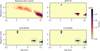 |
Fig. 8 Age-metallicity distributions for the M 54 star cluster. Top left: the ground truth number density from individual measurements of resolved stars in M 54, from Alfaro-Cuello et al. (2019). Top right: a MAP revovery using PPXF full spectrum fitting of an integrated-light M 54 spectrum, from B20. Bottom row: results of ULoG on M 54 data using low-regularisation. Both panels show the same MAP estimate of the recovered posterior probability density. The coloured circles show the location of significant blobs with 95%-credibility, with colours as in Fig. 3. The left shows results using SVD-MCMC, the right shows Full MCMC. In both cases, ULoG identifies 3 distinct blobs with 95%-credibility. |
6.2 Setup
The inputs for our recoveries mirror those used in B20. We use the same library of SSP templates (i.e. the Vazdekis et al. 2016 E-MILES library) with an bimodal IMF of slope 1.3, BaSTI isochrones (Pietrinferni et al. 2004) using all available metallicities, but only retaining ages above 0.1 Gyr (see Sect. 6.1). We mask the wavelengths ranges [5850, 5950], [6858.7–6964.9] and [7562.3-07695.6] (Angstrom) to avoid large sky-residuals. Since our analysis routines are specialised to the case of the purely linear part of spectral modelling, we first perform a fit with pPXF and fix the non-linear parts to the pPXF best-fit values. We find best fitting kinematic parameters of [V = 146 km s−1, σ = 3 km s−1, h3 = 0.088, h4 = 0.187] and the multiplicative polynomial of order 21 used by pPXF for continuum correction. We pre-process the SSP templates to account for these effects, convolving them with the LOSVD and multiplying them by the polynomial. Our Bayesian model was set up using a truncated Gaussian prior Eq. (6) with an Ornstein-Uhlenbeck covariance Eq. (8). The M 54 integrated spectrum and noise estimates were provided by the B20 authors. We try two choices for the regularisation parameter β: a low regularisation choice which gives a MAP reconstruction similar to the B20 result (β = 1 × 10³), and a high regularisation option for comparison (β = 5 × 10⁵).
We make the following specific choices for ULoG. To compute filtered credible intervals, we Full MCMC and SVD-MCMC with q = 15 (chosen as described in Appendix B). In both cases, we follow the procedure laid out in Sect. 4.5: taking 10000 samples for f and checking that convergence diagnostics are satisfied. To compute filtered credible intervals we consider 10 scales tk = 1 + (k − 1) · 1.5. The computation times (using Intel MKL on 8 3.6-GHz Intel Core i7-7700 CPUs and 64 GB RAM) were as follows: for low/high regularisation, SVD-MCMC required 1785/998 seconds, while Full MCMC required 12908/5295 seconds. This implies a speedup factor of roughly 5–10 for SVD-MCMC over the full model, with greater speedup for less regularisation.
6.3 Results
Fits to the data for the low-regularisation case are shown in Fig. 9. The residuals are smaller than 10%, showing that the data are well-fit. The fact that residuals are correlated between neighbouring wavelengths suggests inaccuracies at the 10% level in the assumed, uncorrelated noise model. The similarity between the SVD and Full-MCMC data-fits gives us confidence that the SVD truncation has not biased the results. The data fits for the high-regularisation case look very similar.
The recoveries for the low-regularisation case are shown in the bottom panels of Fig. 8. Results for both SVD-MCMC and Full MCMC again agree well. In both cases, ULoG detects three distinct blobs: one young and metal rich, and two old and metal poor. Importantly, we infer that these two old and metal poor blobs are not likely to be part of a single, combined blob. Justification for this can be seen clearly in Fig. 10 which shows marginalised constraints on the star formation histories: for old ages >5 Gyr, the 95% credible band are inconsistent with a single blob. For this level of regularisation, our computations clearly separate the old contribution into two metal-poor blobs whereas B20 does not. This conclusion strongly depends on the regularisation used, however.
Figures 11 and 12 show the inferred distributions using the high-regularisation option. Though the young and metal rich blob is still detected as significantly distinct, the two old and metal poor blobs have now merged together. Additionally, an insignificant blob (red circle) is now seen at an old and metal-rich population. The origin of this third blob is unclear, however it is not present when we extend the SSP grid to include younger ages. This is likely to be some systematic effect, however it is small and ultimately deemed statistically insignificant by ULoG. This detection of only two significant blobs more accurately matches the ground truth (top left panel of Fig. 8) which displays two rather than three distinct blobs. As with the low-regularisation case, in both Figs. 11 and 12 we see that the results of both SVD-MCMC and Full MCMC agree well. Thus, while our experiments have hopefully demonstrated the utility of ULoG (sped up with an SVD-MCMC backend) the dependence of blob detection on regularisation parameter remains an open question, which is discussed further in the next section.
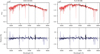 |
Fig. 9 Integrated M 54 spectrum y and the data fit ypred (in red), both for SVD-MCMC (left) and Full MCMC (right). The data fit is related to the respective MCMC posterior mean fmean through ypred = Gfmean. The plots in the second row show the relative residuals |

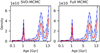 |
Fig. 10 Marginal posterior for the age distribution (see also Appendix A), for the low-regularisation case. We show 95%-credible intervals (shaded area) and marginal posterior mean (solid red line). Left: based on SVD-MCMC. Right: based on Full MCMC. |
7 Discussion
The ideas explained in Sect. 5 relate concepts from different fields such as mathematics, statistics and image processing. Since ULoG uses scale-space representations to perform statistical inference, it can be viewed as an example of a statistical scale-space method (see e.g. Holmström & Pasanen 2017). To our knowledge, the uncertainty-aware scale-space representation based on “blankets” (see Sect. 5.4) is new to the literature. Nevertheless, similar ideas have been used in variational imaging for a long time, although not in the context of uncertainty quantification, and are known as “taut string” or “tube methods” (see Mammen & van de Geer 1997; Davies & Kovac 2001; Hinterberger et al. 2003; Scherzer et al. 2009). Clarifying all of these connections is a promising starting point for theoretical work, since the resulting insights could be used to address various inference problems in astronomical imaging.
Our implementation of ULoG is based on SVD-MCMC (see Sect. 4). In this case, the overall computational cost of the method is dominated by the generation of posterior samples.
Given these samples, the additional cost of computing filtered credible intervals for a range of scales is negligible. Having access to posterior samples, one might also consider alternative ways to perform uncertainty-aware blob detection. One could try to circumvent the computation of filtered credible intervals altogether and instead apply the LoG method (or any other known blob detection algorithm) directly to each sample. However, such a direct approach has to tackle a number of challenges: First, there is no obvious way how to combine the results of the blob detection from each individual sample into meaningful statistics. Different samples might have blobs of widely differing size at non-matching locations. Furthermore, individual posterior samples tend to be quite noisy. This is problematic, since a blob detection method applied to a noisy sample will detect a large number of “spurious” blobs, making it very challenging to extract meaningful information from its result.
However, ULoG has the key advantage that it only requires computation of filtered credible intervals. This means that it does not explicitly need access to posterior samples and hence can be combined with any method of estimating filtered credible intervals. For example, in the context of linear imaging problems Pereyra (2017) proposed to estimate posterior credible regions using concentration-inequalities, circumventing the need for sampling. Approaches based on this idea have been shown to be very scalable (see e.g. Cai et al. 2018a). Using concentration-inequalities to directly estimate filtered credible intervals could make ULoG applicable to very large imaging problems. We will investigate this idea in future work.
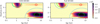 |
Fig. 11 Results of ULoG on M 54 data with higher regularisation. |
7.1 SVD-MCMC
We have seen in Sect. 6 that the choice of the regularisation parameter β in Eq. (5) affects the inferences. There are various strategies to address the choice of β in the Bayesian framework, which would be straightforward to combine with SVD-MCMC. In a hierarchical approach (see e.g. Molina et al. 1999; Pereyra et al. 2015), we could assign a prior on β. Alternatively, we could estimate β from the data using empirical Bayesian methods (e.g. as in Pereira et al. 2015; Vidal et al. 2020). We could also try to eliminate the presence of the regularisation parameter altogether, and use a simulation-based prior (for an example in the context of weak gravitational lensing, see Remy et al. 2023).
While in this paper we implemented SVD-MCMC with HMC, one could consider different MCMC methods. For example, SVD-MCMC could be combined with specialised samplers for nonsmooth probability densities, such as proximal MCMC (Durmus et al. 2018) for example, to allow the use of ℓ1-Laplace priors, which is a common choice in imaging (see e.g. Caselles et al. 2015).
In our numerical tests, we observed that the HMC sampler ran into numerical problems when the regularising prior was assigned to f in mass-weights instead of light-weights. Specifically, a significant number of divergent transitions occurred (Betancourt 2016), and  statistics were much greater than 1, signalling unconverged chains. This is likely due to the fact that the observation operator 𝒢 is much more ill-conditioned with respect to mass-weighted distribution functions. This problem could be resolved by replacing HMC with a more robust sampler, such as Randomize-Then-Optimize (Bardsley et al. 2014) for example, though it is unclear how efficient this specific option would be for such a high-dimensional problem.
7.2 Applications beyond the current problem
In this work, we have presented ULoG and SVD-MCMC on an idealised problem. Several other effects may be important for spectral modelling, including convolution with the LOSVD, treatment for reddening, and accounting for gas emission. For the M 54 experiment presented here, we have pre-processed the data to remove these effects before proceeding with the linear stellar population model. We note that in the future, these other effects could be incorporated into a more complete model which is still fully compatible with SVD-MCMC and ULoG.
Our method for uncertainty-aware blob detection is very general and may find applications beyond spectral modelling. One specific example which we intend to explore in the future is the task of blob detection in orbit distributions inferred from orbit-super position modelling of galaxies (e.g. Zhu et al. 2022).
In our application to M 54, we have seen that SVD-MCMC can lead to a reduction of computation time up to a factor 7 compared to Full MCMC. For larger problems, this factor might even increase as the full potential of the truncated SVD comes truly into play in higher dimensions. Potentially, this could make uncertainty quantification feasible not only for single-spectrum fitting, but even for full IFU datacube modelling (see e.g. Hinterer et al. 2023).
8 Conclusions
In this work, we have adressed the question of blob detection in images with uncertainties. We have proposed a novel, uncertainty-aware variant of the classic Laplacian-of-Gaussians method for blob detection (ULoG). ULoG detects significant blobs considering various scales, and requires as input uncertainty estimates for the image in the form of filtered credible intervals. Furthermore, we describe an efficient computational method for calculating filtered credible intervals which combines truncated SVD and MCMC sampling (SVD-MCMC).
These methods have been developed in the context of stellar population modelling of integrated-light spectra. We illustrated the methods first on mock data, and then applied it to real data of the nuclear star cluster M 54. Results using SVD-MCMC and Full MCMC match well. The observed speed-up using SVD-MCMC is on average a factor 7, with sampling lasting 15–30 min as opposed to 2–4 h. The number of significant blobs detected ranged between 2 and 3, depending on the amount of regularisation used. This work focussed on uncertainty-aware blob detection at fixed regularisation, but in the future our methods can be combined with Bayesian techniques for selecting or marginalising over the regularisation parameter.
Acknowledgements
The authors thank the referee for a constructive and helpful report. P.J. and G.vdV. acknowledge funding from the European Research Council (ERC) under the European Union’s Horizon 2020 research and innovation programme under grant agreement No 724857 (Consolidator Grant ArcheoDyn). PJ and GvdV also acknowledge support by the Austrian Science Fund (FWF): F6811-N36. FP and OS were funded by the Austrian Science Fund (FWF): F6807-N36. The financial support by the Austrian Federal Ministry for Digital and Economic Affairs, the National Foundation for Research, Technology and Development and the Christian Doppler Research Association is gratefully acknowledged. AB was funded by the Deutsche Forschungsgemeinschaft (DFG, German Research Foundation) – Project-ID 138713538 – SFB 881 (“The Milky Way System”, subproject B08) and acknowledges support from grant ProID2021010080 in the framework of Proyectos de I+D por organismos de investigación y empresas en las áreas prioritarias de la estrategia de especialización inteligente de Canarias (RIS-3), FEDER Canarias 2014-2020.
Appendix A Simultaneous vs. pixel-wise credible intervals
In section 5.1 we defined credible intervals as simultaneous intervals. These need to be distinguished from pixel-wise credible intervals that are also often used for uncertainty visualisation (for scalar parameters, these notions coincide). Given a pixel (i, j), we call an interval [ℓij, uij] ⊂ ℝ a pixel-wise posterior (1 − α)-credible interval if it is a (1 − α)-credible interval with respect to the marginalised posterior distribution p(fij|y). That is, if there holds
![$P\left( {{f_{ij}} \in \left[ {{\ell _{ij}},{u_{ij}}} \right]\left| {\bf{y}} \right.} \right) \ge 1 - \alpha .$](/articles/aa/full_html/2023/06/aa44739-22/aa44739-22-eq119.png)
If we assemble all lower bounds (ℓij) and upper bounds (uij) into images ℓ, u ∈ ℝT×Z, these images define then a multidimensional interval [ℓ, u] ⊂ ℝT×Z via equation (22). However, this interval will in general not satisfy equation (23), as pointed out e. g. by Ganesh (2009). For our purposes, simultaneous credible intervals are more suitable, since by definition they satisfy equation (23), thus allowing the intuitive interpretation that the signal of interest lies “between” the lower bound f1ow and the upper bound fupp with posterior probability greater or equal 1 − α.
The difference between simultaneous and pixel-wise credible intervals can also be stated by referring to the concept of posterior credible regions. We call a set Cα ⊂ ℝT×Z a posterior (1 − α)-credible region for f if

By equation (23), a simultaneous (1 − α)-credible interval is always a (1 − α)-credible region, while this might fail for a pixel-wise (1 − α)-credible interval.
We also remark that the terminology in this area is not completely standardised. Credible regions and credible intervals are sometimes called Bayesian confidence regions and Bayesian confidence intervals, respectively, while the multi-dimensional simultaneous credible intervals mentioned above have been referred to as Bayesian confidence bands or credible bands in the area of time series analysis (see Breth 1978).
Credible intervals for the age distribution
The credible intervals for the age distribution plotted in figures 10 and 12 were computed as follows: For each MCMC sample fs, we sum over the metallicity,

Then, we estimated simultaneous 95%-credible intervals for a ∈ ℝT using the method outlined in section 5.3 (that is, setting xs = as).
Appendix B Choice of q
How can we choose an appropriate size of the latent dimension q? One possibility is to look at the rate of decay of singular values. These are shown for our problem in the top panel of Figure B.1. Singular values decay more slowly beyond q = 15, hence the accuracy of the truncated SVD approximation grows more slowly beyond this value. Choosing a value of q around this inflection point provides a good balance between accuracy and possible speed-up from dimensionality reduction. Note however that this choice is not guaranteed to be sufficient in all circumstances. For very high signal-to-noise data, for example, it is conceivable that a larger q may be required. We therefore recommend to check convergence of results against the choice q.
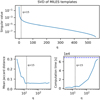 |
Fig. B.1 Influence of the latent dimension q on SVD-MCMC. The top panel shows singular values of the matrix of MILES SSPs. The lower left panel shows the error between filtered credible intervals computed with SVD-MCMC and Full MCMC. The error is measured in the mean Jaccard distance (see equation (B.1)). Beyond q = 15 the error stabilises, signalling converged results. The lower right panel shows the corresponding computation time for SVD-MCMC, where the dashed horizontal line marks the computation time for Full MCMC. In all panels, the vertical dotted line is at q = 15, the value adopted for SVD-MCMC inferences in this work. |
To assess convergence we will run SVD-MCMC over a range of q and quantify changes in the results. The metric we will use to compare two sets of MCMC samples is the mean Jaccard distance between filtered credible intervals computed from the samples. For two intervals [u1, υ1], [u2, υ2] ⊂ ℝ, we define their Jaccard distance as
![${D_J}\left( {\left[ {{u^1},{\upsilon ^1}} \right],\left[ {{u^2},{\upsilon ^2}} \right]} \right) = 1 - {{\left| {\left[ {{u^1},{\upsilon ^1}} \right] \cap \left[ {{u^2},{\upsilon ^2}} \right]} \right|} \over {\left| {\left[ {{u^1},{\upsilon ^1}} \right] \cup \left[ {{u^2},{\upsilon ^2}} \right]} \right|}}.$](/articles/aa/full_html/2023/06/aa44739-22/aa44739-22-eq122.png)
The value of the Jaccard distance is always between 0 and 1, where 0 corresponds to identity and 1 corresponds to disjointness (up to sets of measure zero). To measure the distance between filtered credible intervals [u1, υ1], [u2, υ2] ⊂ ℝt×z in image space, we take the mean Jaccard distance over all pixels:
![${\bar D_J}\left( {\left[ {{{\bf{u}}^1},{{\bf{\upsilon }}^1}} \right],\left[ {{{\bf{u}}^2},{{\bf{\upsilon }}^2}} \right]} \right): = {1 \over {T \cdot Z}}\sum\limits_{i = 1}^T {\sum\limits_{j = 1}^Z {{D_J}\left( {\left[ {u_{ij}^1,\upsilon _{ij}^1} \right],\left[ {u_{ij}^2,\upsilon _{ij}^2} \right]} \right).} } $](/articles/aa/full_html/2023/06/aa44739-22/aa44739-22-eq123.png)
The lower left panel of figure B.1 shows the results of our convergence test on mock data. It shows the mean Jaccard distance between filtered credible intervals computed using Full MCMC and SVD-MCMC with 5000 warmup and 5000 sampling steps as a function of q. The filtered credible intervals were computed for scale t = 5 and credibility parameter α = 0.05, but we observed that the choice of these parameters did not significantly affect the resulting plot. Beyond q = 15 the distance does not decrease, signalling that filtered credible intervals do not systematically change and our results are converged. The minimum distance does not reach zero, but instead flattens around 0.05 due to the inherent stochasticity of samples (i.e. two independent sets of samples from the Full MCMC model would also show this level of difference). The bottom right panel of figure B.1 shows the computation time required for sampling the SVD-MCMC models as a function of q. At q = 15, we still benefit from a factor 15 speedup compared to sampling the full model.
For general usage of SVD-MCMC (where it may be infeasible or undesirable to compare against Full MCMC), we suggest the following strategy for picking q. Pick some initial q0 smaller than the inflection point of the singular values and a step-size Δq ≈ 5. Perform SVD-MCMC inferences at q = q0 + iΔq, first for i = 0 and 1, and compute the Jaccard distance between these two sets of results. If q0 is small enough, there will likely be a significant decrease in Jaccard distance between i = 0 and 1. Finally, increment i, computing the Jaccard distance between the cases i and i − 1, till the distance stabilises to a constant value.
References
- Alfaro-Cuello, M., Kacharov, N., Neumayer, N., et al. 2019, ApJ, 886, 57 [Google Scholar]
- Alfaro-Cuello, M., Kacharov, N., Neumayer, N., et al. 2020, ApJ, 892, 20 [CrossRef] [Google Scholar]
- Anderssen, R. S. 1986, in Inverse Problems: Proceedings of the Conference Held at the Mathematical Research Institute at Oberwolfach, eds. J. R. Cannon, & U. Hornung (Birkhäuser Basel), 11 [Google Scholar]
- Bardsley, J. M. 2012, SIAM J. Sci. Comput., 34, A1316 [CrossRef] [Google Scholar]
- Bardsley, J. M., Solonen, A., Haario, H., & Laine, M. 2014, SIAM J. Sci. Comput., 36, A1895 [NASA ADS] [CrossRef] [Google Scholar]
- Besag, J., Green, P., Higdon, D., & Mengersen, K. 1995, Stat. Sci., 10 [Google Scholar]
- Betancourt, M. 2016, arXiv e-prints, [arXiv: 1604.00695] [Google Scholar]
- Boecker, A., Alfaro-Cuello, M., Neumayer, N., Martín-Navarro, I., & Leaman, R. 2020, ApJ, 896, 13 [NASA ADS] [CrossRef] [Google Scholar]
- Breth, M. 1978, Ann. Stat., 6, 649 [CrossRef] [Google Scholar]
- Cai, X., Pereyra, M., & McEwen, J. D. 2018a, MNRAS, 480, 4170 [NASA ADS] [CrossRef] [Google Scholar]
- Cai, X., Pereyra, M., & McEwen, J. D. 2018b, MNRAS, 480, 4154 [NASA ADS] [CrossRef] [Google Scholar]
- Calvetti, D., & Somersalo, E. 2018, Wiley Interdiscip. Rev. Comput. Stat., 10, e1427 [CrossRef] [Google Scholar]
- Cappellari, M. 2017, MNRAS, 466, 798 [Google Scholar]
- Cappellari, M., & Emsellem, E. 2004, PASP, 116, 138 [Google Scholar]
- Carnall, A. C., McLure, R. J., Dunlop, J. S., & Davé, R. 2018, MNRAS, 480, 4379 [Google Scholar]
- Caselles, V., Chambolle, A., & Novaga, M. 2015, in Handbook of Mathematical Methods in Imaging, 3 [Google Scholar]
- Chabrier, G. 2003, PASP, 115, 763 [Google Scholar]
- Chan, T. M., & Har-Peled, S. 2021, Discrete Comput. Geom., 66, 769 [CrossRef] [Google Scholar]
- Cid Fernandes, R., Mateus, A., Sodré, L., Stasinska, G., & Gomes, J. M. 2005, MNRAS, 358, 363 [CrossRef] [Google Scholar]
- Dashti, M., & Stuart, A. M. 2017, in Handbook of Uncertainty Quantification, eds. R. Ghanem, D. Higdon, & H. Owhadi (Springer International Publishing), 311 [CrossRef] [Google Scholar]
- Davies, P. L., & Kovac, A. 2001, Ann. Stat., 29, 1 [Google Scholar]
- Despali, G., Vegetti, S., White, S. D. M., et al. 2022, MNRAS, 510, 2480 [NASA ADS] [CrossRef] [Google Scholar]
- Durmus, A., Moulines, É., & Pereyra, M. 2018, SIAM J. Imaging Sci., 11, 473 [CrossRef] [Google Scholar]
- Falcón-Barroso, J., & Martig, M. 2021, A & A, 646, A31 [CrossRef] [EDP Sciences] [Google Scholar]
- Florack, L. M. J., ter Haar Romeny, B. M., Koenderink, J. J., & Viergever, M. A. 1992, Image Vis. Comp., 10, 376 [Google Scholar]
- Ganesh, N. 2009, J. Multivar. Anal., 100, 1610 [Google Scholar]
- Gelman, A., & Rubin, D. B. 1992, Stat. Sci., 7, 457 [Google Scholar]
- Geyer, C. J. 2011, in Handbook of Markov Chain Monte Carlo (London New York: CRC Press) [Google Scholar]
- Gladders, M. D., Oemler, A., Dressler, A., et al. 2013, ApJ, 770, 64 [NASA ADS] [CrossRef] [Google Scholar]
- Groetsch, C. W. 1983, in Improperly Posed Problems and Their Numerical Treatment, eds. G. Hämmerlin, & K.-H. Hoffmann, International Series of Numerical Mathematics (Birkhäuser), 97 [CrossRef] [Google Scholar]
- Hansen, P. C., & O’Leary, D. P. 1993, SIAM J. Sci. Comput., 14, 1487 [NASA ADS] [CrossRef] [Google Scholar]
- Hanson, K. M. 1993, in Medical Imaging 1993: Image Processing, 1898, ed. M. H. Loew (SPIE), 716 [Google Scholar]
- Hinterberger, W., Hintermüller, M., Kunisch, K., von Oehsen, M., & Scherzer, O. 2003, J. Math. Imaging Vis., 19, 219 [CrossRef] [Google Scholar]
- Hinterer, F., Hubmer, S., Jethwa, P., et al. 2023, SIAM J. Imaging Sciences, 16, 192 [CrossRef] [Google Scholar]
- Holmström, L., & Pasanen, L. 2017, Int. Stat. Rev., 85, 1 [CrossRef] [Google Scholar]
- Kaipio, J., & Somersalo, E. 2007, J. Comput. Appl. Math., 198, 493 [NASA ADS] [CrossRef] [Google Scholar]
- Koleva, M., Prugniel, P., Ocvirk, P., Le Borgne, D., & Soubiran, C. 2008, MNRAS, 385, 1998 [NASA ADS] [CrossRef] [Google Scholar]
- Leja, J., Carnall, A. C., Johnson, B. D., Conroy, C., & Speagle, J. S. 2019, ApJ, 876, 3 [Google Scholar]
- Li, Y., Wang, S., Tian, Q., & Ding, X. 2015, Neurocomputing, 149, 736 [CrossRef] [Google Scholar]
- Lindeberg, T. 1990, IEEE Trans. Pattern Anal. Mach. Intell., 12, 234 [CrossRef] [Google Scholar]
- Lindeberg, T. 1991, PhD thesis, Royal Institute of Technology, Stockholm and Stockholm University [Google Scholar]
- Lindeberg, T. 1994, Scale-Space Theory in Computer Vision (Boston: Springer) [CrossRef] [Google Scholar]
- Lindeberg, T. 1998, Int. J. Comput. Vis., 30, 79 [Google Scholar]
- Lindeberg, T. 2013, J. Math. Imaging Vis., 46, 177 [CrossRef] [Google Scholar]
- Lower, S., Narayanan, D., Leja, J., et al. 2020, ApJ, 904, 33 [NASA ADS] [CrossRef] [Google Scholar]
- Mammen, E., & van de Geer, S. 1997, Ann. Stat., 25, 387 [Google Scholar]
- Martin, J., Wilcox, L. C., Burstedde, C., & Ghattas, O. 2012, SIAM J. Sci. Comput., 34, A1460 [NASA ADS] [CrossRef] [Google Scholar]
- Masias, M., Freixenet, J., Lladó, X., & Peracaula, M. 2012, MNRAS, 422, 1674 [NASA ADS] [CrossRef] [Google Scholar]
- Mikolajczyk, K., Tuytelaars, T., Schmid, C., et al. 2005, Int. J. Comput. Vis., 65, 43 [CrossRef] [Google Scholar]
- Molina, R., Katsaggelos, A., & Mateos, J. 1999, IEEE Trans. Image Process., 8, 231 [CrossRef] [Google Scholar]
- Neal, R. 2011, in Handbook of Markov Chain Monte Carlo, 113 [Google Scholar]
- Ocvirk, P., Pichon, C., Lançon, A., & Thiébaut, E. 2006, MNRAS, 365, 46 [Google Scholar]
- Parno, M., Davis, A., & Seelinger, L. 2021, JOSS, 6, 3076 [NASA ADS] [CrossRef] [Google Scholar]
- Pereira, A., Antoni, J., & Leclère, Q. 2015, Appl. Acoust., 97, 11 [CrossRef] [Google Scholar]
- Pereyra, M. 2017, SIAM J. Imaging Sci., 10, 285 [CrossRef] [Google Scholar]
- Pereyra, M., Bioucas-Dias, J. M., & Figueiredo, M. A. T. 2015, in 2015 23rd European Signal Processing Conference (EUSIPCO), 230 [CrossRef] [Google Scholar]
- Phan, D., Pradhan, N., & Jankowiak, M. 2019, arXiv preprint [arXiv:1912.11554] [Google Scholar]
- Pietrinferni, A., Cassisi, S., Salaris, M., & Castelli, F. 2004, ApJ, 612, 168 [Google Scholar]
- Price, M. A., Cai, X., McEwen, J. D., et al. 2020, MNRAS, 492, 394 [Google Scholar]
- Price, M. A., McEwen, J. D., Cai, X., et al. 2021, MNRAS, 506, 3678 [NASA ADS] [CrossRef] [Google Scholar]
- Remy, B., Lanusse, F., Jeffrey, N., et al. 2023, A & A, 672, A51 [NASA ADS] [CrossRef] [EDP Sciences] [Google Scholar]
- Repetti, A., Pereyra, M., & Wiaux, Y. 2018, in 2018 26th European Signal Processing Conference (EUSIPCO), 2668 [CrossRef] [Google Scholar]
- Scherzer, O., Grasmair, M., Grossauer, H., Haltmeier, M., & Lenzen, F. 2009, Variational Methods in Imaging (Springer) [Google Scholar]
- Segal, M., & Kedem, K. 1998, Inf. Process. Lett., 65, 95 [CrossRef] [Google Scholar]
- Simha, V., Weinberg, D. H., Conroy, C., et al. 2014, arXiv e-prints, [arXiv: 1484.8482] [Google Scholar]
- Tipping, M. E., & Bishop, C. M. 1999, J. R. Stat. Soc., B: Stat. Methodol., 61, 611 [CrossRef] [Google Scholar]
- Tojeiro, R., Heavens, A. F., Jimenez, R., & Panter, B. 2007, MNRAS, 381, 1252 [NASA ADS] [CrossRef] [Google Scholar]
- van der Marel, R. P., & Franx, M. 1993, ApJ, 407, 525 [Google Scholar]
- Vazdekis, A., Sánchez-Blázquez, P., Falcón-Barroso, J., et al. 2010, MNRAS, 404, 1639 [NASA ADS] [Google Scholar]
- Vazdekis, A., Coelho, P., Cassisi, S., et al. 2015, MNRAS, 449, 1177 [Google Scholar]
- Vazdekis, A., Koleva, M., Ricciardelli, E., Röck, B., & Falcón-Barroso, J. 2016, MNRAS, 463, 3409 [Google Scholar]
- Vidal, A. F., De Bortoli, V., Pereyra, M., & Durmus, A. 2020, SIAM J. Imaging Sci., 13, 1945 [CrossRef] [Google Scholar]
- Weickert, J. 1998, Anisotropic Diffusion in Image Processing (Stuttgart: B. G. Teubner) [Google Scholar]
- White, S. D. M., & Rees, M. J. 1978, MNRAS, 183, 341 [Google Scholar]
- Yip, C. W., Connolly, A. J., Vanden Berk, D. E., et al. 2004, AJ, 128, 2603 [Google Scholar]
- Zhu, L., van de Ven, G., Leaman, R., et al. 2022, A & A, 664, A115 [Google Scholar]
All Figures
|
Fig. 1 High-level overview of our method for uncertainty-aware blob detection. |
| In the text | |
|
Fig. 2 Results of the LoG method (see Sect. 3) applied to the MAP estimate of the stellar distribution function. The detected blobs are indicated by red circles. |
| In the text | |
|
Fig. 3 Results of the proposed ULoG method to detect blobs with 95% credibility. The mock data and MAP estimate are the same as in Fig. 2. The significant blobs are visualised by dashed blue circles, their size corresponding to localisation uncertainty. Blobs in the MAP estimate that correspond to significant structures are marked in green, blobs that might be explainable by noise are marked in red (see Sect. 5.4.2). |
| In the text | |
|
Fig. 4 Examples of SSP templates. Left panel shows 9 representative models from the MILES SSP library. These are labelled 1–9, corresponding to the position on the age-metallicity plane as shown in the right panel. The colourbar shows the integrated flux of the full grid of all 636 SSP templates as a function of age and metallicity. Younger stars are hotter and therefore brighter, explaining why integrated flux is a strong function of SSP age. Integrated flux depends more weakly on metallicity. For fixed age, we see that SSPs with greater metallicity have stronger absorption features e.g. compare spectra 7, 8 and 9 in the left panel. |
| In the text | |
|
Fig. 5 Visualisation of credible intervals from mock data. The upper panel shows the ground truth from which the mock data were generated. In the second row, the MAP estimate fMAP (centre column) together with the lower bound flow (left) and upper bound fupp (right) of the (unfiltered) simultaneous credible intervals are plotted. Below that are the lower and upper bound of filtered credible intervals at 3 different scales, together with the corresponding filtered MAP estimate |
| In the text | |
|
Fig. 6 Image of a t-blanket |
| In the text | |
|
Fig. 7 Illustration of the idea behind definition (24). Given a filtered credible interval (shaded region) determined by a lower bound |
| In the text | |
|
Fig. 8 Age-metallicity distributions for the M 54 star cluster. Top left: the ground truth number density from individual measurements of resolved stars in M 54, from Alfaro-Cuello et al. (2019). Top right: a MAP revovery using PPXF full spectrum fitting of an integrated-light M 54 spectrum, from B20. Bottom row: results of ULoG on M 54 data using low-regularisation. Both panels show the same MAP estimate of the recovered posterior probability density. The coloured circles show the location of significant blobs with 95%-credibility, with colours as in Fig. 3. The left shows results using SVD-MCMC, the right shows Full MCMC. In both cases, ULoG identifies 3 distinct blobs with 95%-credibility. |
| In the text | |
|
Fig. 9 Integrated M 54 spectrum y and the data fit ypred (in red), both for SVD-MCMC (left) and Full MCMC (right). The data fit is related to the respective MCMC posterior mean fmean through ypred = Gfmean. The plots in the second row show the relative residuals |
| In the text | |
|
Fig. 10 Marginal posterior for the age distribution (see also Appendix A), for the low-regularisation case. We show 95%-credible intervals (shaded area) and marginal posterior mean (solid red line). Left: based on SVD-MCMC. Right: based on Full MCMC. |
| In the text | |
|
Fig. 11 Results of ULoG on M 54 data with higher regularisation. |
| In the text | |
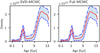 |
Fig. 12 As for Fig. 10 but with higher regularisation. |
| In the text | |
|
Fig. B.1 Influence of the latent dimension q on SVD-MCMC. The top panel shows singular values of the matrix of MILES SSPs. The lower left panel shows the error between filtered credible intervals computed with SVD-MCMC and Full MCMC. The error is measured in the mean Jaccard distance (see equation (B.1)). Beyond q = 15 the error stabilises, signalling converged results. The lower right panel shows the corresponding computation time for SVD-MCMC, where the dashed horizontal line marks the computation time for Full MCMC. In all panels, the vertical dotted line is at q = 15, the value adopted for SVD-MCMC inferences in this work. |
| In the text | |
Current usage metrics show cumulative count of Article Views (full-text article views including HTML views, PDF and ePub downloads, according to the available data) and Abstracts Views on Vision4Press platform.
Data correspond to usage on the plateform after 2015. The current usage metrics is available 48-96 hours after online publication and is updated daily on week days.
Initial download of the metrics may take a while.