| Issue |
A&A
Volume 672, April 2023
|
|
|---|---|---|
| Article Number | A164 | |
| Number of page(s) | 13 | |
| Section | Extragalactic astronomy | |
| DOI | https://doi.org/10.1051/0004-6361/202244560 | |
| Published online | 19 April 2023 | |
Black hole and galaxy co-evolution in radio-loud active galactic nuclei at z ∼ 0.3–4⋆
1
Observatoire de Paris, LERMA, PSL University, Sorbonne Université, CNRS, 75014 Paris, France
e-mail: remi.poitevineau@obspm.fr
2
Dipartimento di Fisica e Astronomia “Augusto Righi”, Alma Mater Studiorum Università di Bologna, Via Gobetti 93/2, 40129 Bologna, Italy
3
INAF – Osservatorio di Astrofisica e Scienza dello Spazio di Bologna, via Gobetti 93/3, 40129 Bologna, Italy
4
Collège de France, 11 Place Marcelin Berthelot, 75231 Paris, France
Received:
21
July
2022
Accepted:
24
January
2023
The relation between the mass of the supermassive black hole (SMBH) in the center of galaxies and their bulge mass or central velocity dispersion is well known. This suggests a coevolution between the SMBHs and their galaxy hosts. Our aim is to study this relation, specifically, for radio loud galaxies, and as a function of redshift z. We selected a sample of 42 radio galaxies and active galactic nuclei (AGN) with broad emission lines and spectroscopic redshifts between z = 0.3 − 4 by cross-matching the low radio frequency sources from Very Large Array (VLA) FIRST with spectroscopically confirmed galaxies from wide-field surveys, including Sloan Digital Sky Survey (SDSS) DR14 ugriz and Dark Energy Survey (DES) DR2 grzY in the optical, Wield Infrared Survey Explorer (WISE), and the Galaxy And Mass Assembly (GAMA) spectroscopic survey. We characterized the stellar mass (M⋆), star formation, and black hole properties (mass of the central SMBH, Eddington ratio η, and jet power, Qjet). The relation between SMBH mass, M⋆, η, and z is placed into context by comparing them with scaling relations (MBH–M⋆, MBH/M⋆–z, MBH–Qjet, and Qjet–η) from the literature. On the basis of a multiwavelength spectral energy distribution modeling, our radio sources are broadly consistent with being on the star-forming main sequence. They have sub-Eddington accretion rates, η ≃ 1% on average, as typically found in type I AGN, while higher accretion rates favor more powerful jets to be launched by the central engine. We find overmassive SMBHs in (17 ± 5)% of our radio sources, similarly to previous studies on nearby early-type galaxies. Altogether, an evolutionary scenario in which radio-mode AGN feedback regulates the accretion onto the SMBHs and the stellar mass assembly of the radio sources is discussed, which may explain the observed phenomenology. This pilot study represents a benchmark for future studies using wide-field surveys such as those with Euclid and the Vera Rubin Observatory.
Key words: quasars: supermassive black holes / Galaxy: evolution / infrared: galaxies / radio continuum: galaxies / Galaxy: nucleus / Galaxy: bulge
Tables A.1 and A.2 are also available at the CDS via anonymous ftp to cdsarc.cds.unistra.fr (130.79.128.5) or via https://cdsarc.cds.unistra.fr/viz-bin/cat/J/A+A/672/A164
© The Authors 2023
 Open Access article, published by EDP Sciences, under the terms of the Creative Commons Attribution License (https://creativecommons.org/licenses/by/4.0), which permits unrestricted use, distribution, and reproduction in any medium, provided the original work is properly cited.
This article is published in open access under the Subscribe to Open model. Subscribe to A&A to support open access publication.
1. Introduction
Supermassive black holes (SMBHs), characterized by masses in the range ∼106 M⊙ to ∼1010 M⊙, are observed to lie at the center of most, if not all, massive galaxies (e.g., Graham 2016). When the central regions of galaxies are sources of radiation because of accretion onto their SMBHs, they are called active galactic nuclei (AGN). AGN are among the strongest proofs for the existence of SMBHs, together with the direct measure of high densities in our Galactic center (e.g., Genzel et al. 2010), and the direct observation of the SMBH shadow at the center of M87 and of the Milky Way itself (The Event Horizon Telescope Collaboration 2019, 2022).
An intrinsic coevolution exists between AGN activity, SMBH growth, galaxy stellar content, and star formation history (e.g., Kormendy & Ho 2013, for a review). In some cases, AGN are jetted and are then called radio-loud AGN. They constitute only 10% of the whole AGN population, but their fraction varies with the stellar mass of the host, from 0 to 30% (Best et al. 2005). Large-scale radio jets are even able to impact the global megaparsec-scale environmental properties via radio-mode AGN feedback, for example, at the center of galaxy (proto-)clusters (e.g., Miley & De Breuck 2008; Fabian 2012; Magliocchetti 2022, for a review).
The mode of SMBH accretion ultimately regulates the excitation properties of radio-loud AGN. It is indeed possible to distinguish two main classes of activity among the radio-loud AGN: high-excitation (HE) and low-excitation (LE) radio galaxies (RG) according to their accretion rate: HERGs typically have accretion rates between 1 and 10% of their Eddington rate, whereas LERGs predominately accrete at a rate below 1% Eddington (Best & Heckman 2012). In HERGs, the material thus progressively loses angular momentum in a geometrically thin disk around the SMBH; this disk is usually optically thick and radiates efficiently. When the accretion rate is below 0.01 the Eddington rate, the AGN is instead characterized by an advection-dominated accretion flow (ADAF; e.g., Narayan & McClintock 2008), which radiates inefficiently. Radio-loud AGN mostly occur in the low-luminosity regime, and ADAFs frequently occur as well.
A major observational breakthrough for the coevolution of galaxies and AGN with their SMBHs was the discovery of a tight correlation in the local universe between the SMBH mass and the mass of their host spheroids (Magorrian et al. 1998; Ferrarese & Merritt 2000). This relation implies a remarkable connection between the assembly of galaxies and the formation and growth of SMBHs at their center (e.g., Heckman & Best 2014, for a review). Models and simulations (Menci et al. 2006; Marulli et al. 2008; Hopkins et al. 2006; Volonteri & Natarajan 2009) have attempted to explain this correlation and its evolution with redshift, as found in several observational studies (e.g., Shields et al. 2006; Sarria et al. 2010; Wang et al. 2010; Merloni et al. 2010; Jahnke et al. 2009; Cisternas et al. 2011; Schramm & Silverman 2013).
There is, however, still a number of related open issues. These include local ellipticals with overmassive SMBHs (Kormendy et al. 1997; van den Bosch et al. 2012; Savorgnan & Graham 2016; Dullo et al. 2021). These overmassive SMBH preferentially occur in galaxy clusters and in brightest cluster galaxies in particular (BCGs; e.g., McConnell & Ma 2013), where environment effects strip the galaxies from their gas and stop star formation and the growth of bulges. Galaxies are then called massive relics and have particularly old stellar population (Trujillo et al. 2014; Martín-Navarro et al. 2015; Ferré-Mateu et al. 2015, 2017). The very discovery of massive SMBHs (MBH ≳ 109 M⊙) in bright quasars at the epoch of reionization (e.g., Bañados et al. 2018; Farina et al. 2022) is a mystery, as it shows that extreme SMBHs can form within 1 Gyr after the Big Bang. The rapid formation of these high-z SMBHs might be explained by invoking some extreme scenarios such as the growth of a 102 − 5 M⊙ seed via super-Eddington accretion (Valiante et al. 2016b; Pezzulli et al. 2017), the direct collapse of an initial gas condensation into a black hole of ∼105 M⊙ (Visbal et al. 2014; Regan et al. 2017), or the merger of massive protogalaxies (e.g., Mayer et al. 2010, 2015; Ferrara et al. 2013; Bonoli et al. 2014).
Altogether, while existing studies show a tight coevolution of SMBHs, AGN, and their host galaxies with cosmic time, this interplay is still substantially debated and unconstrained. This is at least partially due to the difficulty of building large samples of distant AGN with well-characterized stellar and black hole properties.
In order to better understand the growth of SMBHs with cosmic time and their coevolution with their host galaxies, we have built a sample of distant radio-loud AGN spanning about 9 Gyr of cosmic time, between z ∼ 0.3 − 4, with available radio to ultraviolet (UV) spectrophotometric data. Based on this multiwavelength dataset, we assess the properties of the AGN sample, for example, in terms of black hole and stellar masses, jet power, and Eddington ratio. As radio-loud AGN are associated with the most massive black holes and host galaxies (e.g., Best et al. 2005; Chiaberge & Marconi 2011; Shen et al. 2011; Shaw et al. 2012), they are excellent sources in which to investigate the galaxy, AGN, and SMBH coevolution in the high-mass regime.
The paper is organized as follows. In Sect. 2 we describe our sample selection as well as its multiwavelength dataset and properties. In Sect. 3 we report estimates for the black hole, jet, accretion, and stellar properties. In Sect. 4 we describe our comparison sample. The results in terms of the scaling relations of black hole, jet, and host galaxy are reported in Sect. 5. In Sect. 6 we summarize the results and draw our conclusions.
Throughout this work, we adopt a flat ΛCDM cosmology with matter density Ωm = 0.30, dark energy density ΩΛ = 0.70, and Hubble constant h = H0/100 km s−1 Mpc−1 = 0.70.
2. Radio-loud AGN sample
We selected a sample of radio-loud AGN by cross-matching the Very Large Array Faint Images of the Radio Sky at Twenty-centimeters (VLA FIRST) source catalog (Becker et al. 1995) with infrared (IR) to optical spectrophotometric surveys. As further described in the following, the use of IR to UV photometry enables modeling the spectral energy distribution (SED), which ultimately allows us to obtain a good characterization of the galaxy properties, such as the stellar mass (M⋆) and the star formation rate (SFR).
2.1. Dark Energy Survey
We started by considering the Dark Energy Survey (DES The Dark Energy Survey Collaboration 2005, 2016), which is composed of two distinct multiband imaging surveys: a ∼5000 deg2 wide-area grizY survey, and a deep supernova griz survey consisting of six distinct deep fields (Hartley et al. 2021). The coadded source catalog and images from the processing of all six years of DES wide-area survey observations and all five years of DES supernova survey observations have recently been made public with the DES data release 2 (Abbott et al. 2021)1.
To build our sample of distant radio-loud AGN, we limited ourselves to equatorial DES supernova fields that overlapped with the VLA FIRST survey at low radio frequencies. The selection was similar to that of our previous work (Castignani et al. 2019), to which we refer for further details. However, in that study, we focused only on two radio sources, and we investigated their molecular gas content, their cluster environment, as well as the stellar and star formation properties. In this work, we consider instead a more extended sample, as further outlined in the following.
2.2. Radio, optical, and spectroscopic selection
As we are interested in building a sample of extragalactic radio sources, we considered the VLA FIRST survey (Becker et al. 1995), which observed 10 000 deg2 of the North and South Galactic Caps at low radio frequencies (1.4 GHz), down to a point source detection limit of ∼1 mJy. We therefore further limited ourselves to the Stripe 82 area, that is, a 300 deg2 equatorial field that was imaged multiple times by the Sloan Digital Sky Survey (SDSS) and overlaps with the VLA FIRST survey. Similarly, we additionally considered DES supernova deep fields numbered 2, 3, and 5 for our search, as outlined in Sect. 2.1
We cross-matched the low radio frequency VLA FIRST radio source catalog with both the SDSS DR14 ugriz and DES DR1 grizY source catalogs within the considered fields with a search radius of 3 arcsec, consistent with the positional accuracy ∼1 arcsec of FIRST sources. As we are interested in secure distant radio sources, we further restricted ourselves to sources with SDSS DR14 spectroscopic redshifts z > 0.3. The search yielded 158 spectroscopically confirmed radio sources with unique optical counterparts from both SDSS and DES.
2.3. IR selection: WISE
We further searched for IR emission of the radio sources, as found by the W4 filter of the Wide-field Infrared Survey Explorer (WISE; Wright et al. 2010). We therefore cross-correlated our radio sources with the allWISE source catalog2 by adopting a search radius of 6.5 arcsec, consistent with previous work on extragalactic radio sources (e.g., Castignani et al. 2013). The search yielded 154 sources with unique WISE counterparts and W4 magnitudes with a signal-to-noise ratio S/N > 1.
2.4. Broad emission lines from SDSS
As we are interested in assessing black hole masses of the considered radio-loud AGN, we further restricted ourselves to sources with evidence of broad emission lines in the SDSS spectra. To do this, we further selected sources that have Hα, Hβ, Mg II, or C IV emission line fluxes at an S/N > 3, as well as a full width at half maximum FWHM > 1000 km s−1, typical of the broad-line region lines. We used the spZline file3, which contains the results of the emission-line fits for the BOSS spectra of SDSS sources (Bolton et al. 2012). The Gaussian line width σ is reported, and we converted it into the  . This additional spectroscopic selection yielded 21 sources at z ∼ 0.3 − 3.8.
2.5. Radio-loud AGN in GAMA DR3
In addition to the radio-loud AGN selected as described in the previous subsections, we searched for distant radio sources from the third data release (DR) of the Galaxy And Mass Assembly (GAMA) spectroscopic survey. GAMA DR3 (Baldry et al. 2018) provides spectra obtained with the AAOmega multi-object spectrograph on the Anglo-Australian Telescope (AAT) as well as a wealth of ancillary information for more than 200 000 sources.
Similarly to what we did concerning the SDSS spectra, we first selected 632 sources at z > 0.3, with available GAMA DR3 spectra, Hα or Hβ line fluxes at S/N > 3 as well as line widths FWHM > 1000 km s−1, as inferred from single Gaussian modeling4. We selected these sources within the equatorial area of 180 deg2 covered by GAMA DR3 as well as by the 1.4 GHz FIRST VLA survey. For the 632 spectroscopic sources from GAMA, we further limited ourselves to the subsample of 39 galaxies with available 1.4 GHz fluxes from the FIRST VLA survey. Multiple spectra are often available in the GAMA DR3 database. We then inspected each of the available spectra and discarded galaxies with dubious evidence of emission lines, which means that the associated fits are dubious as well. This analysis yielded 21 GAMA DR3 radio sources at z ∼ 0.3 − 0.8. We assigned unique WISE counterparts to them using a 6.5 arcsec search radius, as in Sect. 2.3.
By combining these galaxies, denoted hereafter with the prefix G, with the 21 radio sources with SDSS spectra, denoted with the prefix RS, our final sample comprises 42 sources that we consider hereafter for this study. The main properties of this sample of galaxies are listed in Table A.1.
2.6. Radio and IR properties
We now investigate the low-frequency radio luminosities and the IR colors of our sources. To do this, we first assumed similarly as in previous studies (Condon 1989; Chiaberge et al. 2009; Castignani et al. 2014) a power-law for the radio spectrum, that is, Sν ∝ ν−α, where Sν is the radio flux density at the observer frequency ν, and the spectral index α is fixed to α = 0.8. We then converted the 1.4 GHz VLA radio fluxes S1.4 GHz into rest-frame 1.4 GHz luminosity densities as follows:

where DL is the luminosity distance.
Figure 1 (top) displays our sources in the L1.4 GHz versus redshift plane. They all have L1.4 GHz ≳ 3 × 1030 erg s−1 Hz−1, which is typical of radio-loud AGN, while purely starburst galaxies have lower L1.4 GHz < 1030 erg s−1 Hz−1 (Chiaberge et al. 2009).
 |
Fig. 1. Radio luminosity densities and infrared colors for the radio sources in our sample. Top. 1.4 GHz Radio luminosity density as a function of redshift. Sources are distinguished between AGN (black circles), starbursts (orange triangles), intermediate disks (green squares), and spheroids according to the color-based classification by Stern et al. (2012) and Jarrett et al. (2017). The horizontal line is at Lν = 2 × 1032 erg s−1 Hz−1 and separates low-luminosity radio sources from high-luminosity radio sources. Bottom. WISE color-color plot. Color coding of the data-points is the same as in the top panel. Black dashed lines are overplotted to distinguish the different types of objects (AGN, ULIRGs, spheroids, intermediate disks, starbusts, and LIRGs). |
Furthermore, the majority (71%, i.e., 30/42) of our sources have high radio powers, greater than L1.4 GHz = 2 × 1032 erg s−1 Hz−1, which we used to distinguish between low-luminosity radio sources (LLRS) and high-luminosity radio sources (HLRS), similarly as in previous studies (e.g., Chiaberge et al. 2009; Castignani et al. 2014). As the radio galaxy population has a bimodal distribution in radio power, it is worth mentioning that the adopted LLRS to HLRS luminosity threshold corresponds to the fiducial radio power that fairly separates Faranoff-Riley I (FR I) from FR II radio galaxies (Fanaroff & Riley 1974; Zirbel 1996). Furthermore, as a result of the Malmquist bias associated with the VLA FIRST flux limit of ∼1 mJy, the fraction of HLRSs increases with redshift and reaches unity at z > 1.
Figure 1 (bottom) shows the sources in our sample in the WISE color-color diagram, where sources are distinguished using the color-based classification by Jarrett et al. (2017), as highlighted in the figure. Interestingly, our sample populates only three regions in the diagram. The majority (28 out of 42) of our sources are classified as AGN based on WISE colors. This is expected because they were selected as distant and powerful radio sources at z > 0.3. Based on WISE colors, the remaining sources are fairly equally distributed between the intermediate disk (9 out of 42) and starburst (5 out of 42) classes.
Furthermore, as shown in Fig. 1 (top), the WISE IR colors of the vast majority of z > 1 sources are consistent with AGN contribution. They also show high 1.4 GHz radio luminosities typical of radio-loud quasars (QSOs). The majority (22 out of 42, i.e., 52%) of our sources are in fact classified as quasars in the NASA/IPAC extragalactic database (NED), for instance, with counterparts in the 2dF–SDSS LRG And QSO (2SLAQ; Croom et al. 2009) catalog, or with X-ray conterparts (XMM; Rosen et al. 2016), as outlined in Table A.1.
3. Black hole, jet, accretion, and stellar properties
3.1. Black hole masses
One of the main goals of this work is to investigate the coevolution of central black holes with the host galaxies of the radio-loud AGN in our sample. To do this, we estimated black hole masses using the widely used single-epoch (SE) method, which is particularly suited for distant type 1 AGN. According to this method, black hole masses MBH can be estimated under the assumption that the broad-line region (BLR) is in virial equilibrium, as follows:
where RBLR is the BLR radius, ΔV is the velocity of the BLR clouds that can be estimated from the broad emission line width, f is the virial coefficient that depends on the geometry and kinematics of the BLR, and G is the gravitational constant. The SE method then uses the relation between the BLR size and the AGN optical/UV continuum luminosity empirically found from reverberation mapping (Peterson et al. 2004; Kaspi et al. 2007; Bentz et al. 2009), as well as the tight correlation between the continuum luminosity and that of broad emission lines (e.g., Shen et al. 2011). With these considerations, the black hole mass can be expressed as

where the coefficients a, b, and c are empirically calibrated against local AGNs with reverberation mapping masses or using different lines. L and FWHM are the line luminosity and width. We used the coefficients obtained for the Hα, Hβ, Mg II, and C IV broad emission lines by Shen et al. (2011) and Shaw et al. (2012). These are widely used lines that are redshifted in the optical domain, depending on the redshift of the source. These lines indeed enable estimates of black hole masses over a wide range of redhifts. Similarly to previous studies (Shaw et al. 2012; Castignani et al. 2013), we used Hα, Hβ, and Mg II for sources at z < 1 and the Mg II and C IV lines for sources at higher redshifts. When multiple broad emission lines were available for a given sources, we adopted the following order of preference: Hα, Hβ, Mg II, and C IV (see, e.g., Shen & Liu 2012 for more details). In Table 1 we report the coefficients used in this work, and in Table A.2 we list the black hole masses.
3.2. Jet power
The sources in our sample are radio-loud AGN that are typically characterized by jetted outflows that strongly emit at radio wavelengths mainly via synchrotron emission. By studying jet properties such as its total power, we investigate the complex interplay between the jet, the black hole, and the gas accretion onto it, which is commonly referred to as radio-mode AGN feedback (e.g., Fabian 2012, for a review). Following previous work by Willott et al. (1999), we estimate the jet power as
where L151 MHz is the extended total radio luminosity density at 151 MHz in the rest frame, and ξ ranges between 10 and 20. We used an intermediate value ξ = 15. To estimate L151 MHz, we extrapolated the L1.4 GHz luminosity densities assuming an isotropic emission and a power law with α = 0.8, as further described in Sect. 2.6. The resulting jet powers are reported in Table A.2.
3.3. Eddington ratio
We wish to link the gas accretion onto the black hole with the AGN properties. We therefore estimated the Eddington ratio, which is defined as

where Ldisk and LEdd are the disk and Eddington luminosities. The latter can be expressed as
To estimate the disk luminosity, we instead followed the prescriptions described in Celotti et al. (1997). First, we assumed that BLR contributes ∼10% of the total disk luminosity, that is, Ldisk ≃ 10 LBLR. To estimate the BLR luminosity, we then used the line ratios reported in Francis et al. (1991), which are typical line luminosities of bright QSOs, normalized to that of the Lyα emission. The BLR luminosity can therefore be estimated as
where Li, obs is the luminosity of the observed ith line in the BLR, and  is the line ratio of the ith line presented in the table of Francis et al. (1991). With these prescriptions, the total normalized BLR luminosity is equal to
  , where
  was fixed as a reference.
The resulting Eddington ratios are reported in Table A.2. They are mostly in the range log η ∼ ( − 4; −1), with a median = −1.9, as typically found for type 1 radio-loud AGN, but lower than the ratios of type 2 quasars (e.g., Castignani et al. 2013; Kong & Ho 2018).
3.4. SED modeling
The radio sources in our sample have a broad multiwavelength photometric coverage from the UV to the IR, which enables the determination of stellar masses and SFR estimates via SED modeling.
For the GAMA sources in our sample, we considered the SED fits by Driver et al. (2018) performed with MAGPHYS (da Cunha et al. 2008). Photometric data include GALEX (Martin et al. 2005; Morrissey et al. 2007) in the UV, SDSS (York et al. 2000) in the optical, as well as the VISTA Kilo-degree IR Galaxy Survey (VIKING, Edge et al. 2013), WISE (Wright et al. 2010), and Herschel- ATLAS (Eales et al. 2010; Valiante et al. 2016a) in the near- to far-IR.
For the sources in the DES SN deep fields, available photometry includes GALEX in the UV, ugriz (SDSS) and grizY (DES) magnitudes in the optical, WISE data in the near-IR, as well as IRAS upper limits in the far-IR, which we gathered as in Castignani et al. (2019), to which we refer for further details. In this previous work, we followed up two radio sources in molecular gas in dense megaparsec-scale environments at z = 0.4 and z = 0.6 within the DES SN deep fields, while we enlarge the sample here to investigate the coevolution of black holes with radio sources.
Analogously to Castignani et al. (2019), we then performed fits to the SEDs using LePhare (Arnouts et al. 1999; Ilbert et al. 2006). Following the prescriptions provided for the LePhare code, we fit the far-IR data separately to account for possible dust emission, using the Chary & Elbaz (2001) library consisting of 105 templates. The remaining photometric data points at shorter wavelengths were fit using the CE_NEW_MOD library, which consists of 66 galaxy templates based on linear interpolation of the four original SEDs of Coleman et al. (1980). We then converted the rest frame (8.0–1000) μm IR (dust) luminosity into an SFR estimate by using the Kennicutt (1998) relation, calibrated to a Chabrier (2003) initial mass function. The SEDs of four of our radio sources are shown in Fig. 2. RS 81 and 83 have prominent elliptical emission in the optical domain, while their IR emission is consistent with dust emission due to star formation. They are indeed classified as intermediate disks based on WISE colors. RS 113 and 237 are WISE AGN and show steep SEDs at near-IR to optical wavelengths, which suggests that the emission is contaminated by nonthermal AGN emission.
 |
Fig. 2. Examples of SEDs of the radio sources in our sample with black hole mass estimates. The IDs, names, and redshifts of the galaxies are shown at the top left of each panel. Data-points are from GALEX (brown dots), SDSS (red pentagons), DES (blue squares), WISE (green triangles), and IRAS (yellow upper limits). Dashed and solid lines are the best-fit models for the stellar and dust components, respectively. |
3.5. SFR versus stellar mass
Figure 3 displays the radio sources of our sample in the SFR versus stellar mass (M⋆) plane resulting from the SED fits. The sources are color-coded according to the redshift, while the different symbols correspond to the WISE classification.
 |
Fig. 3. SFR vs. stellar mass for the galaxies in our sample. Sources are color-coded according to their redshift, while the different symbols correspond to the different WISE classes (AGN as circles, starbursts as triangles, and intermediate disks as squares), as in Fig. 1. Upper limits to the SFRs are indicated with arrows. The diagonal lines correspond to the MS model prescriptions by Speagle et al. (2014) at z = 0.2, 1, and 2. The red cross in the bottom right corner shows the typical uncertainties of ∼0.3 dex for both SFRs and stellar masses. |
Overall, the sources are massive, with log(M⋆/M⊙)≃10.3 − 12.0 (median = 10.1), which agrees with them being radio-loud AGN, which are indeed typically hosted by massive ellipticals (Best et al. 2005). Our galaxies also mostly lie along the star-forming main sequence (MS), although with a large scatter. The mean specific SFR is sSFR = 0.40 ± 0.44 Gyr−1, where the root mean square (rms) dispersion is reported as uncertainty.
Galaxies at higher redshifts tend to have higher SFRs, in agreement with the MS model prescriptions (Speagle et al. 2014). However, as highlighted in Sect. 2.6, the fraction of sources with AGN contamination also increases with redshift, which may result in biased-high SFRs. The latter may be the case where the optical-IR SED is steep, and thus the IR emission is likely dominated by the AGN contribution, more than star formation. To overcome this limitation, we conservatively reconsidered the SFR estimates and assigned upper limits when the SFRs largely exceeded 100 M⋆/yr or in the cases of steep-spectrum SEDs (e.g., for RS 113 and 237 mentioned above). Namely, we considered as steep spectra those AGN whose optical-IR SED has a characteristic power-law behavior Fλ ∝ λ−1. We verified a posteriori that these radio sources are indeed mostly located in the upper part of the MS and are classified as WISE AGN.
4. Comparison sample
To place the AGN in our sample into context, we additionally considered a compilation of sources with available black hole and stellar mass estimates. We first took the 30 nearby galaxies from Häring & Rix (2004). Galaxy masses were derived by the authors through Jeans equation modeling or were adopted from dynamical models in the literature, and black hole masses are from Tremaine et al. (2002) and references therein. Then, we added the 35 nearby galaxies from the sample of McConnell & Ma (2013), who expanded and revised available galaxy bulge masses and dynamical measurements of black hole masses. Cisternas et al. (2011) has 32 type 1 AGN at z = 0.3 − 0.9, drawn from the XMM-COSMOS survey. Available stellar masses are based on the modeling of HST images, taking both AGN and host galaxy contributions into account, and black hole masses are from Hβ (Trump et al. 2009). We also added the 18 broad-line X-ray AGN 0.5 < z < 1.2 in the Extended Chandra Deep Field-South Survey from Schramm & Silverman (2013), who estimated Mg II-based black hole masses, as well as HST color-based stellar mass estimates. We included 78 radio-quite type 1 AGN at z ≃ 1 − 2 in the COSMOS survey (Merloni et al. 2010). Stellar masses were determined via SED fitting, and black hole masses are based on the Mg II emission lines of VIMOS/VLT spectra. The 10 type 1 AGN at 1 < z < 2 reported in COSMOS from Jahnke et al. (2009), who estimated HST color- based stellar masses, and the virial black hole masses come from the spectroscopic COSMOS Magellan/IMACS and zCOSMOS surveys. We added the 53 radio-quiet QSOs at z < 3 from Decarli et al. (2010a,b). Virial black hole masses come from the Hβ, Mg II, and C IV emission lines, and the stellar masses were estimated by the authors assuming a stellar R-band mass-to-light ratio. Targett et al. (2012) gives us the information about 2 SDSS luminous quasars at z ∼ 4. Virial black hole mass estimates come from C IV emission, and the stellar masses were estimated on the basis of the evolutionary synthesis models of Bruzual & Charlot (2003). Shields et al. (2006) reported 9 distant z ∼ 1.4 − 6.4 QSOs. Black hole masses were derived from broad emission lines, and they used CO emission line widths to infer the dynamical bulge masses. Finally, we added the 7 QSOs at z ≃ 6 from Wang et al. (2010). They calculated the stellar mass as the difference between the bulge dynamical mass and the CO molecular gas mass. For these QSOs, we used the black hole masses adopted by the authors that were estimated using the AGN continuum luminosity (Jiang et al. 2006; Wang et al. 2008).
In addition to the sources listed above, the second group of galaxies that we used as a comparison is composed by powerful AGN with available estimates of the black hole mass, jet power, and Eddington ratio. We added the 44 radio-loud AGN studied in Le et al. (2018) at redshifts z < 0.2, which is lower than those of the radio sources in our sample. These sources have estimates of the jet powers (Le et al. 2018) and of their black hole masses (Allen et al. 2006; Balmaverde et al. 2008). We also added the 208 γ-ray Fermi blazars at 0 < z < 3.1 from Xiong & Zhang (2014). Virial black hole mass estimates mostly come from different broad emission lines, and the rest were obtained from scaling relations. Jet powers Qjet are mostly from Nemmen et al. (2012) and were estimated using the correlation between the extended radio emission and the jet power. Alternatively, Xiong & Zhang (2014) calculated Qjet using the scaling relation provided by Nemmen et al. (2012) between the γ-ray luminosity and the kinetic power. Finally, Liu et al. (2006) has 146 radio-loud QSOs at 0.1 < z < 2.5, classified as flat-spectrum (54%) or steep-spectrum radio quasars (46%). The black hole virial masses come from the Hβ, Mg II, or C IV emission lines. The jet power were calculated by the authors using low-frequency radio emission, following Punsly (2005).
These sources outlined above are radio-loud AGN. However, we verified that none of them are included in our sample. While these studies investigated the black hole and jet properties of large samples of radio sources, they did not characterize their IR to optical SEDs, as we did here for our smaller sample of radio sources.
5. Results
In this section, we report different scaling relations for the radio sources in our sample, including black hole and stellar masses, jet powers, Eddington ratios, and the redshifts. We also include the sources from the literature as outlined in Sect. 4 as a comparison, as well as the scaling relations derived in previous studies.
5.1. Black hole versus stellar mass relation
We start by considering black hole and stellar masses and their relative evolution with redshift. Figure 4 displays the black hole mass (MBH) versus the stellar mass (M⋆). Interestingly, our radio-loud sources nicely follow the trend previously observed for different samples of both local galaxies and distant AGN, overplotted in the figure, and for those inferred by the scaling relations, which were also reported (Sani et al. 2011; Häring & Rix 2004; DeGraf et al. 2015).
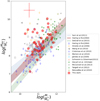 |
Fig. 4. Scatter plot of black hole vs. stellar mass. Filled red dots correspond to our sample of radio sources, and the sources in the comparison sample are shown as open symbols. Scaling relations are overlaid (Sani et al. 2011; DeGraf et al. 2015; Häring & Rix 2004). The legend at the right displays the adopted color code. The red cross in the top left corner shows the typical uncertainties ∼0.4 dex and ∼0.3 dex for the black hole and stellar masses, respectively. |
In particular, our sources populate the high log(MBH/M⊙)≃7.1 − 10.0 and high log(M⋆/M⊙)≃10.2 − 12.0 region in Fig. 4 densely, which agrees with the fact that radio-loud AGN are almost invariably associated with the most massive galaxies and black holes. Interestingly, a substantial fraction of our sources 9/42 (i.e., 21%) have black hole masses log(MBH/M⊙) > 9 well above the scaling relations for both local (Häring & Rix 2004; Sani et al. 2011) and distant sources at the median redshift z = 0.6 of our sample (DeGraf et al. 2015). This behavior suggests that the growth of black hole masses in radio-loud AGN largely occurs at early z > 1 epochs, while the early stellar mass assembly may not be equally effective. Substantial growth of the stellar mass may take place even at lower redshifts in order to flatten the observed MBH-M⋆ scaling relation by z = 0. Previous studies indeed suggested that massive ellipticals may double their stellar mass between z = 1 and z = 0 (Ilbert et al. 2010; Lidman et al. 2012).
We further investigate this evolutionary scenario in Fig. 5, which shows the MBH/M⋆ ratio as a function of redshift. The large majority (36 out of 42, i.e., 86%) of our radio sources have MBH/M⋆ ratios that are similar to those of AGN in the comparison sample at similar redshifts, and they agree with model prescriptions by McLure et al. (2006), which are overplotted as dashed lines in Fig. 5.
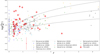 |
Fig. 5. Black hole to stellar mass ratio as a function of redshift for our sample of radio sources (filled red dots) and for the galaxies in our comparison sample (open symbols). The dashed black lines correspond to the evolutionary model described by McLure et al. (2006), along with the associated 1σ uncertainty. The color-coding is reported in the legend in the bottom right corner. The error bars to the left of the legend show the typical ∼0.5 dex uncertainty in log(MBH/M⋆). |
It is worth mentioning that our sample of radio sources is flux limited. However, we expect the Malmquist bias to have a marginal impact on the (MBH/M⋆) ratio. MBH and M⋆ both scale with the BLR line and the IR to optical luminosities, respectively, and therefore have a similar dependence on redshift via the luminosity distance. Furthermore, as shown in Fig. 5, at fixed redshift, the MBH/M⋆ ratios of both our radio sources and those in the comparison sample span a broad range. Similarly, when plotting M⋆ and MBH against redshift separately, we did not find any clear trend, as indeed the points are scattered at fixed redshift. These findings suggest that any possible Malmquist bias likely has a subdominant effect.
There are, however, five clear outliers among our radio sources. RS 197 at the highest redshift z = 3.79 has a low log(MBH/M⋆) = − 3.2, which is well below the expected range of values, according to the McLure et al. (2006) model prescription. Furthermore, a substantial fraction (five sources, i.e., 12%) of our radio loud AGN, namely RS 214, RS 237, G 537618, G 721940, and G 746605, at redshifts between z ∼ 0.37 − 0.95, have high log MBH/M⋆ ratios in the range ∼(−1.69; −1.0), which is well above the model predictions displayed in Fig. 5, as well as higher than the ratios found in AGN at similar redshifts. Indeed, in the redshift range z ∼ 0.3 − 3.8 spanned by our radio sources, there are only 3 out of 186 (i.e., 1.6%) AGN with log MBH/M⋆ > −1.69 in our comparison sample, while the proportion is significantly higher (12%) for our radio-loud AGN. These results suggest that a non-negligible fraction of radio-loud AGN may experience a different stellar mass assembly path than radio-quiet AGN. We stress that these five radio sources are a subsample of the nine outliers of Fig. 4, as discussed above, and have high S/N line fluxes in Hβ or Mg II, which yielded robust MBH estimates. The only exception is represented by G 721940, for which the Hβ emission and associated FWHM are at lower S/N ∼ 2, as highlighted in Table A.2.
The excess of overmassive SMBHs in radio-loud AGN suggests that their stellar and SMBH mass buildup is regulated by their large-scale radio jets. A possible scenario is that SMBHs of the subpopulation with high MBH/M⋆ are mature, that is, their mass has been effectively assembled already by redshift z = 1 via accretion (e.g., Delvecchio et al. 2018). On the other hand, their stellar mass growth may not have occurred as effectively as in the overall AGN population, plausibly because of radio-mode AGN feedback (Fabian 2012). While the accretion of hot gas onto the SMBH sustains the AGN activity and the SMBH growth, the large scale radio jets may prevent accretion and cooling of the inter-galactic medium gas, which is ultimately responsible for the stellar mass assembly. Altogether, we suggest that radio-mode AGN feedback results in the observed high values for MBH/M⋆ in radio-loud AGN.
In order to investigate further this scenario, we link accretion and jet properties to the black hole mass in the next sections by considering both the jet power and Eddington ratio of our radio sources. We stress that the usual MBH − Mbulge or MBH − σ relations typically refer to the central spheroid and not to the total stellar mass (e.g., Kormendy & Ho 2013). However, our radio-loud AGN sample is composed in a large majority of early-type galaxies, where the spheroid constitutes most of the stellar mass, and this approximation is justified. Furthermore, because of the potential AGN contamination to the SED, the stellar mass may be biased high. This implies that MBH/M⋆ ratios can be even higher than reported. By considering MBH/M⋆ ratios as lower limits, we would have an even stronger discrepancy, in particular, for the subsample of high MBH/M⋆ radio sources mentioned above, with respect to the model prescriptions and the comparison sample of distant AGN at fixed resdshift. All these results seem to corroborate the scenario that SMBH growth is more rapid than stellar mass assembly, and this is particularly true for distant radio sources, in comparison to the overall AGN population.
5.2. Jet power, black hole mass, and accretion
As mentioned in the previous sections, mechanical radio-mode AGN feedback can regulate the cooling of hot gas in the intergalactic medium, and thus the stellar mass growth of the host galaxy itself as well as the accretion onto the central SMBH. To better understand the interplay between jet, black hole, and accretion properties, in Fig. 6 we show the jet power Qjet (see Sect. 3.2), plotted against the black hole mass MBH. The radio sources of our sample are highlighted, and we also overplot the comparison sources outlined in Sect. 4 (Liu et al. 2006; Balmaverde et al. 2008; Xiong & Zhang 2014; Chen et al. 2015).
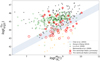 |
Fig. 6. Jet power vs. black hole mass. The diagonal dashed region represents the model reported in previous studies (Wu & Cao 2008; Chen et al. 2015) that distinguishes between FR I and FR II radio galaxies. Sources from our sample are distinguished between high- and low-luminosity radio sources. Sources from our comparison sample are also shown. We refer to the legend for the color-code. |
Our radio-loud AGN densely populate the upper right region of the Qjet-MBH plane, which is occupied by sources with high values of both the black hole mass (MBH ≳ 108 M⊙) and the jet power (Qjet ≳ 1043 erg s−1). Sources in the comparison sample similarly occupy this region, while they also extend to lower values of MBH (Liu et al. 2006; Xiong & Zhang 2014) and jet power (Balmaverde et al. 2008). These results suggest that the distant radio-loud AGN, quite independently of the redshift, are almost invariably associated with massive black holes and powerful radio jets. This agrees with the tight connection existing between black hole accretion and jet production in powerful radio-loud AGN (e.g., Ghisellini et al. 2014; Sbarrato et al. 2014; Inoue et al. 2017).
Furthermore, HLRSs are characterized by a jet power that is typically higher than in LLRSs. As discussed in Sect. 2.6, these two classes indeed have 1.4 GHz rest-frame luminosity densities typical of FR II and FR I radio galaxies, respectively. As Qjet increases with the radio luminosity density (Eq. (4)), high-luminosity radio sources have higher Qjet values than low-luminosity sources. Furthermore, the two classes of LLRGs and HLRGs are also delimited in the Qjet-MBH plane by the relation found in previous studies (Wu & Cao 2008; Chen et al. 2015), originally used to distinguish between FR I and FR II radio galaxy populations. The clear separation of LLRGs and HLRGs in the Qjet versus MBH plane can be explained by combining the MBH versus Mbulge relation for elliptical galaxies and the relation between Qjet and the host galaxy optical luminosity (Ledlow & Owen 1996) that separates the FR I and FR II radio galaxies. The combination of these two relations also implies the observed spread of our sources in Fig. 6. We did not find any significant correlation (as measured with the Spearman test) between Qjet and MBH for our radio sources.
Figure 7 displays instead the jet power, plotted against the Eddington ratio η (see Sect. 3.3) for our radio sources and the galaxies in the comparison sample (Xiong & Zhang 2014; Liu et al. 2006). Higher accretion rates favor more powerful jets to be launched by the central engine, as indeed the jet power increases with increasing Eddington ratio. For our sample of radio sources, we find that the two quantities are well correlated at a level of 2.9-σ (p-value = 3.30 × 10⁻³) by means of the Spearman test. No clear distinction in terms of η is found between the two classes of low- and high-luminosity radio sources, which are distinguished in Fig. 7. However, as pointed out in Sect. 3.3 our radio sources have an Eddington ratio of log η = −1.9 on average. This value is typical of radiatively efficient accretion disks, such as the Shakura & Sunyaev (1973) optically thick and geometrically thin accretion disk, which is commonly invoked to explain the optical-UV emission in type I AGN (e.g., Ghisellini et al. 2010; Castignani et al. 2013).
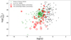 |
Fig. 7. Jet power vs. the Eddington ratio (η) of the associated black hole. In addition to our sample, the data found in Xiong & Zhang (2014) and Liu et al. (2006) are plotted. |
We can then estimate the accretion rate Ṁ =Ldisk/(ϵ c2), where ϵ is the mass-to-light conversion efficiency, for which we adopted the standard value ϵ = 0.1, which is typical of radiatively efficient disks. For our radio sources, we obtain a median (mean) accretion rate of 0.16 M⊙ yr−1 (0.6 M⊙ yr−1), which corresponds to a substantial SMBH mass growth of ΔMBH = 1.6 × 10⁶ M⊙ (6.0 × 10⁶ M⊙) over an AGN duty cycle with typical duration of ∼107 yr.
Altogether, the fact that the SMBHs of the radio sources in our sample accrete at a sub-Edddington rate, regardless of their redshift, suggests that most of their mass has likely been built up at earlier epochs. Furthermore, while on one hand, the observed accretion state sustains both the nuclear activity and the SMBH growth at subparsec scales, on the other hand, it also ultimately favors the persistence of large-scale radio jets, which may prevent the host galaxy from accreting gas at kiloparsec scales and thus form stars effectively. This radio-mode AGN feedback may be responsible for the presence of overmassive SMBHs in our sample of radio-loud AGN. It is worth mentioning that the five z ∼ 0.37 − 0.95 radio sources with high MBH/M⋆ ratios that we discussed in Sect. 5.1 accrete a sub-Eddington rate of η ∼ 1%, while they have a normal jet power Qjet ∼ 1044 erg s−1 on average.
5.3. Radio-loud AGN and their environments
A substantial fraction (17 ± 5)% of our radio sources have high MBH/M⋆ ratios (Sect. 5.1) and may be early-type galaxies at the center of clusters. For these galaxies, the stellar mass assembly may have been halted, with reduced star formation activity, as typically found in cluster core ellipticals, while their black holes continue to grow via accretion. This interpretation is consistent with earlier studies (e.g., Trujillo et al. 2014) as well as with the substantial fraction (19%) of radio sources in our sample with low SFR < 5 M⊙/yr, while many others have SFR upper limits. It is indeed known that cluster-core early-type galaxies tend to be outliers in the MBH vs. Mbulge relation (e.g., McConnell & Ma 2013). A famous example of a possibly overmassive black hole is the case of NGC 1277, which is a lenticular galaxy in the Perseus cluster (e.g., van den Bosch et al. 2012; Emsellem 2013; Scharwächter et al. 2016).
Motivated by these studies, we searched in the literature for clusters around the radio sources in our sample, searching by coordinates in the NASA/IPAC Extragalactic Database (NED). NED includes several catalogs of clusters that were identified in wide-field surveys (Goto et al. 2002; Koester et al. 2007; McConnachie et al. 2009; Hao et al. 2010; Durret et al. 2011, 2015; Wen et al. 2012; Radovich et al. 2017; Rykoff et al. 2012; Oguri et al. 2018). Our search yielded three matches. Radio sources RS 49, G 372455, and G 748815 are in the cores (at cluster-centric distances ≲0.5 Mpc) of the clusters [LIK2015] J034.16359-04.73395 (z = 0.89; Lee et al. 2015), WHL J090325.6+011215 (z = 0.31; Wen et al. 2012; Wen & Han 2015), and HSCS J142538+002320 (z = 0.33; Oguri et al. 2018), respectively. These clusters have redshifts that are consistent with those of the radio sources as well as richness-based masses M200 ∼ (0.9 − 3.0)×1014 M⊙. These are therefore moderately massive clusters at intermediate to high redshifts. The three associated radio sources instead have moderately overmassive black holes log(MBH/M⊙)≃8.6 − 9.3, in particular, in comparison to the stellar masses of the systems −2.65 ≲ log(MBH/M⋆)≲ − 2.24 (see Fig. 5).
These results support the interpretation described above that the cluster environments tend to prevent the stellar mass assembly of cluster early-type galaxies, resulting in observed overmassive black holes. Nevertheless, it is worth mentioning that only three radio sources of our sample are found in clusters. However, this is expected as clusters at higher redshifts (z ≳ 1) or with lower masses M200 ≲ 1 × 10¹⁴ M⊙ typical of rich groups are more difficult to find with current surveys and observational facilities. It is therefore possible that additional galaxies are hosted in clusters, as distant radio sources are often found in dense megaparsec-scale environments (e.g., Galametz et al. 2012; Castignani et al. 2014; Malavasi et al. 2015; Golden-Marx et al. 2019; Moravec et al. 2020).
6. Discussion and conclusions
We have investigated the evolution of distant radio-loud AGN, as well their coevolution with their host galaxies and the SMBHs at their center. To do this, we built a sample of 42 radio-loud AGN with spectroscopic redshifts between z ∼ 0.3 − 3.8 by cross-matching the 1.4 GHz VLA FIRST point-source catalog with available IR to optical spectrophotometric surveys including SDSS and DES in the optical, WISE in the IR, and the Galaxy And Mass Assembly (GAMA) spectroscopic survey. As we are interested in assessing the SMBH masses, the 42 galaxies were further selected by requiring broad emission lines in Hα, Hβ, Mg II, or C IV, with an FWHM > 1000 km s−1. Based on the available multiwavelength photometry, we modeled the SEDs of the sources in the sample, and then derived estimates of the stellar mass (M⋆) and SFR for all sources, while for GAMA sources, we took them from the literature. We find that the 42 radio sources are broadly consistent with the star-forming main sequence.
For all sources, we then estimated i) the black hole mass MBH, based on single-epoch broad-line region spectra, ii) the ratio of black hole to stellar mass, MBH/M⋆, iii) the jet power Qjet, on the basis of the low-frequency radio continuum emission, and iv) the Eddington ratio η. Although samples of distant AGN with SMBH mass estimates are rapidly growing (e.g., Shen et al. 2011; Shaw et al. 2012; Dabhade et al. 2020; Rakshit et al. 2020; Gloudemans et al. 2021; Li et al. 2022), our study still represents one of the first in which all these quantities are derived simultaneously for a single sample of distant radio-loud AGN.
Our radio sources have log(MBH/M⊙) ≃ 7.1 − 10.0 and high log(M⋆/M⊙) ≃ 10.2 − 12.0, which agrees with the fact that radio-loud AGN are almost invariably associated with the most massive galaxies and black holes (e.g., Best et al. 2005; Chiaberge & Marconi 2011). While overall our sources follow the expected trends previously found in the literature, a substantial fraction of our sources, 9 out of 42 (i.e., 21%), have black hole masses log(MBH/M⊙) > 9 well above the values predicted by the scaling relations (Häring & Rix 2004; Sani et al. 2011; DeGraf et al. 2015). In particular, five sources out of the nine (12% of the full radio source sample) are clearly overmassive outliers, with MBH/M⋆ > 2%. This fraction is remarkably higher than that of 1.6% found for AGN at similar redshifts from the literature. These overmassive SMBHs are thus the high-z counterparts of overmassive SMBHs found in previous studies of nearby early-type galaxies (e.g., McConnell & Ma 2013; Trujillo et al. 2014).
Our results imply that the growth of black hole masses in at least a substantial fraction of radio-loud AGN largely occurs at early epochs, while the early stellar mass assembly may not be so efficient. This population of radio-loud AGN with high MBH/M⋆ ratios have likely experienced a different stellar mass growth than other types of AGN, and we further investigated this scenario in terms of additional complementary probes.
Following early studies on nearby galaxies (e.g., McConnell & Ma 2013; Trujillo et al. 2014), we found that three of our radio-loud AGN with moderately overmassive SMBHs are hosted in clusters from the literature, while clusters and groups around the majority of the remaining radio-loud AGN will likely be detected with forthcoming surveys such as Euclid (Euclid Collaboration 2019). These results suggest that the cluster environments tend to prevent the stellar mass assembly of cluster early-type galaxies, possibly via radio-mode AGN feedback.
We found that the nuclear accretion and jet properties of the SMBHs of the radio sources in our sample accrete at a sub-Eddington rate (η ∼ 1%) on average, where higher accretion rates favor more powerful jets to be launched by the central engine. We also find that high jet powers (Qjet ≳ 1045 erg s−1) are invariably associated with high radio luminosity sources (L1.4 GHz > 2 × 1032 erg s−1 Hz−1). Altogether, the observed accretion state sustains both the nuclear activity and the SMBH growth at subparsec scales, while it ultimately favors the persistence of large-scale radio jets, which may prevent the host galaxy from accreting gas at kiloparsec scales and thus form stars effectively. Radio-mode AGN feedback may be responsible for the presence of overmassive SMBHs in our sample of radio-loud AGN.
Targeted observations of the ionized and the molecular gas are nevertheless needed to further investigate the proposed radio-mode AGN feedback scenario. Future studies on larger and higher-redshift samples of radio-loud AGN will become possible with the advent of forthcoming radio to optical surveys such as those with the Vera Rubin Observatory and Euclid in the IR-optical, SKA in radio, and its pathfinders and precursors (LOFAR, ASKAP, and MeerKAT).
Acknowledgments
We thank the anonymous referee for helpful comments which contributed to improve the paper. GC acknowledges the support from the grants ASI n.2018-23-HH.0 and PRIN-MIUR 2017 WSCC32. We thank Christophe Benoist for helpful discussion about the exploitation of DES data. This publication makes use of data products from the Wide-field Infrared Survey Explorer, which is a joint project of the University of California, Los Angeles, and the Jet Propulsion Laboratory/California Institute of Technology, and NEOWISE, which is a project of the Jet Propulsion Laboratory/California Institute of Technology. WISE and NEOWISE are funded by the National Aeronautics and Space Administration. This research has made use of the NASA/IPAC Extragalactic Database (NED), which is operated by the Jet Propulsion Laboratory, California Institute of Technology, under contract with the National Aeronautics and Space Administration. This project used public archival data from the Dark Energy Survey (DES). Funding for the DES Projects has been provided by the U.S. Department of Energy, the U.S. National Science Foundation, the Ministry of Science and Education of Spain, the Science and Technology FacilitiesCouncil of the United Kingdom, the Higher Education Funding Council for England, the National Center for Supercomputing Applications at the University of Illinois at Urbana-Champaign, the Kavli Institute of Cosmological Physics at the University of Chicago, the Center for Cosmology and Astro-Particle Physics at the Ohio State University, the Mitchell Institute for Fundamental Physics and Astronomy at Texas A&M University, Financiadora de Estudos e Projetos, Fundação Carlos Chagas Filho de Amparo à Pesquisa do Estado do Rio de Janeiro, Conselho Nacional de Desenvolvimento Científico e Tecnológico and the Ministério da Ciência, Tecnologia e Inovação, the Deutsche Forschungsgemeinschaft, and the Collaborating Institutions in the Dark Energy Survey. The Collaborating Institutions are Argonne National Laboratory, the University of California at Santa Cruz, the University of Cambridge, Centro de Investigaciones Energéticas, Medioambientales y Tecnológicas-Madrid, the University of Chicago, University College London, the DES-Brazil Consortium, the University of Edinburgh, the Eidgenössische Technische Hochschule (ETH) Zürich, Fermi National Accelerator Laboratory, the University of Illinois at Urbana-Champaign, the Institut de Ciències de l’Espai (IEEC/CSIC), the Institut de Física d’Altes Energies, Lawrence Berkeley National Laboratory, the Ludwig-Maximilians Universität München and the associated Excellence Cluster Universe, the University of Michigan, the National Optical Astronomy Observatory, the University of Nottingham, The Ohio State University, the OzDES Membership Consortium, the University of Pennsylvania, the University of Portsmouth, SLAC National Accelerator Laboratory, Stanford University, the University of Sussex, and Texas A&M University. Based in part on observations at Cerro Tololo Inter-American Observatory, National Optical Astronomy Observatory, which is operated by the Association of Universities for Research in Astronomy (AURA) under a cooperative agreement with the National Science Foundation.
References
- Abbott, T. M. C., Adamów, M., Aguena, M., et al. 2021, ApJS, 255, 20 [NASA ADS] [CrossRef] [Google Scholar]
- Allen, S. W., Dunn, R. J. H., Fabian, A. C., Taylor, G. B., & Reynolds, C. S. 2006, MNRAS, 372, 21 [NASA ADS] [CrossRef] [Google Scholar]
- Arnouts, S., Cristiani, S., Moscardini, L., et al. 1999, MNRAS, 310, 540 [Google Scholar]
- Baldry, I. K., Liske, J., Brown, M. J. I., et al. 2018, MNRAS, 474, 3875 [Google Scholar]
- Balmaverde, B., Baldi, R. D., & Capetti, A. 2008, A&A, 486, 119 [NASA ADS] [CrossRef] [EDP Sciences] [Google Scholar]
- Bañados, E., Venemans, B. P., Mazzucchelli, C., et al. 2018, Nature, 553, 473 [Google Scholar]
- Becker, R. H., White, R. L., & Helfand, D. J. 1995, ApJ, 450, 559 [Google Scholar]
- Bentz, M. C., Walsh, J. L., Barth, A. J., et al. 2009, ApJ, 705, 199 [NASA ADS] [CrossRef] [Google Scholar]
- Best, P. N., & Heckman, T. M. 2012, MNRAS, 421, 1569 [NASA ADS] [CrossRef] [Google Scholar]
- Best, P. N., Kauffmann, G., Heckman, T. M., et al. 2005, MNRAS, 362, 25 [Google Scholar]
- Bolton, A. S., Schlegel, D. J., Aubourg, É., et al. 2012, AJ, 144, 144 [NASA ADS] [CrossRef] [Google Scholar]
- Bonoli, S., Mayer, L., & Callegari, S. 2014, MNRAS, 437, 1576 [NASA ADS] [CrossRef] [Google Scholar]
- Bruzual, G., & Charlot, S. 2003, MNRAS, 344, 1000 [NASA ADS] [CrossRef] [Google Scholar]
- Castignani, G., Haardt, F., Lapi, A., et al. 2013, A&A, 560, A28 [NASA ADS] [CrossRef] [EDP Sciences] [Google Scholar]
- Castignani, G., Chiaberge, M., Celotti, A., Norman, C., & De Zotti, G. 2014, ApJ, 792, 114 [NASA ADS] [CrossRef] [Google Scholar]
- Castignani, G., Combes, F., Salomé, P., et al. 2019, A&A, 623, A48 [NASA ADS] [CrossRef] [EDP Sciences] [Google Scholar]
- Celotti, A., Padovani, P., & Ghisellini, G. 1997, MNRAS, 286, 415 [NASA ADS] [CrossRef] [Google Scholar]
- Chabrier, G. 2003, PASP, 115, 763 [Google Scholar]
- Chary, R., & Elbaz, D. 2001, ApJ, 556, 562 [Google Scholar]
- Chen, Y.-Y., Zhang, X., Xiong, D., & Yu, X. 2015, AJ, 150, 8 [NASA ADS] [CrossRef] [Google Scholar]
- Chiaberge, M., & Marconi, A. 2011, MNRAS, 416, 917 [Google Scholar]
- Chiaberge, M., Tremblay, G., Capetti, A., et al. 2009, ApJ, 696, 1103 [Google Scholar]
- Cisternas, M., Jahnke, K., Bongiorno, A., et al. 2011, ApJ, 741, L11 [NASA ADS] [CrossRef] [Google Scholar]
- Coleman, G. D., Wu, C. C., & Weedman, D. W. 1980, ApJS, 43, 393 [CrossRef] [Google Scholar]
- Condon, J. J. 1989, ApJ, 338, 13 [NASA ADS] [CrossRef] [Google Scholar]
- Croom, S. M., Richards, G. T., Shanks, T., et al. 2009, MNRAS, 399, 1755 [NASA ADS] [CrossRef] [Google Scholar]
- Dabhade, P., Mahato, M., Bagchi, J., et al. 2020, A&A, 642, A153 [NASA ADS] [CrossRef] [EDP Sciences] [Google Scholar]
- da Cunha, E., Charlot, S., & Elbaz, D. 2008, MNRAS, 388, 1595 [Google Scholar]
- Decarli, R., Falomo, R., Treves, A., et al. 2010a, MNRAS, 402, 2441 [NASA ADS] [CrossRef] [Google Scholar]
- Decarli, R., Falomo, R., Treves, A., et al. 2010b, MNRAS, 402, 2453 [CrossRef] [Google Scholar]
- DeGraf, C., Di Matteo, T., Treu, T., et al. 2015, MNRAS, 454, 913 [NASA ADS] [CrossRef] [Google Scholar]
- Delvecchio, I., Smolčić, V., Zamorani, G., et al. 2018, MNRAS, 481, 4971 [Google Scholar]
- Driver, S. P., Andrews, S. K., da Cunha, E., et al. 2018, MNRAS, 475, 2891 [Google Scholar]
- Dullo, B. T., Gil de Paz, A., & Knapen, J. H. 2021, ApJ, 908, 134 [NASA ADS] [CrossRef] [Google Scholar]
- Durret, F., Adami, C., Cappi, A., et al. 2011, A&A, 535, A65 [NASA ADS] [CrossRef] [EDP Sciences] [Google Scholar]
- Durret, F., Adami, C., Bertin, E., et al. 2015, A&A, 578, A79 [NASA ADS] [CrossRef] [EDP Sciences] [Google Scholar]
- Eales, S., Dunne, L., Clements, D., et al. 2010, PASP, 122, 499 [NASA ADS] [CrossRef] [Google Scholar]
- Edge, A., Sutherland, W., Kuijken, K., et al. 2013, The Messenger, 154, 32 [NASA ADS] [Google Scholar]
- Emsellem, E. 2013, MNRAS, 433, 1862 [NASA ADS] [CrossRef] [Google Scholar]
- Euclid Collaboration (Adam, R., et al.) 2019, A&A, 627, A23 [NASA ADS] [CrossRef] [EDP Sciences] [Google Scholar]
- Fabian, A. C. 2012, ARA&A, 50, 455 [Google Scholar]
- Fanaroff, B. L., & Riley, J. M. 1974, MNRAS, 167, 31P [Google Scholar]
- Farina, E. P., Schindler, J.-T., Walter, F., et al. 2022, ApJ, 941, 106 [NASA ADS] [CrossRef] [Google Scholar]
- Ferrara, A., Haardt, F., & Salvaterra, R. 2013, MNRAS, 434, 2600 [NASA ADS] [CrossRef] [Google Scholar]
- Ferrarese, L., & Merritt, D. 2000, ApJ, 539, L9 [Google Scholar]
- Ferré-Mateu, A., Mezcua, M., Trujillo, I., Balcells, M., & van den Bosch, R. C. E. 2015, ApJ, 808, 79 [CrossRef] [Google Scholar]
- Ferré-Mateu, A., Trujillo, I., Martín-Navarro, I., et al. 2017, MNRAS, 467, 1929 [NASA ADS] [Google Scholar]
- Francis, P. J., Hewett, P. C., Foltz, C. B., et al. 1991, ApJ, 373, 465 [NASA ADS] [CrossRef] [Google Scholar]
- Galametz, A., Stern, D., De Breuck, C., et al. 2012, ApJ, 749, 169 [NASA ADS] [CrossRef] [Google Scholar]
- Genzel, R., Eisenhauer, F., & Gillessen, S. 2010, Rev. Mod. Phys., 82, 3121 [Google Scholar]
- Ghisellini, G., Della Ceca, R., Volonteri, M., et al. 2010, MNRAS, 405, 387 [NASA ADS] [Google Scholar]
- Ghisellini, G., Tavecchio, F., Maraschi, L., Celotti, A., & Sbarrato, T. 2014, Nature, 515, 376 [NASA ADS] [CrossRef] [Google Scholar]
- Gloudemans, A. J., Duncan, K. J., Röttgering, H. J. A., et al. 2021, A&A, 656, A137 [NASA ADS] [CrossRef] [EDP Sciences] [Google Scholar]
- Golden-Marx, E., Blanton, E. L., Paterno-Mahler, R., et al. 2019, ApJ, 887, 50 [NASA ADS] [CrossRef] [Google Scholar]
- Goto, T., Sekiguchi, M., Nichol, R. C., et al. 2002, AJ, 123, 1807 [NASA ADS] [CrossRef] [Google Scholar]
- Graham, A. W. 2016, SSL, 418, 263 [NASA ADS] [Google Scholar]
- Hao, J., McKay, T. A., Koester, B. P., et al. 2010, ApJS, 191, 254 [Google Scholar]
- Häring, N., & Rix, H.-W. 2004, ApJ, 604, L89 [Google Scholar]
- Hartley, W. G., Choi, A., Amon, A., et al. 2021, MNRAS, 509, 3547 [NASA ADS] [CrossRef] [Google Scholar]
- Heckman, T. M., & Best, P. N. 2014, ARA&A, 52, 589 [Google Scholar]
- Hopkins, P. F., Hernquist, L., Cox, T. J., et al. 2006, ApJS, 163, 1 [Google Scholar]
- Ilbert, O., Arnouts, S., McCracken, H. J., et al. 2006, A&A, 457, 841 [NASA ADS] [CrossRef] [EDP Sciences] [Google Scholar]
- Ilbert, O., Salvato, M., Le Floc’h, E., et al. 2010, ApJ, 709, 644 [Google Scholar]
- Inoue, Y., Doi, A., Tanaka, Y. T., Sikora, M., & Madejski, G. M. 2017, ApJ, 840, 46 [NASA ADS] [CrossRef] [Google Scholar]
- Jahnke, K., Bongiorno, A., Brusa, M., et al. 2009, ApJ, 706, L215 [NASA ADS] [CrossRef] [Google Scholar]
- Jarrett, T. H., Cluver, M. E., Magoulas, C., et al. 2017, ApJ, 836, 182 [Google Scholar]
- Jiang, L., Fan, X., Hines, D. C., et al. 2006, AJ, 132, 2127 [NASA ADS] [CrossRef] [Google Scholar]
- Kaspi, S., Brandt, W. N., Maoz, D., et al. 2007, ApJ, 659, 997 [NASA ADS] [CrossRef] [Google Scholar]
- Kennicutt, R. C. Jr. 1998, ARA&A, 36, 189 [NASA ADS] [CrossRef] [Google Scholar]
- Koester, B. P., McKay, T. A., Annis, J., et al. 2007, ApJ, 660, 239 [NASA ADS] [CrossRef] [Google Scholar]
- Kong, M., & Ho, L. C. 2018, ApJ, 859, 116 [NASA ADS] [CrossRef] [Google Scholar]
- Kormendy, J., & Ho, L. C. 2013, ARA&A, 51, 511 [Google Scholar]
- Kormendy, J., Bender, R., Magorrian, J., et al. 1997, ApJ, 482, L139 [NASA ADS] [CrossRef] [Google Scholar]
- Le, T., Newman, W., & Edge, B. 2018, MNRAS, 477, 1803 [NASA ADS] [CrossRef] [Google Scholar]
- Ledlow, M. J., & Owen, F. N. 1996, AJ, 112, 9 [Google Scholar]
- Lee, S.-K., Im, M., Kim, J.-W., et al. 2015, ApJ, 810, 90 [NASA ADS] [CrossRef] [Google Scholar]
- Li, J., Silverman, J. D., Izumi, T., et al. 2022, ApJ, 931, L11 [NASA ADS] [CrossRef] [Google Scholar]
- Lidman, C., Suherli, J., Muzzin, A., et al. 2012, MNRAS, 427, 550 [Google Scholar]
- Liu, Y., Jiang, D. R., & Gu, M. F. 2006, ApJ, 637, 669 [Google Scholar]
- Magliocchetti, M. 2022, A&A Rev., 30, 6 [NASA ADS] [CrossRef] [Google Scholar]
- Magorrian, J., Tremaine, S., Richstone, D., et al. 1998, AJ, 115, 2285 [Google Scholar]
- Malavasi, N., Bardelli, S., Ciliegi, P., et al. 2015, A&A, 576, A101 [NASA ADS] [CrossRef] [EDP Sciences] [Google Scholar]
- Martin, D. C., Fanson, J., Schiminovich, D., et al. 2005, ApJ, 619, L1 [Google Scholar]
- Martín-Navarro, I., La Barbera, F., Vazdekis, A., et al. 2015, MNRAS, 451, 1081 [CrossRef] [Google Scholar]
- Marulli, F., Bonoli, S., Branchini, E., Moscardini, L., & Springel, V. 2008, MNRAS, 385, 1846 [CrossRef] [Google Scholar]
- Mayer, L., Kazantzidis, S., Escala, A., & Callegari, S. 2010, Nature, 466, 1082 [Google Scholar]
- Mayer, L., Fiacconi, D., Bonoli, S., et al. 2015, ApJ, 810, 51 [Google Scholar]
- McConnachie, A. W., Patton, D. R., Ellison, S. L., & Simard, L. 2009, MNRAS, 395, 255 [NASA ADS] [CrossRef] [Google Scholar]
- McConnell, N. J., & Ma, C.-P. 2013, ApJ, 764, 184 [Google Scholar]
- McLure, R. J., Jarvis, M. J., Targett, T. A., Dunlop, J. S., & Best, P. N. 2006, MNRAS, 368, 1395 [NASA ADS] [CrossRef] [Google Scholar]
- Menci, N., Fontana, A., Giallongo, E., Grazian, A., & Salimbeni, S. 2006, ApJ, 647, 753 [NASA ADS] [CrossRef] [Google Scholar]
- Merloni, A., Bongiorno, A., Bolzonella, M., et al. 2010, ApJ, 708, 137 [Google Scholar]
- Miley, G., & De Breuck, C. 2008, A&A Rev., 15, 67 [NASA ADS] [CrossRef] [Google Scholar]
- Moravec, E., Gonzalez, A. H., Stern, D., et al. 2020, ApJ, 888, 74 [Google Scholar]
- Morrissey, P., Conrow, T., Barlow, T. A., et al. 2007, ApJS, 173, 682 [Google Scholar]
- Narayan, R., & McClintock, J. E. 2008, NAR, 51, 733 [CrossRef] [Google Scholar]
- Nemmen, R. S., Georganopoulos, M., Guiriec, S., et al. 2012, Science, 338, 1445 [NASA ADS] [CrossRef] [Google Scholar]
- Oguri, M., Lin, Y.-T., Lin, S.-C., et al. 2018, PASJ, 70, S20 [NASA ADS] [Google Scholar]
- Peterson, B. M., Ferrarese, L., Gilbert, K. M., et al. 2004, ApJ, 613, 682 [Google Scholar]
- Pezzulli, E., Volonteri, M., Schneider, R., & Valiante, R. 2017, MNRAS, 471, 589 [NASA ADS] [CrossRef] [Google Scholar]
- Punsly, B. 2005, ApJ, 623, L9 [NASA ADS] [CrossRef] [Google Scholar]
- Radovich, M., Puddu, E., Bellagamba, F., et al. 2017, A&A, 598, A107 [NASA ADS] [CrossRef] [EDP Sciences] [Google Scholar]
- Rakshit, S., Stalin, C. S., & Kotilainen, J. 2020, ApJS, 249, 17 [Google Scholar]
- Regan, J. A., Visbal, E., Wise, J. H., et al. 2017, Nat. Astron., 1, 0075 [Google Scholar]
- Rosen, S. R., Webb, N. A., Watson, M. G., et al. 2016, A&A, 590, A1 [NASA ADS] [CrossRef] [EDP Sciences] [Google Scholar]
- Rykoff, E. S., Koester, B. P., Rozo, E., et al. 2012, ApJ, 746, 178 [NASA ADS] [CrossRef] [Google Scholar]
- Sani, E., Marconi, A., Hunt, L. K., & Risaliti, G. 2011, MNRAS, 413, 1479 [NASA ADS] [CrossRef] [Google Scholar]
- Sarria, J. E., Maiolino, R., La Franca, F., et al. 2010, A&A, 522, L3 [NASA ADS] [CrossRef] [EDP Sciences] [Google Scholar]
- Savorgnan, G. A. D., & Graham, A. W. 2016, MNRAS, 457, 320 [CrossRef] [Google Scholar]
- Sbarrato, T., Padovani, P., & Ghisellini, G. 2014, MNRAS, 445, 81 [NASA ADS] [CrossRef] [Google Scholar]
- Scharwächter, J., Combes, F., Salomé, P., Sun, M., & Krips, M. 2016, MNRAS, 457, 4272 [CrossRef] [Google Scholar]
- Schramm, M., & Silverman, J. D. 2013, ApJ, 767, 13 [NASA ADS] [CrossRef] [Google Scholar]
- Shakura, N. I., & Sunyaev, R. A. 1973, A&A, 24, 337 [NASA ADS] [Google Scholar]
- Shaw, M. S., Romani, R. W., Cotter, G., et al. 2012, ApJ, 748, 49 [CrossRef] [Google Scholar]
- Shen, Y., & Liu, X. 2012, ApJ, 753, 125 [NASA ADS] [CrossRef] [Google Scholar]
- Shen, Y., Richards, G. T., Strauss, M. A., et al. 2011, ApJS, 194, 45 [Google Scholar]
- Shields, G. A., Menezes, K. L., Massart, C. A., & Bout, P. V. 2006, ApJ, 641, 683 [NASA ADS] [CrossRef] [Google Scholar]
- Speagle, J. S., Steinhardt, C. L., Capak, P. L., & Silverman, J. D. 2014, ApJS, 214, 15 [Google Scholar]
- Stern, D., Assef, R. J., Benford, D. J., et al. 2012, ApJ, 753, 30 [Google Scholar]
- Targett, T. A., Dunlop, J. S., & McLure, R. J. 2012, MNRAS, 420, 3621 [NASA ADS] [CrossRef] [Google Scholar]
- The Dark Energy Survey Collaboration 2005, ArXiv e-prints [arXiv:astro-ph/0510346] [Google Scholar]
- The Dark Energy Survey Collaboration (Abbott, T., et al.) 2016, MNRAS, 460, 1270 [Google Scholar]
- The Event Horizon Telescope Collaboration (Akiyama, K., et al.) 2019, ApJ, 875, L1 [Google Scholar]
- The Event Horizon Telescope Collaboration (Akiyama, K. et al.) 2022, ApJ, 930, L12 [NASA ADS] [CrossRef] [Google Scholar]
- Tremaine, S., Gebhardt, K., Bender, R., et al. 2002, ApJ, 574, 740 [NASA ADS] [CrossRef] [Google Scholar]
- Trujillo, I., Ferré-Mateu, A., Balcells, M., Vazdekis, A., & Sánchez-Blázquez, P. 2014, ApJ, 780, L20 [Google Scholar]
- Trump, J. R., Impey, C. D., Taniguchi, Y., et al. 2009, ApJ, 706, 797 [Google Scholar]
- Valiante, R., Schneider, R., Volonteri, M., & Omukai, K. 2016a, MNRAS, 457, 3356 [NASA ADS] [CrossRef] [Google Scholar]
- Valiante, E., Smith, M. W. L., Eales, S., et al. 2016b, MNRAS, 462, 3146 [NASA ADS] [CrossRef] [Google Scholar]
- van den Bosch, R. C. E., Gebhardt, K., Gültekin, K., et al. 2012, Nature, 491, 729 [NASA ADS] [CrossRef] [Google Scholar]
- Visbal, E., Haiman, Z., & Bryan, G. L. 2014, MNRAS, 445, 1056 [NASA ADS] [CrossRef] [Google Scholar]
- Volonteri, M., & Natarajan, P. 2009, MNRAS, 400, 1911 [NASA ADS] [CrossRef] [Google Scholar]
- Wang, R., Carilli, C. L., Wagg, J., et al. 2008, ApJ, 687, 848 [NASA ADS] [CrossRef] [Google Scholar]
- Wang, R., Carilli, C. L., Neri, R., et al. 2010, ApJ, 714, 699 [Google Scholar]
- Wen, Z. L., & Han, J. L. 2015, ApJ, 807, 178 [Google Scholar]
- Wen, Z. L., Han, J. L., & Liu, F. S. 2012, ApJS, 199, 34 [Google Scholar]
- Willott, C. J., Rawlings, S., Blundell, K. M., & Lacy, M. 1999, MNRAS, 309, 1017 [Google Scholar]
- Wright, E. L., Eisenhardt, P. R. M., Mainzer, A. K., et al. 2010, AJ, 140, 1868 [Google Scholar]
- Wu, Q., & Cao, X. 2008, ApJ, 687, 156 [NASA ADS] [CrossRef] [Google Scholar]
- Xiong, D. R., & Zhang, X. 2014, MNRAS, 441, 3375 [NASA ADS] [CrossRef] [Google Scholar]
- York, D. G., Adelman, J., Anderson, J. E., Jr, et al. 2000, AJ, 120, 1579 [Google Scholar]
- Zirbel, E. L. 1996, ApJ, 473, 713 [NASA ADS] [CrossRef] [Google Scholar]
Appendix A: Tables
We report below some tables summarizing the properties of the radio sources in our sample.
Properties of the radio sources in our sample. Column (1): Galaxy ID; (2-3) RA and Dec. coordinates; (4) Spectroscopic redshift; (5) 1.4 GHz rest-frame luminosity density; (6-7) SED-based dust luminosity and stellar mass; (8) SFR; (9) WISE color-based class; (10-11) source type and name as found in the NED.
Black hole, accretion, and jet properties of the radio sources in our sample. Column (1): Source ID; (2) spectroscopic redshift; (3-5) broad emission line, FWHM, and line luminosity; (6) single-epoch SMBH mass; (7) jet power; (8) BLR luminosity; and (9) Eddington ratio. Sources marked with the symbol a in column (4) have uncertain FWHM errors from GAMA, when the lines were fit with a single Gaussian component. To overcome this limitation, we considered the GAMA fits that include both narrow and broad components of the emission line. We then assumed an FWHM relative error equal to that resulting from the fit to the broad component of the line.
All Tables
Properties of the radio sources in our sample. Column (1): Galaxy ID; (2-3) RA and Dec. coordinates; (4) Spectroscopic redshift; (5) 1.4 GHz rest-frame luminosity density; (6-7) SED-based dust luminosity and stellar mass; (8) SFR; (9) WISE color-based class; (10-11) source type and name as found in the NED.
Black hole, accretion, and jet properties of the radio sources in our sample. Column (1): Source ID; (2) spectroscopic redshift; (3-5) broad emission line, FWHM, and line luminosity; (6) single-epoch SMBH mass; (7) jet power; (8) BLR luminosity; and (9) Eddington ratio. Sources marked with the symbol a in column (4) have uncertain FWHM errors from GAMA, when the lines were fit with a single Gaussian component. To overcome this limitation, we considered the GAMA fits that include both narrow and broad components of the emission line. We then assumed an FWHM relative error equal to that resulting from the fit to the broad component of the line.
All Figures
|
Fig. 1. Radio luminosity densities and infrared colors for the radio sources in our sample. Top. 1.4 GHz Radio luminosity density as a function of redshift. Sources are distinguished between AGN (black circles), starbursts (orange triangles), intermediate disks (green squares), and spheroids according to the color-based classification by Stern et al. (2012) and Jarrett et al. (2017). The horizontal line is at Lν = 2 × 1032 erg s−1 Hz−1 and separates low-luminosity radio sources from high-luminosity radio sources. Bottom. WISE color-color plot. Color coding of the data-points is the same as in the top panel. Black dashed lines are overplotted to distinguish the different types of objects (AGN, ULIRGs, spheroids, intermediate disks, starbusts, and LIRGs). |
| In the text | |
|
Fig. 2. Examples of SEDs of the radio sources in our sample with black hole mass estimates. The IDs, names, and redshifts of the galaxies are shown at the top left of each panel. Data-points are from GALEX (brown dots), SDSS (red pentagons), DES (blue squares), WISE (green triangles), and IRAS (yellow upper limits). Dashed and solid lines are the best-fit models for the stellar and dust components, respectively. |
| In the text | |
|
Fig. 3. SFR vs. stellar mass for the galaxies in our sample. Sources are color-coded according to their redshift, while the different symbols correspond to the different WISE classes (AGN as circles, starbursts as triangles, and intermediate disks as squares), as in Fig. 1. Upper limits to the SFRs are indicated with arrows. The diagonal lines correspond to the MS model prescriptions by Speagle et al. (2014) at z = 0.2, 1, and 2. The red cross in the bottom right corner shows the typical uncertainties of ∼0.3 dex for both SFRs and stellar masses. |
| In the text | |
|
Fig. 4. Scatter plot of black hole vs. stellar mass. Filled red dots correspond to our sample of radio sources, and the sources in the comparison sample are shown as open symbols. Scaling relations are overlaid (Sani et al. 2011; DeGraf et al. 2015; Häring & Rix 2004). The legend at the right displays the adopted color code. The red cross in the top left corner shows the typical uncertainties ∼0.4 dex and ∼0.3 dex for the black hole and stellar masses, respectively. |
| In the text | |
|
Fig. 5. Black hole to stellar mass ratio as a function of redshift for our sample of radio sources (filled red dots) and for the galaxies in our comparison sample (open symbols). The dashed black lines correspond to the evolutionary model described by McLure et al. (2006), along with the associated 1σ uncertainty. The color-coding is reported in the legend in the bottom right corner. The error bars to the left of the legend show the typical ∼0.5 dex uncertainty in log(MBH/M⋆). |
| In the text | |
|
Fig. 6. Jet power vs. black hole mass. The diagonal dashed region represents the model reported in previous studies (Wu & Cao 2008; Chen et al. 2015) that distinguishes between FR I and FR II radio galaxies. Sources from our sample are distinguished between high- and low-luminosity radio sources. Sources from our comparison sample are also shown. We refer to the legend for the color-code. |
| In the text | |
|
Fig. 7. Jet power vs. the Eddington ratio (η) of the associated black hole. In addition to our sample, the data found in Xiong & Zhang (2014) and Liu et al. (2006) are plotted. |
| In the text | |
Current usage metrics show cumulative count of Article Views (full-text article views including HTML views, PDF and ePub downloads, according to the available data) and Abstracts Views on Vision4Press platform.
Data correspond to usage on the plateform after 2015. The current usage metrics is available 48-96 hours after online publication and is updated daily on week days.
Initial download of the metrics may take a while.