| Issue |
A&A
Volume 672, April 2023
|
|
|---|---|---|
| Article Number | A35 | |
| Number of page(s) | 10 | |
| Section | Numerical methods and codes | |
| DOI | https://doi.org/10.1051/0004-6361/202244540 | |
| Published online | 27 March 2023 | |
A new method for identifying dynamical transitions in rubble-pile asteroid scenarios
1
Department of Aerospace Science and Technology, Politecnico di Milano,
Via La Masa 34,
20156
Milano,
Italy
e-mail: This email address is being protected from spambots. You need JavaScript enabled to view it.
2
Space Research and Planetary Sciences, Physics Institute, University of Bern,
Gesellschaftsstrasse 6,
3012
Bern,
Switzerland
3
Istituto di Matematica Applicata e Tecnologie Informatiche “E. Magenes”, Consiglio Nazionale delle Ricerche,
via Alfonso Corti 12,
20133
Milano,
Italy
e-mail: This email address is being protected from spambots. You need JavaScript enabled to view it.
Received:
19
July
2022
Accepted:
7
February
2023
Abstract
Context. Evidence supports the idea that asteroids are rubble piles, that is, gravitational aggregates of loosely consolidated material. This makes their dynamics subject not only to the complex N-body gravitational interactions between its constituents, but also to the laws of granular mechanics, which is one of the main unsolved problems in physics.
Aims. We aim to develop a new method to identify dynamical transitions and predict qualitative behavior in the granular N-body problem, in which the dynamics of individual bodies are driven both by mutual gravity, contact and collision interactions.
Methods. The method has its foundation in the combination of two elements: a granular N-body simulation code that can resolve the dynamics of granular fragments to particle-scale precision, and a theoretical framework that can decode the nature of particle-scale dynamics and their transitions by means of ad hoc indicators.
Results. We present here a proof-of-concept of the method, with application to the spinning rubble-pile asteroid problem. We investigate the density-spin parameter space and demonstrate that the approach can identify the breakup limit and reshape region for spinning rubble-pile aggregates.
Conclusions. We provide the performance of several ad hoc indicators and discuss whether they are suitable for identifying and predicting the features of the dynamical problem.
Key words: chaos / methods: numerical / planets and satellites: dynamical evolution and stability / minor planets, asteroids: general
© The Authors 2023
 Open Access article, published by EDP Sciences, under the terms of the Creative Commons Attribution License (https://creativecommons.org/licenses/by/4.0), which permits unrestricted use, distribution, and reproduction in any medium, provided the original work is properly cited.
This article is published in open access under the Subscribe to Open model. This email address is being protected from spambots. You need JavaScript enabled to view it. to support open access publication.
1 Introduction
Evidence from in situ and remote observations supports the idea that many asteroids are rubble piles, that is, gravitational aggregates of loosely consolidated material (Chapman 1978; Hestroffer et al. 2019). However, no direct measurements of asteroid interiors exist, and little is known about the mechanisms governing their formation and evolution. To date, only a handful of asteroids have been visited by space probes. Compared to remote surveys, they provided important and unprecedented data, but were focused on very specific asteroids. Recently, the NASA OSIRIS-REx and the JAXA Hayabusa2 missions revealed unexpected features on the surfaces of asteroids Bennu and Ryugu (Lauretta et al. 2019; Watanabe et al. 2019), respectively. This showed that constitutive relations derived from Earth-based experiments can hardly be scaled up to asteroid scenarios. The same holds true for scaling laws derived from in situ measurements, whose generalization to other asteroid scenarios is unclear (Arakawa et al. 2020; Ballouz et al. 2021). The understanding of asteroid properties is challenged at a fundamental level by their rubble-pile nature and is not only limited by a lack of data. This makes their dynamics subject not only to the complex N-body gravitational interactions between its constituents, but also to the laws of granular mechanics, which is one of the main unsolved problems in physics.
Existing theoretical frameworks for granular mechanics are experiment-based and have been developed in the context of terrestrial scenarios, or were tailored to reproduce specific scenarios (e.g., segregation or impact in low-gravity environments Fries et al. 2018; Brisset et al. 2020). In this context, fundamental constitutive relations are typically derived by adjusting parameters to fit observations (Ballouz et al. 2021; Holsapple et al. 2002; Wada et al. 2021). Although this approach provides useful insights for the study of granular mechanics in asteroid environments, it does not provide a unified description of the problem, providing no grounds for generalization. To date, none of the existing theoretical frameworks has shown the capability of predicting and explaining the complex granular phenomena occurring in the asteroid environment. Even in the terrestrial environment, no unified theory exists for granular mechanics, with several distinct constitutive models derived based on experimental data, or by dynamical analogy with the kinetic theory of gases (Goldhirsch 2003), viscoplastic behavior of fluids (Jop et al. 2006), soil mechanics for plastic flows (Nedderman 1992), continuum mechanics (Aranson & Tsimring 2001; Goodman & Cowin 1972), and others. These are all effective means for deriving fundamental constitutive relations and describing both the qualitative and quantitative behavior of the granular media. However, they are limited in terms of scale and dynamical regime, as they are strictly related to the experimental setup/environment or to the assumptions implied by model analogy transpositions (Holsapple et al. 2002). In this respect, the current models are inherently limited to match predefined analogous global behavior within a specific dynamical regime. This limitation makes them unsuitable for identifying transitions in different regimes. Among these, continuum mechanics is to date the most widely used means of a theoretical comparison for the case of asteroids (Holsapple 2001, 2004, 2007, 2010; Holsapple & Michel 2006). The seminal importance of analogy-based work is undoubted, as they contributed greatly to advancing the field. However, the continuum model fails to reproduce crucial properties of granular systems (e.g., the role of interparticle friction, Ferrari & Tanga 2020), and is not intended to describe the local physics of grains.
An alternative approach involves the study of N-body gravitational systems, adapted to the case of rubble-pile asteroids, as in the case of the finite-density N-body problem (Scheeres 2012, 2016, 2018, 2020). The stability conditions are studied for a system of particles using global relations to constrain the state of the system rather than focusing on the motion of individual N-body particles (Moeckel 2016; Pfenniger 2019).
We propose here the use of dynamical system theory to study these granular N-body systems, where the dynamics of individual bodies are driven both by mutual gravity and contact/collision interactions. In particular, we approach the problem by means of chaotic indicators that are widely used in different fields and that are suitable for describing any nonlinear system in principle. We define additional ad hoc indicators, tailored to the problem studied here. In the context of our topics, examples of the use of chaotic indicators are found in celestial mechanics (Laskar 1989; Portegies Zwart et al. 2022) and fluid mechanics (Kleinfelter et al. 2005; Banigan et al. 2013; Turuban et al. 2019). Alternatively, the Floquet theory is typically used for nondissipative systems in the field of astrodynamics to assess the stability properties of orbits (Koon et al. 2006; Scheeres et al. 2003; Farrés et al. 2022). This method requires that the equations of motion are written in a variational form, and the state transition matrix (STM) is computed. For granular systems with a high number of particles, this can be very challenging from the computational point of view, as it would imply computing the eigenvectors of very large STMs. Lyapunov exponents (LE) and Lagrangian descriptors (LD; Mancho et al. 2013; Lopesino et al. 2017) offer a promising alternative. In particular, LD emerged recently as powerful tools for uncovering transitions in nonlinear systems, including dissipative ones (Zhong & Ross 2021).
The goal of this work is to investigate the feasibility of using chaotic indicators to infer the dynamical transitions and qualitative behavior of granular N-body systems. We explore possible metrics and their ability to capture dynamical features of these systems. In particular, we test the performance of selected indicators in the context of evolutionary scenarios of rubble-pile asteroids.
2 Method
We developed a new theoretical framework to support the qualitative and quantitative investigation of dynamical transitions in a complex granular N-body system. As mentioned, with the term granular N-body system, we refer to systems made of several fragments that interact mutually through self-gravity and contact/collisions. These fragments have an irregular shape to reproduce realistic particles in granular media.
The theoretical framework is based on the global representation of the behavior of the system by using chaotic and ad hoc indicators. We define here several measures and test whether they are suitable to identify the qualitative and quantitative behavior of the granular N-body system.
We tested the newly developed theoretical framework against high-fidelity numerical simulations, which are considered here as the ground-truth model of the reality. This choice was motivated by the lack of real-world and full-scale data. We also highlight that theoretical models such as the continuum model provide major simplifications of the granular nature of the system and thus are not sufficiently accurate to be considered as real-world models. Nonetheless, existing theoretical models provide a useful means of comparison and are referenced throughout the analysis in this paper. Numerical simulations provide a flexible means to investigate the large parameter space involved in granular, low-gravity applications (Thuillet et al. 2021; Sunday et al. 2021b,a), and they have contributed greatly to advancing our knowledge of asteroid-related processes in the past few decades. Examples include the current understanding of the origin of asteroids and their families (Michel et al. 2001, 2003), binary asteroid formation (Walsh et al. 2008), and asteroid spin stability (Rozitis et al. 2014). We used GRAINS (Ferrari et al. 2017, 2020), which is a granular N-body code that can handle gravitational and contact/collision interactions between a high number of complex-shaped individual particles. This last feature is crucial for resolving the dynamics of granular fragments at the particle scale and to improve the realism of their mutual contact and collision interactions. Although classic sphere-based models may reproduce some features of the granular media at the macroscopic level well (e.g., Michel et al. 2001; Walsh et al. 2008; Zhang & Lin 2020), they are not suited to reproducing realistic particle-scale interactions between individual granular fragments (Korycansky & Asphaug 2006). In this context, the effects due to contact interactions between irregular shapes can never be discarded. Shape-based effects introduced by irregular fragments include geometrical interlocking, noncentral collisions, and the spin motion of each irregular fragment. Although some recent sphere-based implementations can account for the spins of each body, including the friction due to rolling, twisting, and sliding (e.g., Zhang et al. 2017), the additional torques introduced by geometrical irregularities can never be modeled using spheres because they do not relate to friction forces that are exchanged at a single contact point, but to multiple nonaligned contact points. The capability of the GRAINS code to model these greatly enhances the realism of the simulation because all the aforementioned effects have proved to have a major influence on the dynamics of the granular media (Korycansky & Asphaug 2009; Movshovitz et al. 2012; Wensrich & Katterfeld 2012; Ferrari & Tanga 2020, 2022).
2.1 Numerical experiment and case study
We work at a proof-of-concept of the idea that dynamical systems theory can be applied effectively to identify dynamical transitions in scenarios related to the dynamical evolution of rubble-pile asteroids. As a first step, we applied our approach to a simple dynamical problem. We studied the stability of a spinning gravitational aggregate, with a bulk density ρb and spin rate Ω. The starting point was a sample model of a spherical rubble-pile aggregate. The sample model was formed using GRAINS under self-gravitational attraction, with a procedure similar to what was implemented in Ferrari & Tanga (2020). In the accretion phase, each particle was assigned a material density of 3000 kg m−3, zero spin, and zero velocity. After the accretion phase, an aggregate was formed and settled in an equilibrium configuration, resulting in a stable rounded aggregate with zero spin and a bulk density of approximately 1638 kg m−3, with a macroporosity (void fraction between fragments) of about 45%. We used an aggregate made of 131 nonspherical fragments. Individual fragment shapes were generated randomly as convex hulls enveloping a cloud of randomly generated points. This resulted in unique individual shapes with ten vertices on average and geometrical aspect ratios (smaller to larger size) between 0.7 and 1. As a result, the sample model provides the position and shapes of all fragments within the aggregate.
The sample model was then used to perform several numerical simulations, to study the dynamical evolution of the aggregate under different physical and dynamical conditions. In particular, we covered a broad parameter space, including a range of bulk densities ρb between 1092 and 2184 kg m−3 (corresponding to material densities of the particles between 2000 and 4000 kg m−3), and spin rates Ω between 10−4 and 10−3 rad s−1. These values were assigned to the sample model at the beginning of each simulation. The spin rate Ω was assigned to the aggregate in the form of linear velocity vi and spin rate ωi given to each particle i,
 (1)
(1)
 (2)
(2)
where di is the distance between the ith particle barycenter and the barycenter of the aggregate. Moreover, a new material density ρm was assigned to each fragment, and the corresponding bulk density ρb was computed as the ratio between the total mass and initial volume of the aggregate.
Assigning a spin rate to a system that has settled to a zero initial spin is representative of evolutionary scenarios that imply abrupt spin changes. These may be related to events such as collisions or abrupt landslides, which modify the surface mass distribution and therefore the overall shape of the aggregate. We chose to model abrupt spin change over other evolutionary paths (e.g., gradual spin change due to the Yarkovsky–O’Keefe–Radzievskii–Paddack or YORP effect) for simplicity: the structural stability of an aggregate depends on its loading history, and abrupt spinup minimizes the dependence on initial conditions and the complex loading history of the aggregate because this process makes it easier for the system to enter a new equilibrium condition.
In the spinning rubble-pile problem, we are interested to identify whether the aggregate is either stable under its spin motion, unstable but able to reshape to a new stable configuration, or unstable and breaking apart. In this exploratory case study, we therefore do not need high resolution to track the motion of fragments within the aggregate accurately or to investigate the formation of surface features. The number of particles was chosen to provide a sufficient resolution to allow reshaping, while reducing the computational cost of the numerical simulations. Two simulation examples are reported in Fig. 1, showing the dynamical evolution of a gravitational aggregate with an initial bulk density and spin rate of (a) 1092 kg m−3 and 10−3 rad s−1, and (b) 1747 kg m−3 and 9×10⁻⁴ rad s−1. Case (a) represents an unstable configuration, in which the aggregate is broken up by the high spin rate. Case (b) is also unstable, but in this case, the aggregate does not reach its breakup limit and is able to reshape to a new configuration, forming a highly irregular shape.
The goal of this work is to investigate the dependence between bulk density and spin rate of the rubble-pile aggregate. This is of great interest in the context of asteroid equilibrium shapes and reshaping events (see, e.g., Holsapple 2001; Ferrais et al. 2020). In the simplest continuum model, the equilibrium condition of the shape is provided by a simple balance between self-gravity and centrifugal accelerations, where the critical spin rate Ωc scales with the square root of the bulk density ρb (Holsapple 2004),
 (3)
(3)
First, we identify the breakup limit in the (ρb-Ω) parameter space from numerical simulations and compare this to the simple relation reported in Eq. (3). We remark that numerical simulations are considered here as a ground-truth model and provide a reference to assess the performance of the indicators defined in Sect. 2.2.
Overall, we performed 110 full-length simulations to cover the (ρb-Ω) parameter space we investigated, which is evenly sampled both in terms of bulk density1 and spin rate2 of the aggregate. With the term full length, we refer to fully developed simulations that have reached a clear outcome, that is, are either forming a stable or a disrupted aggregate. We define the aggregate as stable when its principal inertia axis ratios do not change (within a 1% limit) over three consecutive time steps. Figure 2 provides a reference to our investigation, showing how the simple breakup limit of a sphere in Eq. (3) (dashed red line) compares to the breakup limit from the simulation output (solid red line). In the simulations, the breakup limit is clearly identified because it provides a clear separation between nondisrupted (green region) and disrupted aggregates (red region). The same is not true for the equilibrium line, which is not unequivocally identified in numerical simulations, as it would rely on the arbitrary definition of when an aggregate is considered at equilibrium. However, the results presented in Sect. 3 show that the theoretical equilibrium line provides a good qualitative reference for numerical simulations as well. We call the intermediate region between the breakup and theoretical equilibrium lines (light green area) the reshaping region. This includes aggregates that are initially unstable and then reshape to a new stable configuration without breaking apart.
The overall stability area provided by the numerical simulations is therefore larger than the area delimited by Eq. (3), (i.e., equilibrium configurations only) as a result of reshaping effects. Moreover, the transition limit of the granular N-body simulations has a higher slope than Eq. (3), suggesting that a higher bulk density facilitates the increase in strength after reshaping. This effect has been observed qualitatively and quantitatively in previous studies (e.g., Ferrari et al. 2020; Ferrari & Tanga 2020) and is due to the additional strength provided by the combined effects of geometrical interlocking and friction between nonspherical fragments. This is consistent with the physical interpretation of these phenomena, as they both rely on contact forces acting in the interior of the aggregate, which are stronger for more massive objects. A strength-increasing effect due to friction is also found in the continuum model when considering a nonzero friction angle (e.g., Holsapple 2007, 2010).
For reference, Fig. 2 reports observed values of (ρb − Ω) with their uncertainty for asteroids Didymos (Naidu et al. 2020) and Moshup (formerly known as KW4, Ostro et al. 2006). Both these asteroids are top-shaped primaries of a binary system and are found near or beyond their theoretical equilibrium point. For the case of Didymos, recent works (although based on the pre-DART arrival estimates for the shape and bulk density of Didymos, which have large error bars, Naidu et al. 2020) have shown that its shape can be maintained only in presence of cohesion (Zhang et al. 2021) or, if made of cohesionless material, by a large rigid core (Ferrari & Tanga 2022). These additions have the effect of increasing the stability region compared to that provided by Eq. (3), which holds true for a cohesionless and fully fragmented aggregate. Consistently, when compared to results in Fig. 2, which refer to cohesionless and fully fragmented aggregates, the values of Didymos fall in the reshaping region, where aggregates reshape to reach a new stable configuration (see, e.g., Fig. 1b). In this reshaping process, their final/stabilized (ρb − Ω) values are different from their initial configuration, and eventually fall close to (or below) the theoretical breakup limit. This means that (ρb − Ω) configurations in that region may be in a transient dynamical state or require additional strength, as for the case of Didymos. The regions identified in Fig. 2 were used as ground-truth reference to assess the performance of given dynamical indicators, as detailed in the next sections.
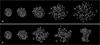 |
Fig. 1 Time evolution of rubble-pile aggregates. (a) Unstable configuration leading to breakup (ρb=1092 kg m−3, Ω=10−3 rad s−1). Snapshots taken at 0, 8, 16, 32, and 48 min. (b) Unstable configuration, but able to reshape to a new stable aggregate (ρb=1747 kg m−3, Ω=9×10⁻⁴ rad s−1). Snapshots taken at 0, 16, 56, 88, and 236 min. The time stamps refer to the physical time of the simulated scenario, not to the computational time. |
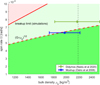 |
Fig. 2 Stable, unstable, and breakup regions in the (ρb − Ω) parameter space. With reference to the numerical simulations performed in this work, green and red regions denote initial conditions forming nondis-rupted and disrupted aggregates, respectively. The breakup transition is marked by the solid red line, and the theoretical limit for equilibrium reported in Eq. (3) is represented by the dashed red line. The intermediate region between the theoretical equilibrium and the breakup lines (light green area) includes aggregates that are not in equilibrium, but that are able to reshape without breaking apart. The vertical dashed blackline reports the maximum ρb value used in simulations. For reference, we report current (ρb − Ω) estimates (and their uncertainty) for asteroids Didymos (Naidu et al. 2020) and Moshup (Ostro et al. 2006). |
2.2 Theoretical framework
We considered a system of N-rigid bodies. The translational and rotational motion of each ith particle are described by the following equations of motion:
 (4)
(4)
 (5)
(5)
where ri is the position of the ith body, and mi is its mass. Equation (4) is written in an inertial frame centered on the barycenter of the system. The first term of the right-hand side represents the gravitational force that the ith particle receives from the N-body system, where G is the universal gravitational constant, rij is the relative position between the ith and jth particles defined as rj − ri, and rij- = ||rij||. The second and third terms of the right-hand side of Eq. (4) represent forces due to contact interaction between two different fragments. For body i, these forces act at contact points q, where Q is the total number of active contact points at a specific time step on the ith body. For each contact point q, we consider forces related to the visco-elastic behavior of the material (second term), and friction (third term). Both terms rely on properties of the material: coefficients of stiffness kiq and damping ciq in the first case, and the coefficient of friction ηiq in the last case. Furthermore, the resulting force is computed in a relevant local frame first (e.g., ξ is the local coordinate representing the displacement of the spring-dashpot system modeling the visco-elastic behavior of the material) and then transferred to the inertial frame using the transformation matrices  and
and  , which map the local frame into the common inertial frame. Equation (5) provides additional degrees of freedom to the problem by accounting for the rotational motion of each ith particle. In this case, the equation is written in the local frame attached to the rigid body particle, where Ii is its inertia matrix and ωi is its angular velocity vector. The last term of the right-hand side represents external torques due to off-center collisions or other contact-related interactions occurring at contact points q.
Overall, Eqs. (4) and (5) not only account for the N-body gravitational motion, but also for the granular dynamics between fragments, represented by contact and surface related forces, including dissipative terms. As anticipated, we refer to this problem as the granular N-body problem.
2.2.1 Global metrics
After clarifying the nature of the dynamical interactions into play within our granular N-body system, we provide here the mathematical definition of the chaotic indicators used in this work. We did not aim to identify the chaotic regions of the system, but started from the definitions used for different problems that can exhibit chaos. In the following, we therefore refer to the indicators computed as to chaotic indicators. More details for the interpretation of these indicators for the problem addressed here are given in the next section.
First of all, it is important to identify metrics that are able to inform us about the qualitative or quantitative behavior of the system. To this end, we identified two main classes of metrics providing information about the shape/mass distribution within the system and the energy content of the system. In particular, we used the polar moment of inertia of the system Ip and the inertia elongation λ as a measure of the shape/mass distribution. These are defined as
 (6)
(6)
 (7)
(7)
The polar moment of inertia Ip is the projection of the inertia tensor of the system I in the direction of the spin vector Ω of the system, and it is found by summing up the polar moments of inertia of all the particles in the system Iip (each projected on the Ω direction) using the Huygens-Steiner theorem. In Eq. (6), di is the distance between the two polar parallel axes centered on the barycenter of the system and on the barycenter of the ith body. Figure 3 shows two examples of the time evolution of the polar moment of inertia of the system for the cases reported in Fig. 1a (left, breakup case) and Fig. 1b (right, reshaping case). In these cases, the Ip(t) trajectory is shown to either diverge (breakup) or converge to a new value (reshaping). The inertia elongation λ was first defined in Ferrari et al. (2017) and represents the ratio of the minimum and maximum inertia moments of the system. Both these values, Ip and λ, provide information on the shape of the aggregate.
To quantify the energy content of the system, we used the total kinetic energy Ek and the pseudo-Jacobi potential J, defined as
 (8)
(8)
 (9)
(9)
Ek is the sum of translational and rotational kinetic energies of all N bodies of the system, where vi is the norm of the velocity vector of the ith body. The pseudo-Jacobi potential J is inspired by the Jacobi constant used in the context of the three-body problem (Szebehely 1967). It refers to the energy of a sample point with position rp and velocity vp in the corotating frame. In addition to the specific linear kinetic energy of the sample point, the pseudo-Jacobi potential accounts for the centrifugal contribution and the gravitational potential of the N masses, where rpi is the relative distance between the sample point and the ith body. We used J to evaluate the potential of a point located at the equator that corotates with the system. In this context, J provides a measure of whether a particle has sufficient energy to escape from the equator or if its motion is bounded within the system.
2.2.2 Indicators
We defined several indicators based on the global metrics identified above, and we use the notation W(t) to identify the trajectory (or time evolution) of one of the metrics, that is, either Ip(t), λ(t), Ek(t) or J(t). The trajectory W(t) was processed to compute four different classes of indicators: finite-time Lyapunov exponent (FTLE), lagrangian descriptor (LD), differential descriptor (DD), raw descriptor (RD).
The finite-time Lyapunov exponent is defined as
 (10)
(10)
where the asterisk subscript indicates a perturbed trajectory that separates from the nominal trajectory within the time frame between initial time t0 and a given time t1. The definition provided corresponds to the maximum local Lyapunov exponent, but we call it finite-time Lyapunov exponent because we analyze its performance at different values of tf. The so-defined FTLE quantifies the sensitivity of the trajectory W(t) to the parameters of the problem in a given time frame, and, by definition, it identifies chaotic motion (FTLE>0) versus nonchaotic motion (FTLE<0) within the system.
The lagrangian descriptor is defined as
 (11)
(11)
This definition is generalized from the original definition provided by Mancho et al. (2013), where LD is defined as the integral of a positive quantity. In practical terms, LD is a measure of the Euclidean arc-length of the trajectory in the given phase space and in the time interval between t0 and tf. In principle, trajectories with similar initial conditions will have a similar arc-length in the same time interval. In this respect, LD can give a similar conceptual information compared to the FTLE.
The differential descriptor is introduced in this work, defined as the derivative of the global metrics at a given time tf,
 (12)
(12)
Unlike FTLE and LD, this indicator is computed based on a single time information alone and provides instantaneous information about the system at tf, without any knowledge of its history. This is beneficial from a computational point of view, but it only provides information on the short-time evolution of the system. This can be used to assess whether W(t) increases, decreases, or is stable in time, and to quantify its variation rate in time. From the computational point of view, the derivative is computed by finite differences using the information from two (or three) consecutive time steps. The DD differs from the case of FTLE and LD, which are computed on large time intervals spanning several time steps.
The raw descriptor is also introduced in this work, defined as the raw metrics at a given time,
 (13)
(13)
Similar to the case of DD, this indicator only provides an instantaneous picture of the system. However, when compared to a reference or initial value W(t0), it can provide useful information on the current status of the system, also as regards specific geometrical features such as λ, and can act as a means of comparison between different configurations.
We provide here the rationale driving the selection of the four indicators. The first indicator is most frequently used in dynamical systems theory to reveal the invariant structures of a given system. In particular, for Hamiltonian systems, the computation of the Lyapunov exponent allows us to reveal equilibrium points, associated periodic and quasi-periodic orbits and hyperbolic manifolds, and the extension of the chaotic regions of the system. We therefore considered this as the first option to characterize the dynamical features of a granular system as well. The second indicator was developed in recent years and has been applied in different contexts as an alternative to the Lyapunov exponent because it is easier to formulate and has a similar capability to detect the invariant dynamical objects. Finally, the third and fourth indicators are a measure of the physical properties of the system, which are key to possible stability and transitions. They are thus considered for understanding how the system evolves as a whole.
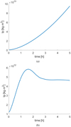 |
Fig. 3 Time evolution of the polar moment of inertia for the cases shown in Fig. 1a (breakup case) and Fig. 1b (reshaping case). Time refers to physical time of the simulated scenario, not to computational time. |
3 Results and discussion
We report the performance of the indicators defined in Sect. 2. We analyze the capability of each indicator to predict the dynamical outcome of the problem and to identify the dynamical transitions between a stable and an unstable aggregate. In particular, we build maps of the (ρb − Ω) configuration space using the indicators defined in Sect. 2, and we compare them to our ground-truth reference (Fig. 2), as discussed in Sect. 2. The performance of the indicators was assessed based on their capability to reproduce the three main dynamical regions in Fig. 2 and the transitions between them, either from a qualitative or from a quantitative point of view.
The granular N-body problem with dissipation is a nonau-tonomous, nonconservative system. In particular, the final configuration depends on the dynamical history of the aggregate. In this context, the properties of the system and the configuration space associated with them might vary significantly over time. We are interested in identifying the dynamical transitions that appear in the (ρb − Ω) configuration space. Therefore, we are interested both in the transient (to identify reshaping motion) and asymptotic (to identify breakup limit) behavior of the system, the latter being defined as the time after the transient phase has concluded, that is, when the system has reached an equilibrium configuration.
Figure 4 provides some examples of maps constructed using (from top row to bottom row) FTLE(Ip), DD(Ip) and RD(λ), RD(Ek), and their evolution up to three different instants of time along each row. Times refer to the physical time of the simulated scenario, not to computational time. We use these cases to show how the indicators were used and how the maps we obtained were interpreted. In particular, for a single map, the aim is to identify regions in which the contour levels can be associated with a different behavior or different regimes of motion. However, this can be done not only through contour levels in the maps that align with the breakup or equilibrium lines, but also with other structures, features, or regions that are clearly identifiable in the configuration map.
As mentioned, all maps vary in time until they reach an asymptotic condition (right column), in which the key elements of the map do not change any further. Referring to the examples of Fig. 4, we report here key takeaways.
The top row of Fig. 4 shows maps built using FTLE applied to the polar moment of inertia of the aggregate. As discussed in Sect. 2, the FTLE provides a direct measure of the level of chaos in the system. In the context of a spinning rubble-pile aggregate, we interpret chaotic motion (FTLE>0) as a behavior leading to breakup and nonchaotic motion (FTLE<0) as a behavior leading to a stable aggregate. The solid green lines in the FTLE plots indicate FTLE=0 levels. The first map (top left panel) shows the FTLE computed 16 min after the beginning of the simulation. At this time, two opposite regions of chaotic motion are identified for high spin rates (top left region of the map) and for low spin rates combined with high bulk densities (bottom right region of the map). These are related to motion occurring in the aggregate, where particles are pushed away from each other by a high spin rate, or conversely, they are pulled together by self-gravity. This is because the initial aggregate has been generated under different (ρb - Ω) conditions and therefore was in equilibrium under ρb = 1638 kg m−3 and Ω = 0 before the new ρb − Ω values of each configuration in the map were applied. For this reason, the blue region is stable, with very little particle motion, as the aggregate configurations here are more similar to those used to generate the initial aggregate. As the aggregate evolves in time, the bottom right chaotic region disappears, the top left region moves toward the ground-truth breakup limit (solid red line), and reaches it after approximately 2 h of simulation time. In this map, the reshaping realm can be seen as the region with FTLE < 0 up to the blue stable islands. Overall, FTLE(Ip) provides information on the qualitative dynamics of the system very early in time, identifying reshaping and particle relative motion. Most importantly, it provides a very precise estimate of the breakup limit curve before most aggregates have reached their equilibrium configuration.
The second row of Fig. 4 shows maps built using DD computed from the polar moment of inertia of the aggregate. Compared to the previous case, maps are more homogeneous. The last map (second row, right panel) shows a good alignment between the contour levels and the ground-truth breakup limit, showing a good capability to predict the qualitative behavior of the system. The DD = 0 line (solid green line) provides a separation between stable (where Ip(t) is constant in time) and unstable aggregates, providing a good estimate of the breakup limit, even though it requires longer simulation times than FTLE(Ip). In this case, the reshaping region is not clearly identified.
The third row of Fig. 4 shows maps built using RD computed from the inertia elongation of the aggregate. As for the previous case, the contour levels align toward the ground-truth breakup limit as the system evolves in time. The breakup limit is identified by a minimum in the map, which is stabilized after approximately 2 h of simulation time. This is consistent with the expected aggregate shapes: The minima of λ represent the more elongated aggregates, which are indeed found at the breakup limit. By definition of RD, the value of the indicator gives a direct information on the shape of the aggregate (inertia elongation) after a given time for each point in the (ρb − Ω) configuration.
The bottom row of Fig. 4 shows maps built using LD computed from the kinetic energy of the aggregate. At the beginning of the simulation, the map is very noisy, but it becomes more regular after a few hours. Eventually, some clear patterns emerge, some of which appear aligned to the breakup limit reference line. By definition, the LD(Ek) stores information about the history of the aggregate: A higher value of the indicator corresponds to higher values of the kinetic energy in the past. In this case, a region of higher particle motion is identified in the top left region of the map (breakup aggregates) and between the two reference lines (breakup limit and theoretical equilibrium), showing that these are the regions in which disruption and reshaping have occurred, respectively. Consistently, the reshaping region is identified with the region in which the level curves do not take a horizontal (stable domain) or a diagonal trend (unstable domain, beyond the breakup limit).
Figure 5 shows the final asymptotic map for all the other cases investigated. Maps with t = 300 min have not reached a stable asymptotic condition in this time frame and would require longer simulation times (or may never become stable).
Table 1 reports the performance of all the indicators we considered. In particular, we report the earliest time at which the breakup limit is clearly identified. We also include assessments whether the indicator provides information about the relative motion/reshaping behavior (i.e., if this information appears in the map) and if it provides a quantitative identification of the different dynamical regions (i.e., if the information can be unequivocally related to a range of parameters). In the last column, we evaluate the quality of the measure provided by the map on a three-level scale (1 – poor, 2 – good, and 3 – great) to provide information whether the map is affected by noise, or if the dynamical regions and their transitions are clearly identifiable (e.g., a rating of 3 would mean that the information can be extracted unequivocally from the map). We remark that this is a qualitative assessment only, with the goal to provide ground for a first comparison between different indicator/metrics combinations.
In summary, we note that maps constructed using shape-based metrics (Ip and λ) are smoother and allow an easier identification of the qualitative behavior leading to the breakup of the aggregate. On the other hand, maps constructed using energy-based metrics (Ek and J) focus more on capturing the transient relative motion within the system. Moreover, when they are associated with shape-based metrics, FTLE and DD provide a precise and rapid identification of the breakup limit, while LD and RD are slower in general and less effective in some cases. Conversely, LD and RD work better with energy-based metrics, but FTLE and DD do not perform well in this case. Finally, FTLE and LD are able to store information about the history of the aggregate, and DD and RD only provide an instantaneous picture of the system.
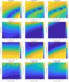 |
Fig. 4 Maps of the configuration space for a spinning rubble-pile aggregate using different indicators. Each row shows the evolution of a given map in time. The solid red line indicates the breakup limit derived from the granular N-body simulations (ground-truth reference), and the dashed red line indicates the theoretical equilibrium curve described by Eq. (3). The solid green line indicates level lines with FTLE(Ip) = 0 (first row) and DD(Ip) = 0 (second row). |
Performance of the indicators.
4 Conclusion
We presented a new method that is based on the exploitation of ad hoc indicators to identify dynamical transitions and characterize the qualitative behavior of a granular N-body system. The method was applied to a simple case study that focused on identifying the breakup limit for a spinning rubble-pile asteroid aggregate. The study systematically investigated the parameter space for a range of bulk densities and spin rates of the rubble-pile aggregate. The performance of several indicators based on both shape and energy content of the aggregate was assessed.
Although limited in scope, this work provides a first proof-of-concept of the method involving indicators. Some of them have shown a good capability to predict the fate of rubble-pile aggregates before they reached an equilibrium configuration. The maps we presented also provide a general and visual tool for characterizing the behavior of the system by capturing dynamical patterns, and by identifying the role of the parameters (bulk density and spin rate in this case), as well as the role of time in the evolution of rubble-pile aggregates. In this regard, this work represents a first step and determines the feasibility of the proposed approach, while more work is needed for a more detailed interpretation of the information provided by the maps and their evolution in time. The results presented here suggest that the method can be applied to more realistic rubble-pile models of asteroids, including those with higher resolution. Most importantly, the maps can provide insights into the relation between the fundamental properties of the system, its most relevant parameters, and their effects on the dynamics of the system. Examples are given by investigations of the role of parameters that are relevant to the rubble-pile stability problem, such as material properties, internal structure, cohesion, and on other dynamical scenarios, such as tidal deformation or binary formation. Finally, we envisage linking the results of the numerical maps with more theoretical approaches, such as that proposed in Scheeres (2020), or novel approaches that focus more on dynamical systems theory.
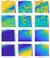 |
Fig. 5 Maps of the configuration space for a spinning rubble-pile aggregate using different indicators. Final asymptotic maps are shown for all the cases. Maps with t = 300 min have not reached a stable asymptotic condition in this time frame and would require longer simulation times (or may never become stable). The solid red line indicates the breakup limit derived from granular N-body simulations (ground-truth reference), and the dashed red line indicates the theoretical equilibrium curve described by Eq. (3). The solid green line indicates level lines with FTLE(W) = 0 (FTLE cases) and DD(W) = 0 (DD cases). |
Acknowledgements
F.F. acknowledges funding from the Swiss National Science Foundation (SNSF) Ambizione grant no. 193346. This work has been carried out within the framework of the NCCR PlanetS supported by the Swiss National Science Foundation. E.M.A. acknowledges the partial support received by Fondazione Cariplo through the program Promozione dell’attrattività e competitività dei ricercatori su strumenti dell’European Research Council - Sottomisura rafforzamento.
References
- Arakawa, M., Saiki, T., Wada, K., et al. 2020, Science, 368, 67 [NASA ADS] [CrossRef] [Google Scholar]
- Aranson, I.S., & Tsimring, L.S. 2001, Phys. Rev. E, 64, 020301 [NASA ADS] [CrossRef] [Google Scholar]
- Ballouz, R.-L., Walsh, K.J., Sánchez, P., et al. 2021, MNRAS, 507, 5087 [NASA ADS] [CrossRef] [Google Scholar]
- Banigan, E.J., Illich, M.K., Stace-Naughton, D.J., & Egolf, D.A. 2013, Nat. Phys., 9, 288 [NASA ADS] [CrossRef] [Google Scholar]
- Brisset, J., Cox, C., Anderson, S., et al. 2020, A&A, 642, A198 [NASA ADS] [CrossRef] [EDP Sciences] [Google Scholar]
- Chapman, C.R. 1978, in Asteroids: An Exploration Assessment, NASA Conf. Publ., 2053, 145 [Google Scholar]
- Farrés, A., Gao, C., Masdemont, J.J., et al. 2022, J. Guidance Control Dyn., 45, 1108 [CrossRef] [Google Scholar]
- Ferrais, M., Vernazza, P., Jorda, L., et al. 2020, A&A, 638, A15 [NASA ADS] [CrossRef] [EDP Sciences] [Google Scholar]
- Ferrari, F., & Tanga, P. 2020, Icarus, 350, 113871 [NASA ADS] [CrossRef] [Google Scholar]
- Ferrari, F., & Tanga, P. 2022, Icarus, 378, 114914 [NASA ADS] [CrossRef] [Google Scholar]
- Ferrari, F., Tasora, A., Masarati, P., & Lavagna, M. 2017, Multibody Syst. Dyn., 39, 3 [CrossRef] [Google Scholar]
- Ferrari, F., Lavagna, M., & Blazquez, E. 2020, MNRAS, 492, 749 [NASA ADS] [CrossRef] [Google Scholar]
- Fries, M., Abell, P., Brisset, J., et al. 2018, Acta Astronautica, 142, 87 [NASA ADS] [CrossRef] [Google Scholar]
- Goldhirsch, I. 2003, Annu. Rev. Fluid Mech., 35, 267 [NASA ADS] [CrossRef] [Google Scholar]
- Goodman, M.A., & Cowin, S.C. 1972, Arch. Rational Mech. Anal., 44, 249 [NASA ADS] [CrossRef] [Google Scholar]
- Hestroffer, D., Sánchez, P., Staron, L., et al. 2019, A&AR, 27, 6 [NASA ADS] [CrossRef] [Google Scholar]
- Holsapple, K. 2001, Icarus, 154, 432 [NASA ADS] [CrossRef] [Google Scholar]
- Holsapple, K.A. 2004, Icarus, 172, 272 [NASA ADS] [CrossRef] [Google Scholar]
- Holsapple, K.A. 2007, Icarus, 187, 500 [NASA ADS] [CrossRef] [Google Scholar]
- Holsapple, K.A. 2010, Icarus, 205, 430 [NASA ADS] [CrossRef] [Google Scholar]
- Holsapple, K.A., & Michel, P. 2006, Icarus, 183, 331 [NASA ADS] [CrossRef] [Google Scholar]
- Holsapple, K., Giblin, I., Housen, K., Nakamura, A., & Ryan, E. 2002, in Asteroids III, eds. W.F. Bottke Jr., A. Cellino, P. Paolicchi, & R.P. Binzel (University of Arizona Press), 443 [CrossRef] [Google Scholar]
- Jop, P., Forterre, Y., & Pouliquen, O. 2006, Nature, 441, 727 [NASA ADS] [CrossRef] [Google Scholar]
- Kleinfelter, N., Moroni, M., & Cushman, J.H. 2005, Phys. Rev. E, 72, 056306 [NASA ADS] [CrossRef] [Google Scholar]
- Koon, W.S., Lo, M.W., Marsden, J.E., & Ross, S.D. 2006, Dynamical Systems, the Three Body Problem and Space Mission Design (World Scientific) [Google Scholar]
- Korycansky, D., & Asphaug, E. 2006, Icarus, 181, 605 [NASA ADS] [CrossRef] [Google Scholar]
- Korycansky, D., & Asphaug, E. 2009, Icarus, 204, 316 [NASA ADS] [CrossRef] [Google Scholar]
- Laskar, J. 1989, Nature, 338, 237 [Google Scholar]
- Lauretta, D.S., DellaGiustina, D.N., Bennett, C.A., et al. 2019, Nature, 568, 55 [NASA ADS] [CrossRef] [Google Scholar]
- Lopesino, C., Balibrea-Iniesta, F., García-Garrido, V.J., Wiggins, S., & Mancho, A.M. 2017, Int. J. Bifurcation Chaos, 27, 1730001 [NASA ADS] [CrossRef] [Google Scholar]
- Mancho, A.M., Wiggins, S., Curbelo, J., & Mendoza, C. 2013, Commun. Nonlinear Sci. Numer. Simul., 18, 3530 [NASA ADS] [CrossRef] [Google Scholar]
- Michel, P., Benz, W., Tanga, P., & Richardson, D.C. 2001, Science, 294, 1696 [NASA ADS] [CrossRef] [Google Scholar]
- Michel, P., Benz, W., & Richardson, D.C. 2003, Nature, 421, 608 [NASA ADS] [CrossRef] [Google Scholar]
- Moeckel, R. 2016, Celest. Mech. Dyn. Astron., 128, 3 [Google Scholar]
- Movshovitz, N., Asphaug, E., & Korycansky, D. 2012, ApJ, 759, 93 [NASA ADS] [CrossRef] [Google Scholar]
- Naidu, S., Benner, L., Brozovic, M., et al. 2020, Icarus, 348, 113777 [CrossRef] [Google Scholar]
- Nedderman, R.M. 1992, Statics and Kinematics of Granular Materials, (Cambridge: Cambridge University Press) [CrossRef] [Google Scholar]
- Ostro, S.J., Margot, J.-L., Benner, L.A.M., et al. 2006, Science, 314, 1276 [NASA ADS] [CrossRef] [Google Scholar]
- Pfenniger, D. 2019, Celest. Mech. Dyn. Astron., 131 [Google Scholar]
- Portegies Zwart, S.F., Boekholt, T.C.N., Por, E.H., Hamers, A.S., & McMillan, S.L.W. 2022, A&A, 659, A86 [NASA ADS] [CrossRef] [EDP Sciences] [Google Scholar]
- Rozitis, B., MacLennan, E., & Emery, J.P. 2014, Nature, 512, 174 [CrossRef] [Google Scholar]
- Scheeres, D.J. 2012, Celest. Mech. Dyn. Astron., 113, 291 [NASA ADS] [CrossRef] [Google Scholar]
- Scheeres, D.J. 2016, Celest. Mech. Dyn. Astron., 128, 131 [Google Scholar]
- Scheeres, D.J. 2018, Celest. Mech. Dyn. Astron., 130, 55 [NASA ADS] [CrossRef] [Google Scholar]
- Scheeres, D.J. 2020, Celest. Mech. Dyn. Astron., 132, 5 [NASA ADS] [CrossRef] [Google Scholar]
- Scheeres, D.J., Hsiao, F.-Y., & Vinh, N.H. 2003, J. Guidance Control Dyn., 26, 62 [NASA ADS] [CrossRef] [Google Scholar]
- Sunday, C., Murdoch, N., Wilhelm, A., et al. 2021a, MNRAS, 498, 1062 [Google Scholar]
- Sunday, C., Zhang, Y., Thuillet, F., et al. 2021b, A&A, 656, A97 [NASA ADS] [CrossRef] [EDP Sciences] [Google Scholar]
- Szebehely, V. 1967, Theory of Orbits: The Restricted Problem of Three Bodies (New York and London: Academic Press) [Google Scholar]
- Thuillet, F., Zhang, Y., Michel, P., et al. 2021, A&A, 648, A56 [NASA ADS] [CrossRef] [EDP Sciences] [Google Scholar]
- Turuban, R., Lester, D.R., Heyman, J., Borgne, T.L., & Méheust, Y. 2019, J. Fluid Mech., 871, 562 [NASA ADS] [CrossRef] [Google Scholar]
- Wada, K., Ishibashi, K., Kimura, H., et al. 2021, A&A, 647, A43 [NASA ADS] [CrossRef] [EDP Sciences] [Google Scholar]
- Walsh, K.J., Richardson, D.C., & Michel, P. 2008, Nature, 454, 188 [NASA ADS] [CrossRef] [Google Scholar]
- Watanabe, S., Hirabayashi, M., Hirata, N., et al. 2019, Science, eaav8032 [Google Scholar]
- Wensrich, C., & Katterfeld, A. 2012, Powder Technol., 217, 409 [Google Scholar]
- Zhang, Y., & Lin, D.N.C. 2020, Nat Astron., 4, 852 [NASA ADS] [CrossRef] [Google Scholar]
- Zhang, Y., Richardson, D.C., Barnouin, O.S., et al. 2017, Icarus, 294, 98 [NASA ADS] [CrossRef] [Google Scholar]
- Zhang, Y., Michel, P., Richardson, D.C., et al. 2021, Icarus, 114433 [NASA ADS] [CrossRef] [Google Scholar]
- Zhong, J., & Ross, S.D. 2021, Nonlinear Dyn., 104, 3109 [Google Scholar]
1092, 1201, 1310, 1419, 1529, 1638, 1747, 1856, 1965, 2075, and 2184 kg s−1.
1, 2, 3, 4, 5, 6, 7, 8, 9, and 10 e–4 rad s−1.
All Tables
All Figures
|
Fig. 1 Time evolution of rubble-pile aggregates. (a) Unstable configuration leading to breakup (ρb=1092 kg m−3, Ω=10−3 rad s−1). Snapshots taken at 0, 8, 16, 32, and 48 min. (b) Unstable configuration, but able to reshape to a new stable aggregate (ρb=1747 kg m−3, Ω=9×10⁻⁴ rad s−1). Snapshots taken at 0, 16, 56, 88, and 236 min. The time stamps refer to the physical time of the simulated scenario, not to the computational time. |
| In the text | |
|
Fig. 2 Stable, unstable, and breakup regions in the (ρb − Ω) parameter space. With reference to the numerical simulations performed in this work, green and red regions denote initial conditions forming nondis-rupted and disrupted aggregates, respectively. The breakup transition is marked by the solid red line, and the theoretical limit for equilibrium reported in Eq. (3) is represented by the dashed red line. The intermediate region between the theoretical equilibrium and the breakup lines (light green area) includes aggregates that are not in equilibrium, but that are able to reshape without breaking apart. The vertical dashed blackline reports the maximum ρb value used in simulations. For reference, we report current (ρb − Ω) estimates (and their uncertainty) for asteroids Didymos (Naidu et al. 2020) and Moshup (Ostro et al. 2006). |
| In the text | |
|
Fig. 3 Time evolution of the polar moment of inertia for the cases shown in Fig. 1a (breakup case) and Fig. 1b (reshaping case). Time refers to physical time of the simulated scenario, not to computational time. |
| In the text | |
|
Fig. 4 Maps of the configuration space for a spinning rubble-pile aggregate using different indicators. Each row shows the evolution of a given map in time. The solid red line indicates the breakup limit derived from the granular N-body simulations (ground-truth reference), and the dashed red line indicates the theoretical equilibrium curve described by Eq. (3). The solid green line indicates level lines with FTLE(Ip) = 0 (first row) and DD(Ip) = 0 (second row). |
| In the text | |
|
Fig. 5 Maps of the configuration space for a spinning rubble-pile aggregate using different indicators. Final asymptotic maps are shown for all the cases. Maps with t = 300 min have not reached a stable asymptotic condition in this time frame and would require longer simulation times (or may never become stable). The solid red line indicates the breakup limit derived from granular N-body simulations (ground-truth reference), and the dashed red line indicates the theoretical equilibrium curve described by Eq. (3). The solid green line indicates level lines with FTLE(W) = 0 (FTLE cases) and DD(W) = 0 (DD cases). |
| In the text | |
Current usage metrics show cumulative count of Article Views (full-text article views including HTML views, PDF and ePub downloads, according to the available data) and Abstracts Views on Vision4Press platform.
Data correspond to usage on the plateform after 2015. The current usage metrics is available 48-96 hours after online publication and is updated daily on week days.
Initial download of the metrics may take a while.