| Issue |
A&A
Volume 667, November 2022
|
|
|---|---|---|
| Article Number | A80 | |
| Number of page(s) | 15 | |
| Section | Cosmology (including clusters of galaxies) | |
| DOI | https://doi.org/10.1051/0004-6361/202244100 | |
| Published online | 09 November 2022 | |
Baryon acoustic oscillations from a joint analysis of the large-scale clustering in Fourier and configuration space
Aix-Marseille Univ., CNRS/IN2P3, CPPM, Marseille, France
e-mail: This email address is being protected from spambots. You need JavaScript enabled to view it.
, This email address is being protected from spambots. You need JavaScript enabled to view it.
Received:
24
May
2022
Accepted:
7
August
2022
Abstract
Baryon acoustic oscillations (BAOs) are a powerful probe of the expansion history of our Universe and are typically measured in the two-point statistics of a galaxy survey, either in Fourier space or in configuration space. In this work, we report a first measurement of BAOs from a joint fit of power spectrum and correlation function multipoles. We tested our new framework with a set of 1000 mock catalogs and showed that our method yields smaller biases on BAO parameters than individually fitting power spectra or correlation functions, or when combining them with the Gaussian approximation method. Our estimated uncertainties are slightly larger than those from the Gaussian approximation, likely due to noise in our sample covariance matrix, the larger number of nuisance parameters, or the fact that our new framework does not rely on the assumption of Gaussian likelihoods for the BAO parameters. However, we argue that our uncertainties are more reliable since they rely on fewer assumptions, and because our method takes correlations between Fourier and configuration space at the level of the two-point statistics. We performed a joint analysis of the luminous red galaxy sample of the extended baryon oscillation spectroscopic survey (eBOSS) data release 16, obtaining DH/rd = 19.27 ± 0.48 and DM/rd = 17.77 ± 0.37, in excellent agreement with the official eBOSS consensus BAO-only results DH/rd = 19.33 ± 0.53 and DM/rd = 17.86 ± 0.33.
Key words: cosmological parameters / large-scale structure of Universe
© T. Dumerchat and J. E. Bautista 2022
 Open Access article, published by EDP Sciences, under the terms of the Creative Commons Attribution License (https://creativecommons.org/licenses/by/4.0), which permits unrestricted use, distribution, and reproduction in any medium, provided the original work is properly cited.
This article is published in open access under the Subscribe-to-Open model. This email address is being protected from spambots. You need JavaScript enabled to view it. to support open access publication.
1. Introduction
The study of the accelerated nature of the expansion of the Universe has seen significant progress in the past decade thanks to measurements of baryon acoustic oscillations (BAOs) in the three-dimensional distribution of galaxies. Similarly to type-Ia supernovae (see Brout et al. 2022 and references therein for the latest results), BAO measurements have shown that the expansion is accelerating, imposing the need of a dark energy component in the energy budget of the Universe. The next decade will see a large flow of data coming from galaxy surveys whose goal is the precise measurement of BAO over a large span of the cosmic history.
The latest BAO measurements from spectroscopic surveys were produced by the cosmological component of the fourth generation of the Sloan Digital Sky Survey (SDSS-IV, Blanton et al. 2017), named the extended Baryon Oscillation Spectroscopic Survey (eBOSS, Dawson et al. 2016). The eBOSS project produced measurements of BAO using luminous red galaxies at an effective redshift zeff = 0.7 (Bautista et al. 2021; Gil-Marín et al. 2020), using emission line galaxies at zeff = 0.85 (Raichoor et al. 2021; Tamone et al. 2020; de Mattia et al. 2021), using quasars as tracers of the matter field at zeff = 1.48 (Hou et al. 2021; Neveux et al. 2020), and quasars with visible Lyman-α forests at zeff = 2.33 (du Mas des Bourboux et al. 2020). Two additional lower redshift measurements were made at zeff = 0.38 and 0.51 from the third generation of SDSS, BOSS (Eisenstein et al. 2011; Dawson et al. 2013; Alam et al. 2017). At zeff = 0.15, we have measurements from the SDSS-II Main Galaxy Sample (Ross et al. 2015a; Howlett et al. 2015). Measurements from other surveys include the 6dFGS (Beutler et al. 2011) at zeff = 0.10 and the WiggleZ Dark Energy Survey (Kazin et al. 2014) with three redshift bins spanning 0.2 < z < 1.0. The latest BAO measurements from photometric surveys were produced by the Dark Energy Survey (DES, DES Collaboration 2016). DES produced angular BAO measurements in five redshift intervals between 0.6 and 1.1 using three years of its data (DES Collaboration 2021).
Baryon acoustic oscillation measurements have traditionally been performed in configuration space and/or in Fourier space. Configuration space analysis is based on estimates of correlation function ξ as a function of separation r, commonly done with pair-counting techniques. Fourier space analyses assign galaxies into a regular grid so as to Fourier transform it in order to compute the power spectrum multipoles Pℓ as a function of wavevector k. Both types of analyses perform a statistical measurement starting from the exact same dataset, defined as a list of angular positions, redshifts, and weights, as well as some definition of the window function of the survey which is often a purely Poisson set of points following the same angular and redshift distribution as the real data. In principle, both types of analyses should yield the same cosmological constraints since they have a common starting point. In practice, choosing a limited range of scales used when fitting models slightly breaks this perfect degeneracy. Noise properties or systematic effects on the estimated (and binned) statistics also differ between ξ(r) and P(k). The models of clustering used to fit two-point functions also commonly differ, that is to say when performing a full shape analysis the clustering models in configuration space can differ from just a Fourier transform of those in Fourier space. All these differences slightly reduce the correlations to levels below 100%. As an example, Bautista et al. (2021) show using the best-fit values for the dilation parameters on an ensemble of mock catalogs that BAO results in configuration and Fourier spaces are roughly 90% correlated, for their particular choices of scales and models. Recent analysis of BAO and redshift-space distortions (RSD) usually combine results from configuration and Fourier space analyses into a single consensus result.
Given that the correlations between cosmological results are not exactly 100% between configuration and Fourier space analyses, there is a slight statistical gain in producing a combined result. Systematic errors might as well be reduced by this combination, since they may manifest themselves differently in both spaces. In collaboration working groups, often two or more teams produce their analyses in a single space, making it difficult to decide which results to quote as final. Therefore, there are several advantages to produce joint results between Fourier and configuration spaces.
When calculating a consensus result, it is important to correctly take into account the strong correlations between measurements in configuration and Fourier space. Sánchez et al. (2017) described a method to compute a consensus result, which was used for the first time in SDSS-III BOSS (Alam et al. 2017) and extended to the latest measurements from SDSS-IV eBOSS survey. This method was used to produce consensus results on BAO and RSD analyses of a given survey, yielding constraints on DH/rd, DM/rd and fσ8, where DH is the Hubble distance c/H, DM is the comoving angular diameter distance, rd is the comoving sound horizon at drag epoch (the BAO scale), f is the growth-rate of structures and σ8 is the normalization of the smoothed linear matter power spectrum. However, the method from Sánchez et al. (2017) assumes that the individual likelihoods on BAO parameters are Gaussian, which is not necessarily true, particularly in a regime of low signal-to-noise ratio.
In this work, we developed a framework to perform simultaneous BAO analyses in both configuration and Fourier spaces. The advantages of our framework over past work are (1) individual likelihoods on BAO parameters from each space are not assumed to be Gaussian, (2) the resulting posterior distribution is not necessarily Gaussian, resulting in more reliable uncertainties, (3) it is simpler, and (4) yields smaller systematic biases. Our method only relies on a sufficiently good estimate of the full covariance matrix, particularly the cross-covariance between two-point functions in Fourier and configuration spaces. We validated our method on realistic mock catalogs and performed comparison with previous work.
This paper is organized as follows. In Sect. 2, we describe the dataset used to validate our methods. In Sect. 3, we introduce the BAO modeling, which is mostly the same used in Bautista et al. (2021), Gil-Marín et al. (2020), as well as the methods to produce consensus results. Section 4 presents several statistical and systematical tests of both methods and finally the application on real data on Sect. 5.
2. Dataset
To validate our methodology, we used 1000 mock catalogs reproducing the Luminous Red Galaxy (LRG) sample from the eBOSS survey, though our methods are not survey specific. This dataset is the same employed in the cosmological analyses of Bautista et al. (2021), Gil-Marín et al. (2020), and we refer the reader to these references for further details.
2.1. The eBOSS survey
The extended Baryon Oscillation Spectroscopic Survey (eBOSS, Dawson et al. 2016) was a 5-year observing program using multiobject fiber-fed spectrographs (Smee et al. 2013) mounted on the focal plane of the 2.5 m Sloan Foundation Telescope (Gunn et al. 2006) at the Apache Point Observatory. During eBOSS, 174 816 LRG redshifts were obtained over 4242 deg2 of both northern and southern skies, in the redshift interval 0.6 < z < 1.0. These were combined with BOSS galaxies in the same redshift range covering 9493 deg2 of sky, resulting in a total of 377 458 LRG redshifts (Ross et al. 2020). The survey geometry was defined using a set of randomly distributed points, taking into account masked areas. The final data sample has correction weights accounting for the photometric and spectroscopic incompleteness, as well as some spurious correlations (e.g., with stellar density, Galactic extinction). The final catalog is the basis for mock catalog production.
2.2. Mock catalogs
In this work we use a sample of 1000 mock realizations of the eBOSS LRG sample to validate our methodology and to perform statistical tests. A set of 1000 realisations of the eBOSS LRG survey were produced using the EZMOCK method (Chuang et al. 2015), which employs the Zel’dovich approximation to compute the density field at a given redshift. This method is faster than n-body simulations and has been calibrated to reproduce the two- and three-point statistics of the given galaxy sample, to a good approximation and up to mildly nonlinear scales. The angular and redshift distributions of the eBOSS LRG sample were reproduced, including both photo and spectro-incompleteness effects as well as systematic effects introducing spurious correlations. These mocks aim to include all known features in real data. A detailed description of the EZMOCKS can be found in Zhao et al. (2021). These mocks were used in this work to estimate covariance matrices and to perform statistical studies of our method. As we will describe in Sect. 3.4, mocks are also required by the Gaussian approximation method for combining configuration and Fourier space results into a single consensus result.
3. Methodology
3.1. Measuring the clustering
We used correlation function and power spectrum multipoles estimated for each of the 1000 EZMOCK realisations. The correlation function is estimated using the Landy & Szalay (1993) estimator, while power spectra were calculated using the Yamamoto et al. (2006) estimator, as implemented by Bianchi et al. (2015), Scoccimarro (2015).
We attempt to remove the impact of non-linear evolution of galaxies and a fraction of redshift-space distortions by applying the reconstruction technique of Burden et al. (2015). Using the density field itself, we estimate the displacements using the Zeldovich approximation to move the galaxies “back in time”. This technique increases the precision of the measurement by sharpening the BAO feature. According to Carter et al. (2020) the BAO results are not sensitive to small variations in the cosmology used to perform the reconstruction. In Appendix B, we performed the analysis for the prereconstructed sample, where we derive the same conclusions as for the postreconstruction cases (though at lower signal-to-noise ratios).
3.2. BAO modelling
The models used in this work are the same employed in Bautista et al. (2021), Gil-Marín et al. (2020), which are themselves based on previous work (Alam et al. 2017; Gil-Marín et al. 2016, 2018; Ross et al. 2017; Bautista et al. 2018). We briefly summarize these models here. The code that produces the model and perform the fitting to the data is publicly available1.
The aim is to model both the power spectrum Pℓ(k) and correlation function multipoles ξℓ(r) as a function of wave-number k and separations r, respectively, where ℓ is the order of the multipole expansion. We focus on scales relevant for the measurement of the baryon acoustic oscillation (BAO) feature, typically 0 < k < 0.3 h−1 Mpc for power-spectrum and 30 < r < 180 h−1 Mpc for correlation function.
The starting point is a linear-theory-based model for the redshift-space anisotropic galaxy power-spectrum P(k, μ),
![Mathematical equation: $$ \begin{aligned} P(k, \mu _k) =&\frac{b^2 \left[1+\beta (1-S(k))\mu _k^2\right]^2}{(1+ k^2\mu _k^2\Sigma _{\rm s}^2/2)}\nonumber \\&\times \left[P_{\rm no \, peak}(k) + P_{\rm peak}(k) e^{-k^2\Sigma _{\rm nl}^2(\mu _k)/2}\right], \end{aligned} $$](/articles/aa/full_html/2022/11/aa44100-22/aa44100-22-eq1.gif) (1)
(1)
where b is the linear density bias of the galaxy population, β is the redshift-space distortions parameter defined as the ratio between the growth-rate f and b, k is the modulus of the wave-vector k and μk is the cosine of the angle between the wave-vector and the line of sight. The broadening of the BAO peak caused by non-linear clustering is reproduced by applying an anisotropic Gaussian smoothing, that is by multiplying the “peak-only” power spectrum Ppeak (see below) by a Gaussian function with dispersion given by  . The non-linear random motions on small scales are modeled by a Lorentzian distribution parametrized by Σs.
Following Seo et al. (2016), the term  for the postreconstruction model and S(k)=0 for the prereconstruction, where Σr = 15 h−1 Mpc is the smoothing parameter used when reconstructing the galaxy catalogs.
We follow the procedure from Kirkby et al. (2013) to decompose the BAO peak component Ppeak from the full linear power-spectrum Plin. We start by computing the correlation function by Fourier transforming Plin, then we replace the correlations over the peak region by a polynomial function fitted using information outside the peak region (50 < r < 80 and 160 < r < 190 h−1 Mpc). The resulting correlation function is then Fourier transformed back to get Pno peak. The linear power spectrum Plin is obtained from CAMB2 (Lewis et al. 2000) with cosmological parameters of our fiducial cosmology defined in Table 1.
Fiducial cosmologies used in this work.
The multipoles of the power-spectrum Pℓ(k) are obtained by integrating over μk weighted by the Lengendre polynomials Lℓ(μk):
 (2)
(2)
The correlation function multiples ξℓ(r) are obtained by Hankel transforming the Pℓ(k):
 (3)
(3)
where jℓ are the spherical Bessel functions. These transforms are computed using HANKL3 that implements the FFTLog algorithm by Hamilton (2000).
The BAO peak position is parametrised via two dilation parameters, one scaling separations across the line of sight, α⊥, and one scaling separations along the line of sight, α∥. The observed k is related to the true k′ by  and k⊥ = k′/α⊥. Therefore, the observed power spectrum relates to the true power spectrum as
 (4)
(4)
We note that this volume scaling does not apply for the correlation function:
 (5)
(5)
These BAO dilation parameters are related, respectively, to the comoving angular diameter distance, DM = (1 + z)DA(z), and to the Hubble distance, DH = c/H(z), by
 (6)
(6)
 (7)
(7)
where rd is the comoving sound horizon at drag epoch, and zeff is the effective redshift of the survey. The rd rescaling is here to account for the choice of template cosmology used to compute the fixed linear power spectrum. For simplicity, the template cosmology is chosen to match the fiducial cosmology used to estimate distances from redshifts.
We apply the scaling factors exclusively to the peak component of the power spectrum Ppeak(k), effectively removing any dependency of these parameters on the smooth part Pno peak(k) (Kirkby et al. 2013).
In order to properly marginalize over any mis-modelling of the smooth part of Pℓ(k) and ξℓ(r), we add to our model a linear combination of smooth functions of scale, with free amplitudes to be marginalised over. These smooth functions can also account for potential unknown systematic correlations that contaminating our measurements. Furthermore, since there are no accurate analytical models for correlations postreconstruction (the S(k) term in Eq. (1) is generally not sufficient), these smooth functions can also account for this mis-modelling. As these smooth functions are highly correlated with the finger of god Lorentzian, we fix the parameter Σs to zero. Our final template can be written as:
 (8)
(8)
 (9)
(9)
where  and
and  are the amplitudes for each power i of scale, k or r, and multipole order ℓ. In Gil-Marín et al. (2020), the BAO analysis in Fourier space used (imin, imax)=(−1, 1), while in Bautista et al. (2021) the configuration space analysis used (imin, imax)=(−2, 0). For both, this corresponds to three free parameters per multipole. In this work, our baseline choice is (imin, imax)=(−2, 1) when performing joint fits unless stated otherwise.
Our baseline BAO analysis uses the monopoles P0, ξ0 and quadrupoles P2, ξ2 of the power spectrum and correlation functions (see Appendix A for results using the hexadecapole). We fix β = 0.35 and fitting b with a flat prior between b = 1 and 4. For all fits, the broadband parameters are free, while both dilation parameters are allowed to vary between 0.5 and 1.5.
3.3. Parameter inference
The cosmological parameter inference is performed by means of the likelihood analysis of the data. The likelihood ℒ is defined such that
 (10)
(10)
where θ is the vector of parameters, Δ is a vector containing residuals between observed multipoles and their model, Np is the total number of elements in Δ. An estimate of the precision matrix  is obtained from the unbiased estimate of the covariance from 1000 realisation of EZmocks:
  where
where  is the measured Pℓ(ki) or ξℓ(ri) for the kth realisation. The factor D = (Np + 1)/(Nmocks − 1) accounts for the skewed nature of the Wishart distribution (Hartlap et al. 2007).
The best-fit BAO parameters (α⊥, α∥) are determined by minimizing χ2 of Eq. (10) using a quasi-Newton minimum finder algorithm IMINUIT4 which marginalizes over nuisance parameters while sampling for the parameters of interest. The uncertainties in α∥ and α⊥ are estimated with the MINOS function provided by IMINUIT. This functions computes the intervals where χ2 increases by unity, which corresponds to a 68% confidence interval. Gaussianity is not assumed in this calculation and uncertainties can be asymmetric with respect to the best-fit value. The two-dimensional confidence contours in (α⊥, α∥), are estimated using the CONTOUR function from IMINUIT. Similarly to MINOS, this function scans χ2 values in two dimensions, looking for the contours yielding a Δχ2 = 2.3 or 5.9 for 68 and 95% confidence levels, respectively.
3.4. Consensus via Gaussian approximation
In previous work, configuration and Fourier space results were combined into a single consensus result using the method presented in Sánchez et al. (2017).
The idea of the method is to generate a consensus result from M different measurement vectors xm, each containing p elements, and their covariance matrices Cmm, each of size p × p. For example, we want to combine M = 2 measurements of the vector xm = [α⊥, α∥] containing p = 2 parameters from Fourier (m = 1) and configuration space (m = 2), each with its own 2 × 2 error matrix Cmm derived from their posteriors. The consensus is a single vector xc with covariance Cc, for which the expressions assume that the χ2 between individual measurements is the same as the one from the consensus result. The expression for the combined covariance matrix is
 (11)
(11)
and the combined data vector is
 (12)
(12)
where Cmn is a p × p block from the full covariance matrix between all parameters and methods 𝒞, containing pM × pM elements, defined as
 (13)
(13)
The diagonal blocks Cmm come from each measurement method M, therefore, assuming Gaussian likelihoods for the p parameters. The off-diagonal blocks Cmn with m ≠ n cannot be in principle estimated from the data itself. These off-diagonal blocks are commonly built from mock catalogs. Using a set of many realisations, one can build 𝒞 from all the realisations of xm for each method. We obtain the correlation coefficients  , that is the covariance 𝒞 normalized by its diagonal elements, between parameters p1, p2 and methods m, n. We scale these coefficients by the diagonal errors from the data, to obtain the final matrix 𝒞 for the data.
It is worth emphasizing that the matrix 𝒞 for our data, and more specifically its off-diagonal blocks, depend on that particular realisation of the data in principle. However, the ones derived from mock measurements are ensemble averages. We account for this fact by scaling the correlations coefficients from the mocks in order to match the maximum correlation coefficient that would be possible with the data (Ross et al. 2015b). For the same parameter p1 measured by two different methods m and n, we assume that the maximum correlation between them is given by ρmax = σp1, m/σp1, n, where σp is the error of parameter p. This number is computed for the data realisation  and for the ensemble of mocks
  . We can write the adjusted correlation coefficients for one particular realisation as
 (14)
(14)
The equation above accounts for the diagonal terms of the off-diagonal block Cmn. For the off-diagonal terms, we use
 (15)
(15)
This adjustment of correlation coefficients is an addition to the method proposed by Sánchez et al. (2017) and was first implemented in Bautista et al. (2021) to obtain consensus results.
In summary, the method proposed by Sánchez et al. (2017) can provide consensus results from strongly correlated measurements of the same quantities. However, it assumes Gaussian likelihoods and yields Gaussian posteriors on the final parameters, which is not a good approximation when measurements are noisy. Also, it relies on mock measurements twice: once to derive the covariance matrix of two-point functions, from which we derive each parameter vector xm; and once again to derive the full parameter-method covariance 𝒞, using Eqs. (14) and (15). We call this method Gaussian approximation (GA). In the following section, we study joint fits in Fourier and configuration space, such that mock catalogs are used only once to derive a consensus result.
3.5. Joint analysis
We studied a new alternative method to get a unique set of constraints on the parameters α∥ and α⊥, taking into account the full correlations between the configuration space (CS) and Fourier space (FS) measurements. We refer to this method as Joint Space (JS) analysis. We concatenate the measured ξℓ multipoles with the Pℓ multipoles such that we obtain a data vector [ξ0,ξ2,P0,P2] with (2×rbins+2×kbins) data points. We then fit the data using a unique set of parameters, except for the nuisance parameters defining the polynomial smooth functions (Eqs. (8) and (9)).
In order to perform the joint inference, one needs to estimate the full covariance matrix. We use the measured Pℓ and ξℓ on the 1000 EZmocks to compute the covariance matrix  . As in Bautista et al. (2021) and Gil-Marín et al. (2020), we apply the following scale cuts: r ∈ [50, 150] h−1 Mpc and k ∈ [0.02, 0.3] h−1 Mpc. Figure 1 shows the resulting correlation matrix, defined as
 ![Mathematical equation: $ \boldsymbol{R} = \boldsymbol{\sigma}^{-1}\boldsymbol{\hat{C}}[\boldsymbol{\sigma}^{-1}]^T $](/articles/aa/full_html/2022/11/aa44100-22/aa44100-22-eq28.gif) , where σ is the vector composed by the square-root of the diagonal elements of
, where σ is the vector composed by the square-root of the diagonal elements of  . The diagonal blocks show the well-known correlations between the monopole and quadrupole in the same space, while the off diagonal blocks reveal the correlation patterns between the two spaces. The correlations between the two spaces monopole-monopole and quadrupole-quadrupole present the same non-linear features. A given physical scale r is correlated (and anti-correlated) with several k modes, meaning that the statistical information contained in a given scale is spread out over several spectral modes. A physical modeling of these features is proposed in Appendix C.
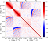 |
Fig. 1. Correlation matrix of the correlation function ξℓ and power spectrum multipoles Pℓ estimated using the 1000 independent measurements of EZmocks. |
We then need an estimate for the precision matrix  in Eq. (10). Inverting the covariance mixes the different modes and scales across CS and FS. The top panel of Fig. 2 presents the resulting correlations in the normalized precision matrix (for convenience we call the coefficients of the precision matrix ‘correlations’). Green arrows indicate the regions detailed in the bottom panels, where we focus on the correlations between the CS ξ2 and the FS P0 and P2, respectively by ploting the amplitude of the precision matrix at two fixed scaled rmin = 52.5 h−1 Mpc and rmax = 147.5 h−1 Mpc. The error bars of the precision matrix are computed according to Eq. (29) of Taylor et al. (2013). We see that at both scales, ξ2 is weakly correlated with P0 while being strongly correlated with P2. This result is in agreement with the correlations between ξ0 and ξ2. Furthermore, for large r, while the number of correlated k modes increases, the amplitude of the correlations decreases distinctly for ξ2 − P2, and increases for ξ2 − P0. Note that the correlations between the ξ0 and Pℓ are not shown here but behave in a similar fashion.
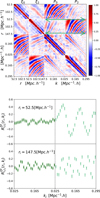 |
Fig. 2. Precision matrix of the correlation function ξℓ and power spectrum multipoles Pℓ. Top panel: normalized estimated precision matrix |

While capturing additional information about the scale dependence of the joint space correlations, our new methodology has some drawbacks. Indeed, because the covariance matrix  we use to infer our set of parameters is an estimate of the real precision matrix drawn from a Wishart distribution (finite sample of mocks), each element is affected by its own uncertainty that should be correctly propagated to the uncertainty of the estimated parameters. It has been shown in Dodelson & Schneider (2013) that this additional “noise” is directly proportional to the parameter covariance. We therefore need to apply correction factors to the obtained Cθ. These factors are given in Percival et al. (2014) as:
 (16)
(16)
with D the Hartlap factor defined in Sect. 3.3 and
 (17)
(17)
Note that this is also true for a classic FS or CS analysis but since the correction factors only scale with the number of parameters, data bins and mocks used to estimate the covariance, the enlargement on the constraints is smaller. The factor m1 is to be directly applied to the estimated parameter covariance matrix for a given measurement, while the factor m2 scales the standard deviation of a given parameter over a set of mocks. The values of the parameters m1 and m2 are given in Table 2. Since the enlargement of the parameter constraints ( ) expected in CS is about 1%, 1.7% in FS and 3% in JS, we expect slightly looser constraints for the joint analysis.
Correction factors for the three analysis performed in this work.
4. Results on mock catalogs
In this section, we use postreconstruction EZMOCKS to validate our parameter inference and error estimation (see Appendix B for a discussion on the analysis of the prereconstruction EZMOCKS). The aim is to compare results from configuration space (CS), Fourier space (FS), Joint space (JS) with the consensus results from the Gaussian approximation (GA).
4.1. Fits on average correlations
Using the inference methodology described in the Sect. 3, we fit the average Pℓ and ξℓ of the 1000 EZmocks in order to study potential biases and compare the GA and JS methods.
At first, we model ξℓ and Pℓ in the separation ranges r ∈ [50, 150] h−1 Mpc and k ∈ [0.02, 0.3] h−1 Mpc, by setting the broad band smooth polynomial functions from Eqs. (8) and (9) to the shape (imin, imax)=(−2, 1) and letting all fitting parameters free. Then, we assess the robustness of the best fit parameters with respect to variations in Σ⊥, Σ∥, k ranges, r ranges, number of broadband terms, and template cosmology for the linear power spectrum. Each time we vary one of those settings we keep the other ones fixed in all spaces (CS, FS and JS), facilitating the comparisons of results. Since we fit the mean of the mocks, we normalize the covariance matrix by the total number of mocks Nmocks = 1000. As the covariance is estimated with the same 1000 realisations, we do not expect it to be highly accurate, but sufficient for our purposes.
Figure 3 presents the impact of different analysis settings on the best fit values of α∥ and α⊥ for the GA (in black) and JS (in green) analysis. In every plot, a gray shaded area represents the 1 percent deviation from the expected value, which was the tolerance used in previous analysis. First, we tested different set of values for the broadening of the BAO peak, (Σ∥, Σ⊥), corresponding to the best values found in CS (7.90, 5.58), FS (7.23, 4.72) and JS (7.43, 5.21), all in units of h−1 Mpc. Both GA and JS analyses are robust to changes in those parameters. Both GA and JS analyses are also robust for different ranges of scales used in the fit, presenting small and coherent shifts. This indicates that the information is correctly extracted only from the BAO feature. When varying the broadband terms, the JS method shows stable results except for α∥ in one setting (−1, 1), where the broadband is not flexible enough to fit the residuals. When increasing the number of polynomial terms, the systematic shifts are notably smaller in JS than GA. The last two panels of Fig. 3 show the influence of the template cosmology used to compute the linear power spectrum (not the one to convert redshifts into distances). We chose to vary separately the two parameters Ωb and Ωcdm. Each time, we compute the new expected values for the α parameters by rescaling  in Eqs. (6) and (7) (the fiducial distances are unchanged as the cosmology used to compute distances does not vary). We find that the systematic shift behave in the same way for the two methods, and do not exceed 1% when varying Ωcdm or Ωb by 10% from the baseline cosmology. Note however that we performed the fits while letting free the parameters Σ∥ and Σ⊥, which helps reducing the shift amplitude between the different cosmologies.
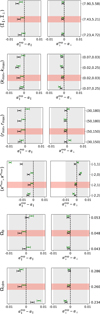 |
Fig. 3. Impact of the choice of fitting scales, fiducial cosmology, broadening Σ’s parameters and polynomial broadband order in the recovered values of the parameters α∥ and α⊥. Each point is the best-fit from the average of the 1000 EZmocks. The JS results are in green and GA in black. The grey shaded areas correspond to a 1% error and red shared areas indicate the fiducial choices of our analysis. |
Overall, the inferred value for the parameter α⊥ is the more robust than α∥ for both methods. Globally, GA and JS behave in the same way when varying the fitting configuration, proving that these are not caused by the new methodology. Best values and uncertainties are consistent between GA and JS. The systematic shifts for α∥ are smaller in JS, while no significant difference is seen for α⊥. The chosen baseline for the rest of the analysis is highlighted in red. The systematic errors may partially result from the covariance matrix that would require more realisations, but as they are much smaller than statistical errors budget for the real data (σα/α ∼ 2%), we can safely neglect these.
4.2. Fits on individual mocks
We now focus on the statistical properties of best-fit values and their uncertainties, based on fits of individual realisations of EZmocks. When fitting individual mocks, we fix (Σ∥,Σ⊥) to the best-fit values of the Joint analysis in the stack of 1000 measurements (see previous section), while letting all other parameters free. Table 3 summarises the parameters and flat priors used in these fits. The constraints on (α∥,α⊥) are then obtained by marginalizing over b and all other nuisance parameters.
Parameters used in the fits, with their flat priors.
For each method (FS, CS and JS) we remove results from nonconverging likelihoods (unsuccessful contour estimation) and extreme best-fit values at 5σ level (σ is defined as half of the range covered by the central 68% values). The best-fit values for which the estimated uncertainties touch the prior boundaries are removed as well. The remaining number of realisations referred as Ngood is given for each method in Table 4 and is consistent with the results of Gil-Marín et al. (2020) and Bautista et al. (2021).
Statistics on the fit of the 1000 EZmocks realisations.
To obtain GA results, we extract for each mock posterior profile the 1 sigma contour of the parameter space. We fit the likelihood contours corresponding to 68% C.L. with an ellipse, which we translate into a parameter covariance matrix Cmm, where m refers to either CS or FS. We scale the resulting covariance with the parameter m1 (see Table 2). We then construct the total covariance matrix 𝒞 from Eq. (13) obtained from the 1000 best-fit (α⊥, α∥), adjusting each time the coefficients (according to Eqs. (14) and (15)) to account for the observed errors of a given realisation. The corresponding correlation matrix before the individual adjustments is shown in Fig. 4. Using the combination method, we compute for each mock the consensus data vector xc and covariance Cc from Eqs. (11) and (12). Here we emphasize that the strong assumption of Gaussian elliptic contours for the parameters (α∥,α⊥) of every inference highly depends on the statistic of the considered tracer. The presence of non-Gaussian contours in our sample of mocks introduces biases in the total covariance matrix 𝒞 and each individual consensus data vector xc and covariance Cc. This is one of the limitations of the GA method that we can avoid with a JS fit.
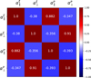 |
Fig. 4. Correlation coefficients between α∥ and α⊥ in CS and FS obtained from fits to the 1000 EZmock realisation. |
Figure 5 compares the distributions of α∥ (left) and α⊥ (right) and and their 1σ uncertainties as estimated by GA (top four panels) and JS (bottom four panels) versus the same quantities obtained from CS and FS fits. We see that the distributions are nicely correlated and scattered around the identity line (dashed). We find that the scatter (especially for errors) is less important between FS and JS than CS and JS. This would indicate that the Fourier space information has slightly more weight than the configuration space in the minimization of the likelihood. Moreover, while the GA errors are almost systematically inferior to the CS and FS ones, the JS errors are scattered on both sides of the dashed lines. Due to statistical fluctuations, JS analysis may result in looser constraints than FS or CS. We believe these fluctuations might origin from the finite number of mock realisations used to build the covariance matrix, though it is hard to test this hypothesis without a larger number of mocks.
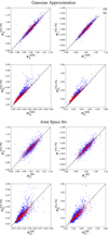 |
Fig. 5. Comparison between the distributions of the best-fit BAO parameters (α∥,α⊥) and their estimated errors obtained by fitting individual mock realisations. The four top (bottom) panels compare the CS (blue), FS (red) distributions with the GA (JS). The dashed lines represent a perfect correlation. |
Table 4 summarizes the statistical properties of (α∥,α⊥) for the different analyses, CS, FS, GA and JS, performed on 1000 EZmock realisations. For each parameter, we show six quantities: the average bias Δα = ⟨α − αexp⟩ with respect to the expected value (α⊥,exp = α∥,exp = 1), the standard deviation of best-fit values σ, the mean estimated error ⟨σi⟩, the mean asymmetry of the estimated error distribution  , the mean of the pull Zi = (αi−⟨αi⟩)/σi and its standard deviation. If errors are correctly estimated and follow a Gaussian distribution, we expect that σ = ⟨σi⟩, ⟨Z⟩=0 and σ(Zi)=1. Table 4 also shows the number Ngood of valid realisations after removing undetermined likelihoods, extreme values and errors, along with the mean value of the reduced chi-square
  .
.
Firstly, one can notice that the number of valid realisations (as defined above) for the JS analysis is larger than the one of the combined analysis GA. The GA method requires both FS and CS fits to converge, so the number of valid realisations for GA is necessarily the intersection of valid FS and CS realisations. By joining the information of both spaces, the JS fit is able to constrain the acoustic scale even on noisy mocks, where FS and CS separately fail. For each fitting procedure, we find the minimum reduced chi-square  , showing that the majority of the mocks are accurately modeled by our templates.
Secondly, we see good agreement between ⟨σi⟩ and σ for both parameters in all analyses. While the JS errors lies in between the CS and the FS errors for α∥, the combined results present in average smaller errors. Note that the standard deviation σ of the best-fit values are scaled with the appropriate correction factor  (see Table 2). A crucial issue with the GA method is m2 is ill-defined.
Overall, systematic shifts Δα for all methods are below half a per cent. The GA and JS methods yield reduced systematic shifts Δα than each individual space alone. While the shifts between GA and JS are the same for α⊥, the JS method yields slightly smaller shift for α∥ as also observed in the previous section.
If we assume that σ is a good estimate of the standard deviation of α, then the uncertainty of Δα should be  . In this case, all systematic shifts are smaller than 3σΔ except for α∥ in FS, which reaches a 3.5σΔ discrepancy. Shifts for GA are (−1.7, −1.8)σΔ for (α⊥, α∥) and (−1.5, −1.0)σΔ for JS fits. Note that our results are slightly different from those reported in Bautista et al. (2021) and Gil-Marín et al. (2020) due to a few differences in the analyses, such as how we decompose peak and smooth parts of the template, the number of polynomial terms, the values of non-linear damping terms.
Figure 6 displays the distributions of the pull Zi for α∥ and α⊥. For all four methods, the mean of the pull ⟨Zi⟩ is centered in zero to a few percent level, suggesting again that there are no systematic bias in the estimated α. Moreover the standard deviation of the pull σ(Zi) is smaller than one for both parameters in all analyses indicating a slight overestimation of the errors. This overestimation is more important for the parameter α∥, and in JS in general. As the standard deviation of the pulls are only a few percent away from unity, we do not attempt to correct these effects. If any overestimation of uncertainties is real, not correcting for it can be considered as an conservative approach. Yet, we see that for the parameter α∥ the overestimation of the errors reaches 10% in JS. While this seems to be significant, this result can be a consequence of the Gaussian assumption for the distribution of the parameters.
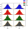 |
Fig. 6. Distributions of the pull Zi = (xi−⟨xi⟩)/σi for the parameters (α∥,α⊥) obtained obtained from the CS, FS, GA and JS analyses of the 1000 EZmocks sample. Orange curves describing a Gaussian distribution with zero mean and the standard deviation of the corresponding pull are shown for comparison. The dotted lines are centered on zero. |
To investigate the Gaussian nature of the distribution of the α’s parameters, we perform a D’Agostino-Pearson’s test (D’Agostino 1971; D’Agostino & Pearson 1973) on the sample of best-fit parameters using the SCIPY.STATS library5. The test combines the high-order statistical moments skewness and kurtosis to test the hypothesis that the two parameters are normally distributed. The statistical quantity K2 is constructed as a combination of the renormalized skewness and kurtosis such that K2 asymptotically follows a χ2 law with two degrees of freedom. When the skewness and kurtosis simultaneously deviate from 0 (Fisher kurtosis) K2 gets larger. The p-value for the K2 statistic is then to be compared with the risk a usually set to 5% for a Pearson test. As the a is the risk to reject the null hypothesis H0 while it is true, the p-value should be less than a to reject H0. Here the null hypothesis is that the α’s sample comes from a normal distribution. Table 5 shows the results of the Pearson tests on the α⊥, and α∥ distributions. Independently of the method, the Gaussian distribution hypothesis can be rejected for the parameter α∥ only, for which p/a < 1. This result indicates that for α∥, the smaller values of σ(Zi) observed in Table 4 might be partially induced by the non-Gaussianity of the α distributions and not simply by an overestimation of the uncertainties.
Results of D’Agostino and Pearson’s test of normality over the α’s distributions.
Figure 7 shows two dimensional confidence levels for a few realisations of mocks. Red contours are for FS results, blue for CS, green for JS and black for GA. The left panels are cases where the likelihoods can be approximated by a 2D Gaussian distribution while the right panels the opposite. In these examples, we can see how the JS fits are a better description for the non-Gaussian cases, where the final consensus are not necessarily Gaussian.
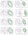 |
Fig. 7. Comparison between the different methods, using some EZmock realisations (mock tag above each plot), when the contours found in configuration or Fourier space are Gaussian (left) and non Gaussian (right). Red contours are for FS results, blue for CS, green for JS and black for GA. The expected value is the intersection of the dotted black lines, and the best fit values are described by a star for the JS and GA methods. We can see how the JS method yields better combined results that are not necessarily Gaussian. |
5. Application to eBOSS DR16 data
In this section, we apply our methodology to the eBOSS LRG sample, described in Sect. 2.1, letting free only α∥, α⊥, the linear density bias b and the broadband parameters.
Figure 8 shows the best-fit models for the power spectrum and correlation function multipoles, for three analyses: FS, CS and JS (note that we do not show a GA best-fit model as GA results are derived using the CS and FS best-fit). The residuals between in the bottom panels show excellent agreement between the JS model and the individual models for FS and CS, particularly over the BAO features. Furthermore, as the global amplitudes driven by the parameter b are sensibly the same, the small differences between the models arise mainly from the different broadbands. This is specially true for the correlation function as it is composed of fewer data bins.
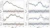 |
Fig. 8. Best monopole and quadrupole models for the CS, FS and JS analysis. The residues with respect to the measurements are standardized for each point by the errorbar. The grey shaded area correspond to a 1σ difference. |
Figure 9 shows the two dimensional 68 and 95% confidence levels for CS, FS, GA and JS. Once again we see an excellent agreement between the four analysis, with the JS giving slightly looser constraints. We also notice small differences in the inclination of the contours. The correlation coefficients for the CS, FS, GA and JS are respectively (−0.395, −0.404, −0.396, −0.445). Those values are consistent with the correlations found with 1000 EZmock realisations: (−0.380, −0.395, −0.383, −0.420). Note that this coefficient for the GA is highly dependent on the quality of the estimated correlation matrix of the parameters estimated from the EZmock sample and shown in Fig. 4. We find a higher correlation coefficient using the JS analysis, resulting in a thinner and steeper contours. This have for effect to increase the errors on the individual parameters without varying much the Figure-of-Merit (area of the contour, see Appendix D for a discussion on the FoM).
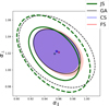 |
Fig. 9. Confidence contours of the parameters posterior distributions for the four analysis. For the CS and JS, the 1σ contours are filled in blue and red respectively. For the JS and GA we give the 1σ and 2σ contours for comparison in green and black. The best values are designated with a star. |
Table 6 summarises the results of the four different analysis. The reduced χ2 values are 1.28, 1.27 and 1.21 respectively for FS, CS and JS indicating relatively good adjustment to the data without over fitting from the broadband. In each case, the pvalue indicates a valid fit (if compared with a risk of 5%). The best fit values for the parameters (α⊥, α∥) are all in agreement according to their respective 1σ error bar. For both parameters, the JS analysis gives the larger uncertainty. Rescaling with the fiducial cosmology, we also derive the corresponding physical quantities DM/rd and DH/rd. Note that our best fit results do not exactly match the BAO constraints obtained in Bautista et al. (2021) and Gil-Marín et al. (2020), neither in configuration space nor in Fourier space, where the GA consensus gives DH/rd = 19.33 ± 0.53 and DM/rd = 17.86 ± 0.33 (third entry of Table 14 of Bautista et al. 2021). Those discrepancies arise from the slightly different non linear broadening parameters (Σ∥, Σ⊥) and a more flexible broadband polynomial expansion (imin, imax)=(−2, 1) to be compared to ( − 2, 0) for Bautista et al. (2021) and ( − 1, 1) for Gil-Marín et al. (2020).
Best-fit BAO parameters from the eBOSS DR16 LRG sample for different methods: configuration-space (CS), Fourier-space (FS), the Gaussian combination (GC) and our new joint-space fit (JS).
6. Conclusions
This work introduced a new BAO analysis of the DR16 eBOSS LRG sample, using Fourier and configuration-space information simultaneously. We compared the joint space (JS) analysis with the commonly used Gaussian approximation (GA) method, which combines results from the two spaces (Fourier and configuration) at the parameter level. The main advantage of the JS method is that it does not require any Gaussian assumption for the likelihood profiles. While the GA method is accurate only if the individual likelihoods to be combined are both Gaussian, yielding only Gaussian posterior distributions.
We assessed the systematic biases and errors of both methods by applying JS and GA to a set of 1000 EZMocks, which reproduce the eBOSS DR16 LRG sample properties. Compared to GA, JS provides a more accurate estimation of the acoustic scale by lowering the systematic shift of α∥ with respect to its expected value while GA has by construction a better precision (smaller error bars). Moreover, the JS offers a better control over variations of the analysis. Indeed the same mocks as the ones used to estimate the covariance are commonly used to perform systematic studies. Because of this, the standard deviation of any parameter should be rescaled with the correction factor m2 (see Table 2), which is not properly defined for the GA. One should note that because of larger size of the data vector, the JS methods requires a sufficiently large mock sample to estimate the covariance. However we found that the constraints are quite stable, and the number of mocks needed is not much larger than for a regular configuration or Fourier analysis.
We applied the different analysis to the eBOSS LRG sample and found consistent results (see Table 6). As expected from the statistical study the JS gives slightly looser constraints and a larger correlation coefficient. Despite providing looser constraints on cosmological parameters than the standard GA, we believe that JS is a more robust and reliable method for modelling the clustering signal by correctly accounting for the correlation between configuration and Fourier space and not relying on the Gaussianity of the parameter likelihoods.
One specific feature of the JS in a BAO analysis is that the broadband terms are independent between spaces. Hence, the JS introduces more nuisance parameters to be fitted simultaneously.
We are currently working on extending joint-space fits for measurements of the growth-rate of structures using information from the full shape of the power spectrum and correlation function. This work can also be extended to joint fits between pre and postreconstruction catalogs, as already performed in Fourier space by Gil-Marín (2022).
Acknowledgments
We would like to thank Hector Gil-Marín, Ashley Ross, Elena Sarpa, for useful discussions. The project leading to this publication has received funding from Excellence Initiative of Aix-Marseille University – A*MIDEX, a French “Investissements d’Avenir” program (AMX-20-CE-02 – DARKUNI).
References
- Alam, S., Ata, M., Bailey, S., et al. 2017, MNRAS, 470, 2617 [Google Scholar]
- Bautista, J. E., Vargas-Magaña, M., Dawson, K. S., et al. 2018, ApJ, 863, 110 [NASA ADS] [CrossRef] [Google Scholar]
- Bautista, J. E., Paviot, R., Vargas Magaña, M., et al. 2021, MNRAS, 500, 736 [Google Scholar]
- Beutler, F., Blake, C., Colless, M., et al. 2011, MNRAS, 416, 3017 [NASA ADS] [CrossRef] [Google Scholar]
- Bianchi, D., Gil-Marín, H., Ruggeri, R., & Percival, W. J. 2015, MNRAS, 453, L11 [NASA ADS] [CrossRef] [Google Scholar]
- Blanton, M. R., Bershady, M. A., Abolfathi, B., et al. 2017, AJ, 154, 28 [Google Scholar]
- Brout, D., Scolnic, D., Popovic, B., et al. 2022, ApJ, 938, 110 [NASA ADS] [CrossRef] [Google Scholar]
- Burden, A., Percival, W. J., & Howlett, C. 2015, MNRAS, 453, 456 [NASA ADS] [CrossRef] [Google Scholar]
- Carter, P., Beutler, F., Percival, W. J., et al. 2020, MNRAS, 494, 2076 [NASA ADS] [CrossRef] [Google Scholar]
- Chuang, C.-H., Kitaura, F.-S., Prada, F., Zhao, C., & Yepes, G. 2015, MNRAS, 446, 2621 [NASA ADS] [CrossRef] [Google Scholar]
- D’Agostino, R. B. 1971, Biometrika, 58, 341 [CrossRef] [Google Scholar]
- D’Agostino, R., & Pearson, E. S. 1973, Biometrika, 60, 613 [Google Scholar]
- Dawson, K. S., Schlegel, D. J., Ahn, C. P., et al. 2013, AJ, 145, 10 [Google Scholar]
- Dawson, K. S., Kneib, J.-P., Percival, W. J., et al. 2016, AJ, 151, 44 [Google Scholar]
- de Mattia, A., Ruhlmann-Kleider, V., Raichoor, A., et al. 2021, MNRAS, 501, 5616 [NASA ADS] [Google Scholar]
- DES Collaboration (Abbott, T., et al.) 2016, MNRAS, 460, 1270 [Google Scholar]
- DES Collaboration (Abbott, T. M. C., et al.) 2021, Phys. Rev. D, 105, 043512 [Google Scholar]
- Dodelson, S., & Schneider, M. D. 2013, Phys. Rev. D, 88, 063537 [Google Scholar]
- du Mas des Bourboux, H., Rich, J., Font-Ribera, A., et al. 2020, ApJ, 901, 153 [CrossRef] [Google Scholar]
- Eisenstein, D. J., Weinberg, D. H., Agol, E., et al. 2011, AJ, 142, 72 [Google Scholar]
- Gil-Marín, H. 2022, JCAP, 2022, 040 [CrossRef] [Google Scholar]
- Gil-Marín, H., Percival, W. J., Cuesta, A. J., et al. 2016, MNRAS, 460, 4210 [Google Scholar]
- Gil-Marín, H., Guy, J., Zarrouk, P., et al. 2018, MNRAS, 477, 1604 [Google Scholar]
- Gil-Marín, H., Bautista, J. E., Paviot, R., et al. 2020, MNRAS, 498, 2492 [Google Scholar]
- Grieb, J. N., Sánchez, A. G., Salazar-Albornoz, S., & Dalla-Vecchia, C. 2016, MNRAS, 457, 1577 [NASA ADS] [CrossRef] [Google Scholar]
- Gunn, J. E., Siegmund, W. A., Mannery, E. J., et al. 2006, AJ, 131, 2332 [NASA ADS] [CrossRef] [Google Scholar]
- Hamilton, A. J. S. 2000, MNRAS, 312, 257 [NASA ADS] [CrossRef] [Google Scholar]
- Hartlap, J., Simon, P., & Schneider, P. 2007, A&A, 464, 399 [NASA ADS] [CrossRef] [EDP Sciences] [Google Scholar]
- Hou, J., Sánchez, A. G., Ross, A. J., et al. 2021, MNRAS, 500, 1201 [Google Scholar]
- Howlett, C., Ross, A. J., Samushia, L., Percival, W. J., & Manera, M. 2015, MNRAS, 449, 848 [NASA ADS] [CrossRef] [Google Scholar]
- Kazin, E. A., Koda, J., Blake, C., et al. 2014, MNRAS, 441, 3524 [NASA ADS] [CrossRef] [Google Scholar]
- Kirkby, D., Margala, D., Slosar, A., et al. 2013, JCAP, 2013, 024 [CrossRef] [Google Scholar]
- Landy, S. D., & Szalay, A. S. 1993, ApJ, 412, 64 [Google Scholar]
- Lewis, A., Challinor, A., & Lasenby, A. 2000, ApJ, 538, 473 [Google Scholar]
- Neveux, R., Burtin, E., de Mattia, A., et al. 2020, MNRAS, 499, 210 [NASA ADS] [CrossRef] [Google Scholar]
- Percival, W. J., Ross, A. J., Sánchez, A. G., et al. 2014, MNRAS, 439, 2531 [NASA ADS] [CrossRef] [Google Scholar]
- Raichoor, A., de Mattia, A., Ross, A. J., et al. 2021, MNRAS, 500, 3254 [Google Scholar]
- Ross, A. J., Samushia, L., Howlett, C., et al. 2015a, MNRAS, 449, 835 [NASA ADS] [CrossRef] [Google Scholar]
- Ross, A. J., Percival, W. J., & Manera, M. 2015b, MNRAS, 451, 1331 [NASA ADS] [CrossRef] [Google Scholar]
- Ross, A. J., Beutler, F., Chuang, C.-H., et al. 2017, MNRAS, 464, 1168 [Google Scholar]
- Ross, A. J., Bautista, J., Tojeiro, R., et al. 2020, MNRAS, 498, 2354 [NASA ADS] [CrossRef] [Google Scholar]
- Sánchez, A. G., Grieb, J. N., Salazar-Albornoz, S., et al. 2017, MNRAS, 464, 1493 [CrossRef] [Google Scholar]
- Scoccimarro, R. 2015, Phys. Rev. D, 92, 083532 [NASA ADS] [CrossRef] [Google Scholar]
- Seo, H.-J., Beutler, F., Ross, A. J., & Saito, S. 2016, MNRAS, 460, 2453 [NASA ADS] [CrossRef] [Google Scholar]
- Smee, S. A., Gunn, J. E., Uomoto, A., et al. 2013, AJ, 146, 32 [Google Scholar]
- Tamone, A., Raichoor, A., Zhao, C., et al. 2020, MNRAS, 499, 5527 [Google Scholar]
- Taylor, A., Joachimi, B., & Kitching, T. 2013, MNRAS, 432, 1928 [Google Scholar]
- Yamamoto, K., Nakamichi, M., Kamino, A., Bassett, B. A., & Nishioka, H. 2006, PASJ, 58, 93 [Google Scholar]
- Zhao, C., Chuang, C.-H., Bautista, J., et al. 2021, MNRAS, 503, 1149 [CrossRef] [Google Scholar]
Appendix A: Fit with hexadecapole
Table A.1 shows the results for the fit of the averaged 1000 EZmocks, with and without using the hexadecapole. For every analysis the use of the additional information results in a slight increase of the systematic bias and of the errors bars. The looser constraints mainly arise from the larger size of the data vector when using hexadecapole. Indeed a larger amount of data bins results in an increase of the Whishart bound through the rescaling parameter m1 (especially for the JS analysis). Thus we decide not to use the hexadecapole information in this work.
Results for the fit of the 1000 EZmocks stack with and without using the hexadecapole information. For each parameter, we show the bias Δα ≡ (αi − αexp) and the estimated uncertainties σα.
Appendix B: Prereconstruction results
We perform fits on average correlations and individual mocks for the prereconstruction sample. Figure B.1 presents the impact of different parameters choice on the best fit values of α∥ and α⊥ for the GA (in black) and JS (in green) analysis. In every plot, a grey shaded area represents the 1 percent deviation from the expected value. Both analysis appears to be more dependant on the range of scales used (particularly in fourier space) as the small scales non linearities are not well modeled. However, without the reconstruction procedure that requires a fiducial cosmology, the dependence on Ωb and Ωcdm is reduced. The two analysis gives different results for the parameter α∥, the JS analysis tends to give a positive bias while the GA gives a negative.
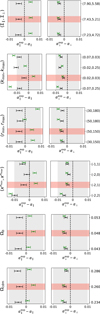 |
Fig. B.1. Impact of the choice of fitting scales, fiducial cosmology, broadening Σ’s parameters and polynomial broadband order in the recovered values of the parameters α∥ and α⊥. Each point is the best-fit from the average of the 1000 prereconstruction EZmocks. The JS method is in green and GA method is in black. The grey shaded areas correspond to a 1 percent error and red shared areas indicate the fiducial choices of our analysis. |
Figure B.2 shows the correlation matrix between the prereconstructed 2PCF and PS. The main differences between prereconstruction and postreconstruction covariance matrices are in the off-diagonal blocks within each space (either FS or CS), which are significantly reduced in postreconstruction. We construct the α’s parameters prereconstruction total covariance matrix obtained from the 1000 best-fit (α⊥, α∥). The corresponding correlation matrix before the individual adjustments is shown in Figure B.3. The reconstruction procedure enhances the correlations for a given parameter in two spaces, but reduces the correlations between the two parameters themselves (both in a given space and across spaces). Overall, the measurements depend on the signal-to-noise ratio of the BAO features, which are lower for prereconstruction data.
Table B.1 summarises the statistical properties of (α∥,α⊥) for the different analyses, CS, FS, GA and JS, performed on 1000 EZmock realisations. For each parameter, we show six quantities: the average bias Δα = ⟨α − αexp⟩ with respect to the expected value (α⊥,exp = α∥,exp = 1), the standard deviation of best-fit values σ, the mean estimated error ⟨σi⟩, the mean asymmetry of the estimated error distribution
Statistics on the fit of the 1000 EZmocks prereconstruction realisations. Ngood is the number of valid realisations after removing undefined contours and extreme values and errors. We show the mean value of the best-fit reduced  . For each parameter, we show the average bias Δα ≡ ⟨αi − αexp⟩, the standard deviation of best-fit values
  , the average of the per-mock estimated uncertainties ⟨σi⟩, the asymmetry of the estimated error distribution
  , where
  and
and  are the superior and inferior one sigma errors estimated from the likelihood profile, the average of the pull Zi ≡ (αi − ⟨αi⟩)/σi and its standard deviation σ(Zi).
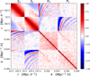 |
Fig. B.2. Correlation matrix of the correlation function ξℓ and power spectrum multipoles Pℓ estimated using the 1000 independent measurements of prereconstructed EZmocks. |
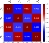 |
Fig. B.3. Correlation coefficients between α∥ and α⊥ in CS and FS obtained from fits to the prereconstructed 1000 EZmock realisation. |
 , the mean of the pull Zi = (αi−⟨αi⟩)/σi and its standard deviation. If errors are correctly estimated and follow a Gaussian distribution, we expect that σ = ⟨σi⟩, ⟨Z⟩=0 and σ(Zi)=1. For both parameters, the JS analysis presents larger systematic shifts Δα and larger errors than the GA. For the four analysis, σ(Zi) is larger than one, indicating an underestimation of the errors. This effect is more important for the GA. As our modelling is not well suited to describe the non linearities of the prereconstruction two point statistics, for every analysis the precision and accuracy are degraded. Here the JS method takes into account the correlations between two observables that are not well modeled in the first place. However, using an appropriate full shape modeling and removing the broadbands nuisance parameters, the CS and FS should be described by the exact same set of parameters. Hence the JS could improve the analysis.
Appendix C: Modelisation of the cross correlation pattern
We propose an analytical description of the cross correlations between the correlation function and power spectrum multipoles. The 2-point statistic between the fluctuation field in configuration and fourier space is
 (C.1)
(C.1)
while assuming gaussian fields, the cross covariance is given by
![Mathematical equation: $$ \begin{aligned} Co{ v}\left[P(\boldsymbol{k}),\xi (\boldsymbol{r})\right]&= \langle \delta _{ g}(\boldsymbol{k})\delta _{ g}(-\boldsymbol{k})\delta _{ g}(\boldsymbol{r})\delta _{ g}(-\boldsymbol{r}) \rangle \nonumber \\&=\langle \delta _{ g}(\boldsymbol{k})\delta _{ g}(\boldsymbol{r})\rangle \langle \delta _{ g}(-\boldsymbol{k})\delta _{ g}(-\boldsymbol{r}) \rangle +\\&\quad \langle \delta _{ g}(\boldsymbol{k})\delta _{ g}(-\boldsymbol{r})\rangle \langle \delta _{ g}(-\boldsymbol{k})\delta _{ g}(\boldsymbol{r}) \rangle \nonumber \\&= 2\cos (2\boldsymbol{k} \cdot \boldsymbol{r})|P(\boldsymbol{k})|^2.\nonumber \end{aligned} $$](/articles/aa/full_html/2022/11/aa44100-22/aa44100-22-eq61.gif) (C.2)
(C.2)
Then, including the shot noise contribution PN and the volume rescaling, the cross covariance between the multipoles Pl(k) and ξl′(r) can be written
![Mathematical equation: $$ \begin{aligned} Co{ v}&\left[P_l(k),\xi _{l^\prime }(r)\right] = \frac{2l+1}{2}\frac{2l^\prime +1}{2}\frac{1}{Vs}\int _{-1}^{1}d\mu _k L_l(\mu _k) |P(k,\mu _k)+P_N|^2 \nonumber \\&\times \int _{-1}^{1}d\mu _r L_l(\mu _r) 2\cos \left(2rk\mu _k\mu _r+2kr\sqrt{1-\mu _k^2}\sqrt{1-\mu _r^2}\right). \end{aligned} $$](/articles/aa/full_html/2022/11/aa44100-22/aa44100-22-eq62.gif) (C.3)
(C.3)
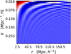 |
Fig. C.1. Analytical modeling of the cross correlations between the correlation function and the power spectrum monopoles for a given range of scales. We do not display the colorbar as we set the shot noise to zero and the volume of the survey to one. |
Figure C.1 shows the modeling of the cross covariance features using Eq C.2 for a given range of scales. We find this description satisfying as we only aim for a physical understanding of these patterns, and use the full mocks sample to estimate the covariance. A more reliable modeling would require bin averaged integral as performed in Grieb et al. (2016).
Appendix D: Mock dependant constraints
We tested the robustness of the different analysis against the number of available mock realisations. We fit the averaged stack of mocks for different values of Nmocks used to estimate the sample covariance matrix.
Figure D.1 shows the figure of merit defined as  with Cθ the covariance matrix of the inferred parameters, and the quadratic shift from the expected parameters
  for different Nmock. As expected we find that, due to the Whishart bound, the JS precision highly decreases when the number of mocks get small, typically the Fom drops when Nmock < 4Nbins. However the JS constraint is compatible with the GA at 1σ, and appears to be robust as the Fom does not decrease very much in the range 1000-600 Nmock. While the GA analysis introduces an additional dependence on Nmock through the covariance Cc defined in Eq 11 (which has to be calculated for each point using the set of best fit parameters found with the appropriated sample covariance), the Fom is only decreased by a few percent when using 100 realisations.
We find that for the JS the quadratic shift from the expected parameters monotonically decreases as the amount of mocks increases. For a large enough amount of realisations, the JS gives the smaller systematic bias.
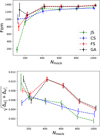 |
Fig. D.1. Figure of merit (Fom) and quadratic shift from the expected parameters resulting from the fit of the stack of EZmocks for different Nmock used to estimated the sample covariance. Errors for the α’s are scaled with |

All Tables
Results of D’Agostino and Pearson’s test of normality over the α’s distributions.
Best-fit BAO parameters from the eBOSS DR16 LRG sample for different methods: configuration-space (CS), Fourier-space (FS), the Gaussian combination (GC) and our new joint-space fit (JS).
Results for the fit of the 1000 EZmocks stack with and without using the hexadecapole information. For each parameter, we show the bias Δα ≡ (αi − αexp) and the estimated uncertainties σα.
Statistics on the fit of the 1000 EZmocks prereconstruction realisations. Ngood is the number of valid realisations after removing undefined contours and extreme values and errors. We show the mean value of the best-fit reduced . For each parameter, we show the average bias Δα ≡ ⟨αi − αexp⟩, the standard deviation of best-fit values , the average of the per-mock estimated uncertainties ⟨σi⟩, the asymmetry of the estimated error distribution , where and are the superior and inferior one sigma errors estimated from the likelihood profile, the average of the pull Zi ≡ (αi − ⟨αi⟩)/σi and its standard deviation σ(Zi).
All Figures
|
Fig. 1. Correlation matrix of the correlation function ξℓ and power spectrum multipoles Pℓ estimated using the 1000 independent measurements of EZmocks. |
| In the text | |
|
Fig. 2. Precision matrix of the correlation function ξℓ and power spectrum multipoles Pℓ. Top panel: normalized estimated precision matrix |
| In the text | |
|
Fig. 3. Impact of the choice of fitting scales, fiducial cosmology, broadening Σ’s parameters and polynomial broadband order in the recovered values of the parameters α∥ and α⊥. Each point is the best-fit from the average of the 1000 EZmocks. The JS results are in green and GA in black. The grey shaded areas correspond to a 1% error and red shared areas indicate the fiducial choices of our analysis. |
| In the text | |
|
Fig. 4. Correlation coefficients between α∥ and α⊥ in CS and FS obtained from fits to the 1000 EZmock realisation. |
| In the text | |
|
Fig. 5. Comparison between the distributions of the best-fit BAO parameters (α∥,α⊥) and their estimated errors obtained by fitting individual mock realisations. The four top (bottom) panels compare the CS (blue), FS (red) distributions with the GA (JS). The dashed lines represent a perfect correlation. |
| In the text | |
|
Fig. 6. Distributions of the pull Zi = (xi−⟨xi⟩)/σi for the parameters (α∥,α⊥) obtained obtained from the CS, FS, GA and JS analyses of the 1000 EZmocks sample. Orange curves describing a Gaussian distribution with zero mean and the standard deviation of the corresponding pull are shown for comparison. The dotted lines are centered on zero. |
| In the text | |
|
Fig. 7. Comparison between the different methods, using some EZmock realisations (mock tag above each plot), when the contours found in configuration or Fourier space are Gaussian (left) and non Gaussian (right). Red contours are for FS results, blue for CS, green for JS and black for GA. The expected value is the intersection of the dotted black lines, and the best fit values are described by a star for the JS and GA methods. We can see how the JS method yields better combined results that are not necessarily Gaussian. |
| In the text | |
|
Fig. 8. Best monopole and quadrupole models for the CS, FS and JS analysis. The residues with respect to the measurements are standardized for each point by the errorbar. The grey shaded area correspond to a 1σ difference. |
| In the text | |
|
Fig. 9. Confidence contours of the parameters posterior distributions for the four analysis. For the CS and JS, the 1σ contours are filled in blue and red respectively. For the JS and GA we give the 1σ and 2σ contours for comparison in green and black. The best values are designated with a star. |
| In the text | |
|
Fig. B.1. Impact of the choice of fitting scales, fiducial cosmology, broadening Σ’s parameters and polynomial broadband order in the recovered values of the parameters α∥ and α⊥. Each point is the best-fit from the average of the 1000 prereconstruction EZmocks. The JS method is in green and GA method is in black. The grey shaded areas correspond to a 1 percent error and red shared areas indicate the fiducial choices of our analysis. |
| In the text | |
|
Fig. B.2. Correlation matrix of the correlation function ξℓ and power spectrum multipoles Pℓ estimated using the 1000 independent measurements of prereconstructed EZmocks. |
| In the text | |
|
Fig. B.3. Correlation coefficients between α∥ and α⊥ in CS and FS obtained from fits to the prereconstructed 1000 EZmock realisation. |
| In the text | |
|
Fig. C.1. Analytical modeling of the cross correlations between the correlation function and the power spectrum monopoles for a given range of scales. We do not display the colorbar as we set the shot noise to zero and the volume of the survey to one. |
| In the text | |
|
Fig. D.1. Figure of merit (Fom) and quadratic shift from the expected parameters resulting from the fit of the stack of EZmocks for different Nmock used to estimated the sample covariance. Errors for the α’s are scaled with |
| In the text | |
Current usage metrics show cumulative count of Article Views (full-text article views including HTML views, PDF and ePub downloads, according to the available data) and Abstracts Views on Vision4Press platform.
Data correspond to usage on the plateform after 2015. The current usage metrics is available 48-96 hours after online publication and is updated daily on week days.
Initial download of the metrics may take a while.