© J.-B. Delisle and D. Ségransan 2022

1 Introduction

The Gaia mission started its nominal operations in 2014 to monitor the positions of a billion stars. The amount of data generated by the spacecraft is massive and their calibration and analysis represent a vast processing challenge. In this context, the computing time dedicated to the analysis of each target is necessarily limited and efficient analysis methods have to be developed. In this article, we present efficient analytical methods for detecting and characterizing companions (planets, brown dwarfs, or stars) in astrometric time series as well as via a combination of astrometric and radial velocity time series. This study is part of an effort to improve the Gaia exoplanet detection pipeline and, more specifically, the MIKS-GA¹ algorithms (Holl et al. 2022). The methods presented here have been partially integrated in MIKS-GA for the third Gaia data release (DR3).

The least-squares or Lomb-Scargle (LS) periodogram (Lomb 1976; Scargle 1982) and subsequent generalizations (e.g., Ferraz-Mello 1981; Zechmeister & Kürster 2009) are powerful tools in the search for periodicities in uneven time series and widely used in many branches of astronomy. In the context of two-dimensional (2D) astrometry (i.e., when both sky coordinates are measured at once, with a similar level of precision), the LS periodogram has also been used to search for periodicities on each coordinate independently (e.g., Black & Scargle 1982) or jointly (e.g., Catanzarite et al. 2006). More sophisticated periodograms have also been developed in the case of 2D astrometry, for instance, the phase distance correlation periodogram (Zucker 2019). However, to our knowledge, these approaches have not been extended to the case of scanning space astrometric missions, such as Hipparcos and Gaia. Here, we propose a general linear periodogram framework to efficiently locate the periods of candidate companions among scanning space astrometric time series alone and among astrometric and radial velocity time series combined. We additionally derive an analytical false alarm probability (FAP) criterion to assess the significance of the candidates. This periodogram and FAP framework builds on the previous works of Baluev (2008) and Delisle et al. (2020a), which were primarily focused on the analysis of radial velocity time series.

Once a companion is detected and its period is known, the next step is to determine the complete set of parameters describing its orbit. This is usually achieved using numerical methods, such as least-squares minimization (or likelihood maximization) algorithms, or Markov chain Monte-Carlo. However these numerical methods can be expensive in terms of computing time, especially if the initialization of the parameters is far from the solution. Here, we propose an analytical method that can efficiently determine approximate orbital elements, which may be used as the initial conditions for numerical methods. it relies on the Fourier decomposition of the time series. indeed, for an eccentric orbit, the signature of the companion has some power at the orbital period, but also at the harmonics of the orbital period. In particular, the amplitude at the first harmonics is approximately proportional to the eccentricity. We used such properties to derive all the orbital parameters from a linear least-square fit with sinusoids at the orbital period and its first harmonics. Similar methods have been developed in the context of astrometry with the cancelled space interferometry mission (SIM), (Konacki et al. 2002) and radial velocities (Correia 2008; Delisle et al. 2016). In this work, we extend the method proposed in Delisle et al. (2016) to the case of scanning space astrometry as well as to the case where astrometry and radial velocities are combined.

This article is organized as follows. In Sect. 2, we present the scanning space astrometric method and the expected astrometric signature of an unseen companion orbiting a star. Then, we define in Sect. 3 a general linear periodogram for an astrometric time series and its combination with radial velocities and we derive analytical approximations of the corresponding FAp. We obtain in Sect. 4 analytical formulas to derive an approximation of all the orbital parameters once the period is known. We illustrate our methods in Sect. 5 to reanalyze the astrometric and radial velocity time series of three stars known to host companions. While our methods have been developed in view of analyzing Gaia data, we had to fall back to illustrating them on the basis of Hipparcos data, since Gaia astrometric time series will not be publicly available before DR4. Finally, we discuss in Sect. 6 the possible uses of these methods.

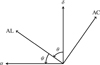Fig. 1 Scan angle convention for Gaia (θ) and Hipparcos (ψ).

2 Scanning space astrometry and Keplerian motion

2.1 Coordinates and scan-angle

Scanning space astrometric missions such as Hipparcos or Gaia do not directly measure the instantaneous declination (δ) and right-ascension (α) of a star in the ICRS frame. They instead measure the abscissa, s_AL, of the star along a scan direction with great precision, while the perpendicular coordinate, s_AC, is determined with a much lower precision. The measured coordinates (s_AL, s_AC) depend on the scanning direction which is represented with a different convention between Gaia and Hipparcos (see Fig. 1). The Gaia scan angle θ is the angle between the north (increasing δ) and the along-scan direction (increasing s_AL), while the Hipparcos scan angle ψ is the angle between the along-scan direction and the East (increasing α). We thus have:

$$\begin{array}{lll}\psi \hfill & =\hfill & \frac{\pi }{2}-\theta ,\hfill \\ s_{\text{AL}}\hfill & =\hfill & \delta \cos \theta +{\alpha }^{*}\sin \theta +\varpi {\text{Π}}_{\text{AL}}\hfill \\ \hfill & =\hfill & \delta \cos \psi +{\alpha }^{*}\sin \psi +\varpi {\text{Π}}_{\text{AL}},\hfill \\ s_{\text{AC}}\hfill & =\hfill & \delta \sin \theta -{\alpha }^{*}\cos \theta +\varpi {\text{Π}}_{\text{AC}}\hfill \\ \hfill & =\hfill & \delta \cos \psi -{\alpha }^{*}\sin \psi +\varpi {\text{Π}}_{\text{AC}},\hfill \end{array}$$(1)

where α* = α cos δ is the modified right-ascension, ϖ is the parallax, and ∏_AL, ∏_AC are the parallax factors. Across scan observations can actually be treated the same way as along scan observations by defining θ′ = θ − π/2 and ψ′ = ψ + π/2. in the following, we assume that all the observations (Gaia or Hipparcos, along or across scan) are converted to follow the Gaia along-scan convention

$$s=\delta \cos \theta +{\alpha }^{*}\sin \theta +\varpi \text{Π}.$$(2)

The instantaneous coordinates of the star (δ, α*) evolve due to the proper motion of the system barycenter and to potential companions. The proper motion can be expressed as a polynomial expansion over time, so the coordinates follow

$$\begin{array}{lll}\delta \left(t\right)\hfill & =\hfill & {\delta }_0+{\displaystyle \sum _{k=1}^{k_{\max }}{\mu }_{\delta }^{\left(k\right)}{t}^k+{\delta }_K\left(t\right),}\hfill \\ {\alpha }^{*}\left(t\right)\hfill & =\hfill & {\alpha }_0^{*}+{\displaystyle \sum _{k=1}^{k_{\max }}{\mu }_{\alpha *}^{\left(k\right)}{t}^k+{\alpha }_K\left(t\right),}\hfill \end{array}$$(3)

where $\left({\delta }_0,{\alpha }_0^{*}\right)$ is the position of the system barycenter at the reference epoch (t = 0), k_max is the degree of the expansion of the proper motion, ${\mu }_{\delta }^{\left(k\right)},{\mu }_{\alpha *}^{\left(k\right)}$ are the coefficients of this expansion, and (δ_K, α_K) is the Keplerian part of the signal (due to companions). in most cases, only a linear proper motion is accounted for (k_max = 1), and we simplify the notations as ${\mu }_{\delta }={\mu }_{\delta }^{\left(1\right)},{\mu }_{\alpha *}^{\left(k\right)}={\mu }_{\alpha *}^{\left(1\right)}$

2.2 Keplerian astrometric signal

Here, we consider a star that is orbited by a single companion, assuming that the orbit is Keplerian. This Keplerian motion is given by

$$\begin{array}{lll}{\delta }_K\hfill & =\hfill & Ax+Fy,\hfill \\ {\alpha }_K\hfill & =\hfill & Bx+Gy,\hfill \end{array}$$(4)

where

$$\begin{array}{lll}x\hfill & =\hfill & \cos E-e,\hfill \\ y\hfill & =\hfill & \sqrt{1-e^2}\sin E,\hfill \end{array}$$(5)

with e as the eccentricity, E the eccentric anomaly, and A, B, F, G the Thiele-Innes coefficients

$$\begin{array}{lll}A\hfill & =\hfill & a_s\left(\cos \omega \cos \text{Ω}-sin\omega sin\text{Ω}\cos i\right),\hfill \\ B\hfill & =\hfill & a_s\left(\cos \omega sin\text{Ω}+sin\omega \cos \text{Ω}\cos i\right),\hfill \\ F\hfill & =\hfill & a_s\left(-\sin \omega \cos \text{Ω}-\cos \omega sin\text{Ω}\cos i\right),\hfill \\ G\hfill & =\hfill & a_s\left(-\sin \omega \sin \text{Ω}-\cos \omega \cos \text{Ω}\cos i\right),\hfill \end{array}$$(6)

where ω, Ω, and i are the argument of periastron, longitude of ascending node, and inclination of the orbit, respectively, and a_s is the semi-major axis of the orbit of the star around the center of mass of the system, expressed in mas. The eccentric anomaly is implicitly expressed as a function of time through the Kepler equation

$$E-e\sin E=M=M_0+2\pi \frac{t}{P},$$(7)

where M is the mean anomaly, M₀ is the mean anomaly at the reference epoch, and P is the orbital period.

2.3 Fourier decomposition of a Keplerian astrometric signal

The Keplerian part of the astrometric signal is P-periodic and can be decomposed as a discrete Fourier series

$$\begin{array}{lll}{\delta }_K\hfill & =\hfill & {\displaystyle \sum _{k\in \mathbb{Z}}{d}_k{\text{e}}^{\text{i}knt}},\hfill \\ {\alpha }_K\hfill & =\hfill & {\displaystyle \sum _{k\in \mathbb{Z}}{a}_k{\text{e}}^{\text{i}knt}},\hfill \end{array}$$(8)

with n = 2π/P as the planet mean-motion. We introduce the complex coordinate,

$$\zeta =x+iy=\cos E-e+\text{i}\sqrt{1-e^2}\text{sin\hspace{0.17em}}E,$$(9)

and the complex coefficients,

$$\begin{array}{lll}{P}_{\delta }{\text{e}}^{i{\varphi }_{\delta }}\hfill & =\hfill & \frac{A-\text{i}F}{2},\hfill \\ P_{\alpha }{\text{e}}^{i{\varphi }_{\alpha }}\hfill & =\hfill & \frac{B-\text{i}G}{2},\hfill \end{array}$$(10)

such that

$$\begin{array}{lll}{\delta }_K\hfill & =\hfill & P_{\delta }\left({\text{e}}^{\text{i}{\varphi }_{\delta }}\zeta +{\text{e}}^{-\text{i}{\varphi }_{\delta }}\overline{\zeta }\right),\hfill \\ {\alpha }_K\hfill & =\hfill & P_{\alpha }\left({\text{e}}^{\text{i}{\varphi }_{\alpha }}\zeta +{\text{e}}^{-\text{i}{\varphi }_{\alpha }}\overline{\zeta }\right).\hfill \end{array}$$(11)

We then write the Fourier decomposition of ζ in the following form:

$$\zeta \left(t\right)={\displaystyle \sum _{k\in \mathbb{Z}}{\zeta }_k{\text{e}}^{\text{i}kM}}={\displaystyle \sum _{k\in \mathbb{Z}}{\zeta }_k{\text{e}}^{\text{i}k{M}_0}{\text{e}}^{\text{i}knt}},$$(12)

where

$${\zeta }_k=\frac{1}{2\pi }{\displaystyle {\int }_0^{2\pi }\zeta {\text{e}}^{-\text{i}kM}\text{d}M}$$(13)

are functions of the eccentricity only. The coefficients d_k and a_k are then easily expressed as functions of the coefficients ζ_k

$$\begin{array}{lll}{d}_k\hfill & =\hfill & P_{\delta }{\text{e}}^{\text{i}k{M}_0}\left({\text{e}}^{i{\varphi }_{\delta }}{\zeta }_k+{\text{e}}^{-i{\varphi }_{\delta }}{\zeta }_{-k}\right),\hfill \\ a_k\hfill & =\hfill & P_{\alpha }{\text{e}}^{\text{i}k{M}_0}\left({\text{e}}^{i{\varphi }_{\alpha }}{\zeta }_k+{\text{e}}^{-i{\varphi }_{\alpha }}{\zeta }_{-k}\right).\hfill \end{array}$$(14)

The coefficients ζ_k can be computed numerically (see Appendix A). They can also be computed analytically as power series of the eccentricity. We go on to rewrite Eq. (13) as an integral over the eccentric anomaly, E,

$$\begin{array}{lll}{\zeta }_k\hfill & =\hfill & \frac{1}{2\pi }{\displaystyle {\int }_0^{2\pi }\left(\cos E-e+\text{i}\sqrt{1-e^2}\sin E\right)}\hfill \\ \hfill & \hfill & \times {\text{e}}^{-\text{i}k\left(E-e\sin E\right)}\left(1-e\cos E\right)\text{d}E.\hfill \end{array}$$(15)

This expression can then straightforwardly be developed in power series of the eccentricity and integrated over E. We obtain for the first terms:

$$\begin{array}{lll}{\zeta }_0\hfill & =\hfill & -\frac{3}{2}e,\hfill \\ {\zeta }_1\hfill & =\hfill & 1-\frac{1}{2}{e}^2+O\left(e^4\right),\hfill \\ {\zeta }_{-1}\hfill & =\hfill & \frac{1}{8}{e}^2+O\left(e^4\right),\hfill \\ {\zeta }_2\hfill & =\hfill & \frac{1}{2}e-\frac{3}{8}{e}^3+O\left(e^5\right),\hfill \\ {\zeta }_{-2}\hfill & =\hfill & \frac{1}{24}{e}^3+O\left(e^5\right).\hfill \end{array}$$(16)

At low eccentricity, the leading Fourier coefficients of δ and α are found at the orbital period. The amplitude of the first harmonics (half the orbital period) terms is proportional to the eccentricity. Higher order harmonics have a much lower amplitude (higher powers of the eccentricity). In the following, we aim to detect the presence of a companion using a linear periodogram approach where we approximate the Keplerian signal with the fundamental frequency only. Then, once the companion is detected and its orbital period is known, we estimate the remaining parameters by approximating the Keplerian signal using the fundamental and the first harmonics. These two approximations remain valid for low to moderate eccentricity. In order to assess the domain of validity of this approach, we estimated the fraction of the signal power that lies in the fundamental and in the first harmonics. We show, in Fig. 2, these power fractions as a function of the eccentricity. As a comparison, we also provide the same fractions in the case of a radial velocity Keplerian signal. The details of these derivations are presented in Appendix A. As expected, we see in Fig. 2 that at low eccentricity, the power of the signal is concentrated in the fundamental frequency both for a radial velocity signal and an astrometric signal. However, the behavior of both kinds of signal differs at higher eccentricity. For the radial velocities, the power fraction in the fundamental drops to zero when the eccentricity reaches 1. Therefore, for a radial velocity signal, the linear periodogram approach (with a single frequency) has a significant loss of sensitivity for high eccentricity signals (see also Baluev 2015). To circumvent this issue, more complex periodogram definitions have been proposed in the literature (e.g., Baluev 2013, 2015; Zucker 2018). In the case of astrometry, the power fraction in the fundamental also decreases with eccentricity, but it always remains above about 80 %. Therefore, the linear periodogram approach remains fairly sensitive even for highly eccentric orbits, and a more complex periodogram approach would probably be less beneficial than in the radial velocity case.

While a high power fraction in the fundamental improves the detection sensitivity of the linear periodogram, it also reduces the ability to characterize the companion’s eccentricity and argument of periastron. Indeed, the fundamental frequency alone does not contain sufficient information to derive these parameters. Therefore, one can only derive the eccentricity and argument of periastron with good precision for a signal that has significant power in the harmonics. This applies in particular to our analytical method (Sect. 4) but, more generally, independently of the method, we expect the eccentricity and argument of periastron to be characterized with less precision using astrometry than using radial velocities, for a similar signal to noise ratio (S/N).

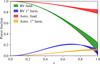Fig. 2 Fraction of the signal power in the fundamental and in the first harmonics for a radial velocity time series and an astrometric time series.

3 Periodogram and false alarm probability

3.1 General linear periodogram

Here, we adopt a periodogram approach to detect the signature of a companion and estimate its orbital period. Following Baluev (2008); Delisle et al. (2020a), we define a general linear periodogram by comparing the χ² of the residuals of a linear base model, H, with p parameters and enlarged linear model, K, of p + d parameters, further parameterized by the angular frequency, v. The linear base model, H, follows:

$$\begin{array}{cc}H:& m_H\left({\beta }_H\right)={\phi }_H{\beta }_H,\end{array}$$(17)

where β_H is the vector of size p of the model parameters, φ_H is a n × p matrix, and n is the number of points in the time series. Typically, this base model includes five linear parameters, including the position, the proper motion, and the parallax (see Eqs. (2), (3)):

$$\begin{array}{lll}{\beta }_H\hfill & =\hfill & \left({\delta }_0,{\alpha }_0^{*},{\mu }_{\delta },{\mu }_{\alpha },\pi \right),\hfill \\ {\phi }_H\hfill & =\hfill & \left(\begin{array}{ccccc}\cos {\theta }_1& \sin {\theta }_1& t_1\cos {\theta }_1& t_1\sin {\theta }_1& {\text{Π}}_1\\ \cos {\theta }_2& \sin {\theta }_2& t_2\cos {\theta }_2& t_2\sin {\theta }_2& {\text{Π}}_2\\ ⋮& ⋮& ⋮& ⋮& ⋮\\ \cos {\theta }_n& \sin {\theta }_n& t_n\cos {\theta }_n& t_n\sin {\theta }_n& {\text{Π}}_n\end{array}\right),\hfill \end{array}$$(18)

but any additional linear parameters might be included. For instance, a quadratic proper motion can be accounted for by adding the columns t² cos θ, t² sin θ in φ_H.

The enlarged model K(v) follows

$$\begin{array}{cc}K\left(v\right):& m_K\left(v,{\beta }_K\right)\end{array}={\phi }_K\left(v\right){\beta }_K,$$(19)

where β_K = (β_H,β) is the vector of the p + d linear parameters, and φ_K(v) is the n × (p + d) matrix whose p first columns are the columns of φ_H, and whose d last columns are functions of the angular frequency, v.

In the case of radial velocities (see Baluev 2008; Delisle et al. 2020a), we would typically have d = 2, with the additional columns of cos vt and sin vt, to account for any possible phase of the potential companion. This definition implicitly assumes that the signature of the companion is dominated by the fundamental frequency (see Sect. 2.3). In the astrometric case, the same approximation is achieved with the d = 4 additional columns: cos θ cos vt, sin θ cos vt, cos θ sin vt, and sin θ sin vt. These four terms allow us to account for any possible phase and for the projection of the orbit over both axes (see Eqs. (2), (3)). Thus, we typically use

$$\begin{array}{lll}{\beta }_K\hfill & =\hfill & \left({\beta }_H,{\beta }_{\delta ,c},{\beta }_{\alpha ,c},{\beta }_{\delta ,s},{\beta }_{\alpha ,s}\right),\hfill \\ {\phi }_K\left(v\right)\hfill & =\hfill & \left({\phi }_H,\cos \theta \cos vt,\sin \theta \cos vt,\cos \theta \sin vt,\sin \theta \sin vt\right),\hfill \end{array}$$(20)

where β_K is the vector of the p + 4 parameters, and φ_K is the (n × (p + 4)) matrix obtained by horizontal concatenation of φ_H and the four additional columns.

We denote by ${\chi }_H^2$ and ${\chi }_K^2$ the χ² of the residuals after a linear least squares fit with a covariance matrix C of the models H and K(v), respectively:

$$\begin{array}{lll}{\chi }_H^2\hfill & =\hfill & {\left(s-{\phi }_H{\beta }_H\right)}^T{C}^{-1}\left(s-{\phi }_H{\beta }_H\right),\hfill \\ {\chi }_K^2\left(v\right)\hfill & =\hfill & {\left(s-{\phi }_K{\beta }_K\left(v\right){\beta }_K\right)}^T{C}^{-1}\left(s-{\phi }_K\left(v\right){\beta }_K\right).\hfill \end{array}$$(21)

The covariance matrix, C, may account for all sources of correlated and uncorrelated noise, and in particular the instrument systematics.

In the general case, the periodogram is a function $f\left({\chi }_H^2,{\chi }_K^2\left(v\right)\right)$. A general linear periodogram z is thus defined by the models, H and K(v), and the function f. For instance, the widespread GLS periodogram (see Ferraz-Mello 1981; Zechmeister & Kürster 2009) is defined as

$$z_{\text{GLS}}\left(v\right)=\frac{{\chi }_H^2-{\chi }_K^2\left(v\right)}{{\chi }_H^2}.$$(22)

Baluev (2008) proposed four alternative definitions of the periodogram. In the following, we focus on the GLS periodogram since it is more widely used, but similar derivations can be found in Appendix B for these alternative definitions.

3.2 False alarm probability

Once the periodogram is computed, it is useful to compute the p-value of the highest peak (FAP), defined as:

$${\text{FAP}}_{\max }\left(Z,v_{\max }\right)=\mathrm{Pr}\left\{\underset{v<v_{\max }}{\max }z\left(v\right)\ge Z|H\right\},$$(23)

where Z is the value of the maximum peak of the periodogram computed on the data. In this section, we provide analytical approximations of the FAP for the GLS periodogram of Eq. (22). Similar approximations for the alternative periodogram definitions and their precise derivation is provided in Appendix B.

The model H is defined as in Eq. (17), where the n × p matrix φ_H is user-defined, and the model K is defined as in Eq. (20). The periodogram is computed in the range of frequencies ]0, v_max] (i.e., 0 excluded and v_max included). The FAP is approximated by (see Baluev 2008):

$${\text{FAP}}_{\max }\left(Z,v_{\max }\right)\approx 1-\left(1-{\text{FAP}}_{\text{single}}\left(Z\right)\right){\text{e}}^{-\tau \left(Z,v_{\max }\right)},$$(24)

where analytical expressions for FAP_single and τ(Z, v_max) are given in Table 1 (d = 4). These expressions depend on the rescaled frequency bandwidth, W, defined as

$$W=\frac{v_{\max }}{2\pi }{T}_{\text{eff}},$$(25)

where T_eff is the effective time series length. We provide in Appendix B analytical estimates of T_eff in the general case of correlated noise. In the simplest case of white noise, that is, for a diagonal covariance matrix C = diag(σ²), the effective time series length can be approximated by

$$T_{\text{eff}}\approx \sqrt{4\pi \left(\overline{t^2}-{\overline{t}}^2\right)},$$(26)

where $\overline{t}$ and $\overline{t^2}$ are weighted means with weights ${\sigma }_i^2\text{/}{\displaystyle {\sum }_j{\sigma }_j^2}$. This expression is proportional to the weighted standard deviation of the measurement times.

The FAP estimate that we obtain here rely on the correct estimation of the power, Z, of the highest peak in the considered range of angular frequency ]0, v_max]. When computing the periodogram, we should thus sample v with a sufficiently small step size to determine Z with a good precision. Moreover, it is also important for the following steps to correctly identify the period of the highest peak, which also requires for the periodogram to be correctly sampled. The width of periodogram peaks is typically 2π/T_eff (in angular frequency). Each peak should be sampled with a sufficient number of points to obtain a good estimation of the peak height. A standard procedure in the literature is to sample the angular frequency linearly with a step size of 2π/n_oT where T is the total time span of the observations (which is a proxy for T_eff), and n_o > 10 is the oversampling factor. The maximum angular frequency v_max, or equivalently the minimum period P_min, is user-defined. By increasing the size of the frequency range, we increase the probability of obtaining a higher peak by chance (null hypothesis), which is why the FAP estimate takes into account the maximum frequency, v_max, through the rescaled frequency bandwidth, W.

3.3 Combining astrometric and radial velocity time series

We now consider the case where both astrometric and radial velocity time series are available for a source. We extend to this case the periodogram and analytical FAP approach described above. In the following, we assume that the calendars of astrometric and radial velocity observations are independent and that the noise affecting both time series is independent.

The general linear periodogram framework described above is compatible with heterogeneous time series (such as astrometry and radial velocities). We define the full dataset as a concatenation of the astrometric and radial velocity datasets:

$$\begin{array}{lll}t\hfill & =\hfill & \left(t_{\text{a}},t_{\text{v}}\right)\hfill \\ y\hfill & =\hfill & \left(s,v\right),\hfill \end{array}$$(27)

where t_a and t_rv are the astrometric and radial velocities calendars respectively, s is the time series of astrometric abscissa, and v is the radial velocity time series. Vectors t and y both have length n = n_a + n_rv. Since we assumed the noise affecting both time series to be independent, the full covariance matrix is block-diagonal:

$$C=\left(\begin{array}{cc}{C}_{\text{a}}& 0\\ 0& C_{\text{rv}}\end{array}\right).$$(28)

Considering the linear models m_a(β_a) = φ_aβ_a for the astrometric time series and m_rv(β_rv) = φ_rvβ_rv for the radial velocity time series, the corresponding full linear model is written as

$$m\left(\beta \right)=\phi \beta ,$$(29)

with

$$\begin{array}{lll}\beta \hfill & =\hfill & \left({\beta }_{\text{a}},{\beta }_{\text{rv}}\right),\hfill \\ \phi \hfill & =\hfill & \left(\begin{array}{cc}{\phi }_{\text{a}}& 0\\ 0& {\phi }_{\text{rv}}\end{array}\right),\hfill \end{array}$$(30)

and the corresponding χ² is written as:

$$\begin{array}{lll}{\chi }^2\hfill & =\hfill & {\left(y-\phi \beta \right)}^{\text{T}}{C}^{-1}\left(y-\phi \beta \right)\hfill \\ \hfill & =\hfill & {\left(s-{\phi }_{\text{a}}{\beta }_{\text{a}}\right)}^{\text{T}}{C}_{\text{a}}^{-1}\left(s-{\phi }_{\text{a}}{\beta }_{\text{a}}\right)\hfill \\ \hfill & \hfill & +{\left(v-{\phi }_{\text{rv}}{\beta }_{\text{rv}}\right)}^{\text{T}}{C}_{\text{rv}}^{-1}\left(v-{\phi }_{\text{rv}}{\beta }_{\text{rv}}\right)\hfill \\ \hfill & =\hfill & {\chi }_{\text{a}}^2+{\chi }_{\text{rv}}^2,\hfill \end{array}$$(31)

since φ and C are block-diagonal.

The base model H can thus be defined completely independently for the astrometry and the radial velocities. As mentioned in Sect. 3.1, for the astrometry, the base model typically includes five linear parameters (see Eq. (18)). In the radial velocity case, the base model typically includes instruments offsets and might additionally take into account drift terms (typically linear, quadratic, or cubic trends) or activity indicators (R′_HK, FWHM, etc.).

The enlarged model K(v) includes four additional linear predictors for the astrometry and two additional predictors for the radial velocities:

$$\begin{array}{lll}{\phi }_{K,\text{a}}\hfill & =\hfill & \left({\phi }_{H,\text{a}},\cos \theta \cos v{t}_{\text{a}},\sin \theta \cos v{t}_{\text{a}},\cos \theta sinv{t}_{\text{a}},sin\theta sinv{t}_{\text{a}}\right),\hfill \\ {\phi }_{K,\text{rv}}\hfill & =\hfill & \left({\phi }_{H,\text{rv}},\cos v{t}_{\text{rv}},sinv{t}_{\text{rv}}\right).\hfill \end{array}$$(32)

We thus have d = 6 additional parameters in the model K(v), compared to H. The periodogram z(v) is then computed according to the definition of Eq. (22), or one of the alternative definitions of Appendix B. The FAP approximation is very similar to the case of astrometry alone (Sect. 3.2) or radial velocities alone (see Baluev 2008; Delisle et al. 2020a). Furthermore, we have:

$${\text{FAP}}_{\max }\left(Z,v_{\max }\right)\approx 1-\left(1-{\text{FAP}}_{\text{single}}\left(Z\right)\right){\text{e}}^{-\tau \left(Z,v_{\max }\right)},$$(33)

where analytical expressions for FAP_single and τ(Z, v_max) are given in Table 1 (d = 6). The rescaled frequency bandwidth, W, is still defined as (see Eq. (25))

$$W=\frac{v_{\max }}{2\pi }{T}_{\text{eff}},$$(34)

but the effective time series length T_eff is now approximated as (see Appendix B):

$$\begin{array}{lll}{T}_{\text{eff}}\hfill & \approx \hfill & \frac{8\sqrt{\pi }}{15}(\sqrt{{\overline{\lambda }}_{+}}+\sqrt{{\overline{\lambda }}_{-}}+\sqrt{{\overline{\lambda }}_{\text{rv}}}\hfill \\ \hfill & \hfill & -\frac{{\left(\sqrt{{\overline{\lambda }}_{+}{\overline{\lambda }}_{-}}+\sqrt{{\overline{\lambda }}_{+}{\overline{\lambda }}_{\text{rv}}}+\sqrt{{\overline{\lambda }}_{-}{\overline{\lambda }}_{\text{rv}}}\right)}^2}{\left(\sqrt{{\overline{\lambda }}_{+}}+\sqrt{{\overline{\lambda }}_{-}}\right)\left(\sqrt{{\overline{\lambda }}_{+}}+\sqrt{{\overline{\lambda }}_{\text{rv}}}\right)\left(\sqrt{{\overline{\lambda }}_{-}}+\sqrt{{\overline{\lambda }}_{\text{rv}}}\right)}).\hfill \end{array}$$(35)

The expressions of ${\overline{\lambda }}_{+},{\overline{\lambda }}_{-}$, and ${\overline{\lambda }}_{\text{rv}}$ are provided in Appendix B in the general case of correlated noise. In the white noise case (diagonal covariance matrices $C_{\text{a}}=\text{diag}\left({\sigma }_{\text{a}}^2\right),C_{\text{rv}}=\text{diag}\left({\sigma }_{\text{rv}}^2\right))$, we find:

$$\begin{array}{l}{\overline{\lambda }}_{+}={\overline{\lambda }}_{-}=\overline{t_{\text{a}}^2}-{\overline{t_{\text{a}}}}^2,\hfill \\ {\overline{\lambda }}_{\text{rv}}=\overline{t_{\text{rv}}^2}-{\overline{t_{\text{rv}}}}^2,\hfill \end{array}$$(36)

where $\overline{t_k}$ and $\overline{t_k^2}\left(k=\text{a,rv}\right)$ are weighted means with weights ${\sigma }_{k,i}^2\text{/}{\displaystyle {\sum }_j{\sigma }_{k,j}^{-2}}$. The expression for the effective time series length is thus a combination of the weighted standard deviations of the measurement times of both time series.

4 Analytical determination of orbital parameters

Once a significant peak has been identified in the periodogram, we may attribute this peak to the presence of a companion. The periodogram peak provides an estimate of the companion period and the next step is usually to derive the other parameters. This step is usually performed using numerical algorithms (local minimization methods, MCMC, genetic algorithms, etc.). In order to improve the performances of such methods, a good initial guess of the parameters is very valuable. We thus adapt the method we developed for the radial velocities (see Delisle et al. 2016) to the case of an astrometric signal (Sect. 4.1) and to the combination of astrometry and radial velocities (Sect. 4.2). An analogous method was developed in the case of interferometric astrometry by Konacki et al. (2002). The principle of the method is to deduce the orbital parameters from the amplitudes and phases of the signal at the period and first harmonics of the planet. For instance, the amplitude of the k-th harmonics scales as e^k, so the ratio between the amplitudes of the first harmonics and the fundamental period provides insights into the eccentricity.

4.1 Astrometric time series

We assume here that the orbital period of the companion has been correctly determined with the periodogram approach. We define a new linear model similar to the one used for the periodogram (Eq. (20)) but including both the mean motion n = 2π/P and the first harmonics 2n:

$$\begin{array}{lll}\phi \hfill & =\hfill & ({\phi }_H,\hfill \\ \hfill & \hfill & \cos \theta \cos nt,\sin \theta \cos nt,\hfill \\ \hfill & \hfill & \cos \theta \sin nt,\sin \theta sinnt,\hfill \\ \hfill & \hfill & \cos \theta \cos 2nt,\sin \theta \cos 2nt,\hfill \\ \hfill & \hfill & \cos \theta sin2nt,\sin \theta sin2nt,),\hfill \\ \beta \hfill & =\hfill & ({\beta }_H,\hfill \\ \hfill & \hfill & {\beta }_{\delta ,1,c},{\beta }_{\alpha ,1,c},\hfill \\ \hfill & \hfill & {\beta }_{\delta ,1,s},{\beta }_{\alpha ,1,s},\hfill \\ \hfill & \hfill & {\beta }_{\delta ,2,c},{\beta }_{\alpha ,2,c},\hfill \\ \hfill & \hfill & {\beta }_{\delta ,2,s},{\beta }_{\alpha ,2,s}).\hfill \end{array}$$(37)

The corresponding χ² is written as

$${\chi }^2={\left(s-\phi \beta \right)}^{\text{T}}{C}^{-1}\left(s-\phi \beta \right),$$(38)

and is minimized for

$$\beta =C_{\beta }{\phi }^{\text{T}}{C}^{-1}s,$$(39)

where C_β is the covariance matrix of the parameters

$$C_{\beta }={\left({\phi }^{\text{T}}{C}^{-1}\phi \right)}^{-1}.$$(40)

By definition, we have (see Eq. (8)):

$$\begin{array}{c}{d}_1\approx \frac{1}{2}\left({\beta }_{\delta ,1,c}-\text{i}{\beta }_{\delta ,1,s}\right),\\ a_1\approx \frac{1}{2}\left({\beta }_{\alpha ,1,c}-\text{i}{\beta }_{\alpha ,1,s}\right),\\ d_2\approx \frac{1}{2}\left({\beta }_{\delta ,2,c}-\text{i}{\beta }_{\delta ,2,s}\right),\\ a_2\approx \frac{1}{2}\left({\beta }_{\alpha ,2,c}-\text{i}{\beta }_{\alpha ,2,s}\right).\end{array}$$(41)

We then define (see Eqs. (14), (16)):

$$\begin{array}{lll}{\rho }_{\delta }\hfill & =\hfill & 2\frac{d_2}{d_1}=2{\text{e}}^{i{M}_0}\frac{{\zeta }_2+{\text{e}}^{-2\text{i}{\varphi }_{\delta }}{\zeta }_{-2}}{{\zeta }_1+{\text{e}}^{-2\text{i}{\varphi }_{\delta }}{\zeta }_{-1}}\hfill \\ \hfill & \hfill & {\text{e}}^{\text{i}{M}_0}\left(e-\frac{e^3}{4}-\frac{e^3}{24}{\text{e}}^{-2i{\varphi }_{\delta }}\right)+O\left(e^5\right),\hfill \\ {\rho }_{\alpha }\hfill & =\hfill & 2\frac{a_2}{a_1}={\text{e}}^{i{M}_0}\left(e-\frac{e^3}{4}-\frac{e^3}{24}{\text{e}}^{-2\text{i}{\varphi }_{\alpha }}\right)+O\left(e^5\right),\hfill \end{array}$$(42)

and

$$\begin{array}{lll}{\eta }_{\delta }\hfill & =\hfill & 2\frac{d_2}{d_1^2}=\frac{e}{P_{\delta }}{\text{e}}^{-\text{i}{\varphi }_{\delta }}+O\left(e^3\right),\hfill \\ {\eta }_{\alpha }\hfill & =\hfill & 2\frac{a_2}{a_1^2}=\frac{e}{P_{\alpha }}{\text{e}}^{-\text{i}{\varphi }_{\alpha }}+O\left(e^3\right).\hfill \end{array}$$(43)

These expressions are very similar to the radial velocity case (see Delisle et al. 2016). We thus follow the same lines to deduce the planet’s orbital parameters. At first order in eccentricity, we find (see Eq. (42)):

$${\rho }_k\approx e{\text{e}}^{i{M}_0},$$(44)

so the eccentricity e and mean anomaly M₀ could be directly deduced from the amplitude and phase of ρ_k. However, a better precision can be achieved by taking into account the terms of order 3 in eccentricity. Following Delisle et al. (2016), we first determine a crude approximation of ϕ_k:

$${\widehat{\varphi }}_k\approx -\arg \left({\eta }_k\right).$$(45)

Then, defining the coefficients r_k as:

$$r_k=\frac{1}{4}\left(1+\frac{\cos \left(2{\widehat{\varphi }}_k\right)}{6}\right),$$(46)

we obtain the same cubic equation for e as in the radial velocity case (see Eq. (42) and Delisle et al. 2016):

$$\left|{\rho }_k\right|\approx e-r_k{e}^3,$$(47)

whose unique solution in the interval [0, 1] is given by (see Delisle et al. 2016):

$${\widehat{e}}_k=\frac{1}{h_k}\cos \left(\frac{\pi +\arccos \left(3h_k\left|{\rho }_k\right|\right)}{3}\right),$$(48)

with

$$h_k=\frac{\sqrt{3r_k}}{2}.$$(49)

Then, the mean anomaly M₀ can be deduced using (see Eq. (42)):

$${\widehat{M}}_{0k}=\arg \left({\rho }_k\right)-\text{arg}\left(1-\frac{{\widehat{e}}_k^2}{4}-\frac{{\widehat{e}}_k^2}{24}{\text{e}}^{-2\text{i}{\widehat{\varphi }}_k}\right).$$(50)

With this method, we obtain two estimates for e and M₀ − one corresponding to the motion against the declination and one corresponding to the motion against the right ascension. We then need to combine these estimates. A simple average could be used, however, depending on the scanning law, one of the estimates could be much more precise than the other. We would thus rather perform a weighted average, with weights computed by propagating the errorbars of the linear fit. The details of this error propagation and weighting method are detailed in Appendix C. in order to test the accuracy of our analytical estimate of e and M₀, we generated sets of orbital parameters and provided to our algorithm the exact values of the Fourier decomposition of the corresponding astrometric signal: d₁, d₂, a₁, a₂. We then compared the eccentricity, e, and mean anomaly, M₀, estimated from these Fourier coefficients using our algorithm, with the true parameters e and M0. We show in Fig. 3 the results of this comparison as a function of the true eccentricity, e, and argument of periastron, ω. For each couple, e, ω, we generated a grid of inclination, i, and longitude of the node, Ω, and plotted the maximum deviations over this grid in Fig. 3. We see that the analytical estimates of e and M₀ remain very close to the true values even at high eccentricity, with a maximum deviation of about 0.05 for the eccentricity and 1 deg for the mean anomaly at e = 0.95. The method could be further refined by using a Newton-Raphson correcting algorithm, as proposed in Delisle et al. (2016). However, in practice, the accuracy of the method is mainly limited by the precision of the determination of the Fourier coefficients d₁, d₂, a₁, a₂, which we neglected in this test.

Once P, e and M₀ are known, the orbit is then fully characterized by computing the Thiele-Innes coefficients, which are linear parameters (see Eqs. (4)-(6)). We first solve the Kepler equation (Eq. (7)) to compute the eccentric anomaly E. Then we compute the vectors x, y according to Eq. (5), and solve the linear problem (see Eq. (4)):

$$\begin{array}{lll}\phi \hfill & =\hfill & ({\phi }_H,\hfill \\ \hfill & \hfill & x\cos \theta ,x\sin \theta ,\hfill \\ \hfill & \hfill & y\cos \theta ,y\sin \theta )\hfill \end{array}$$(51)

to obtain estimates for A, B, F, and G.

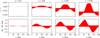Fig. 3 Accuracy of our analytical estimates of e and M0 (see Sect. 4.1) assuming the Fourier decomposition of the signal to be perfectly known. We plot the range of deviations from the true eccentricity (top) and mean anomaly (bottom) as a function of the argument of periastron, ω, and the true eccentricity, e.

4.2 Combining astrometric and radial velocity time series

The method described in Sect. 4.1 to derive an estimate of the eccentricity, e, and of the mean anomaly at reference epoch, M₀, can be extended to the case of a combination of astrometric and radial velocity time series in a straightforward way. We still assume that the orbital period of the companion has been correctly determined with the periodogram approach and we define a linear model including the fundamental frequency (mean motion n = 2π/P) and the first harmonics (2n), for both time series:

$$\begin{array}{lll}{\phi }_{\text{a}}\hfill & =\hfill & ({\phi }_{H,\text{a}},\hfill \\ \hfill & \hfill & \cos \theta \cos n{t}_{\text{a}},sin\theta \cos n{t}_{\text{a}},\hfill \\ \hfill & \hfill & \cos \theta sinn{t}_{\text{a}},sin\theta sinn{t}_{\text{a}},\hfill \\ \hfill & \hfill & \cos \theta \cos 2n{t}_{\text{a}},sin\theta \cos 2n{t}_{\text{a}},\hfill \\ \hfill & \hfill & \cos \theta sin2n{t}_{\text{a}},sin\theta sin2n{t}_{\text{a}}),\hfill \\ {\beta }_{\text{a}}\hfill & =\hfill & ({\beta }_{H,\text{a}},\hfill \\ \hfill & \hfill & {\beta }_{\delta ,1,c},{\beta }_{\alpha ,1,c},\hfill \\ \hfill & \hfill & {\beta }_{\delta ,1,s},{\beta }_{\alpha ,1,s},\hfill \\ \hfill & \hfill & {\beta }_{\delta ,2,c},{\beta }_{\alpha ,2,c},\hfill \\ \hfill & \hfill & {\beta }_{\delta ,2,s},{\beta }_{\alpha ,2,s},),\hfill \\ {\phi }_{\text{rv}}\hfill & =\hfill & ({\phi }_{H,\text{rv}},\hfill \\ \hfill & \hfill & \cos n{t}_{\text{rv}},sinn{t}_{\text{rv}},\hfill \\ \hfill & \hfill & \cos 2n{t}_{\text{rv}},sin2n{t}_{\text{rv}}),\hfill \\ {\beta }_{\text{rv}}\hfill & =\hfill & ({\beta }_{H,\text{rv}},\hfill \\ \hfill & \hfill & {\beta }_{\text{rv,1,}c},{\beta }_{\text{rv,1,}s},\hfill \\ \hfill & \hfill & {\beta }_{\text{rv,2,}c},{\beta }_{\text{rv,2,}s}).\hfill \end{array}$$(52)

We obtain the best-fitting parameters β_a, β_rv, as well as the covariance matrices $C_{{\beta }_{\text{a}}},C_{{\beta }_{\text{rv}}}$ by minimizing the corresponding χ². We derive the values of ρ_δ, ρ_α, η_δ, η_α (see Eqs. (42)-(41)) from the astrometric parameters β_a. We also derive (see Delisle et al. 2016):

$$\begin{array}{lll}{\rho }_{\text{rv}}\hfill & =\hfill & \frac{V_2}{V_1},\hfill \\ {\eta }_{\text{rv}}\hfill & =\hfill & \frac{V_2}{V_1^2},\hfill \end{array}$$(53)

with

$$\begin{array}{lll}{V}_1\hfill & =\hfill & \frac{1}{2}\left({\beta }_{\text{rv,1,}c}-\text{i}{\beta }_{\text{rv,1,}s}\right),\hfill \\ V_2\hfill & =\hfill & \frac{1}{2}\left({\beta }_{\text{rv,2,}c}-\text{i}{\beta }_{\text{rv,2,}s}\right).\hfill \end{array}$$(54)

We then use the method described in Delisle et al. (2016) and Sect. 4.1 to obtain the estimates ê_k and ${\widehat{M}}_{0k}$ from the values of ρ_k and η_k (k = δ, α, rv). These three estimates are finally combined to obtain ê and ${\widehat{M}}_0$, using the error propagation and weighting method detailed in Appendix C.

Following the same line as in Sect. 4.1, we performed a linear fit of the astrometric time series to obtain estimates of the Thiele-Innes coefficients (A, B, F, and G). Similarly, we performed a linear fit of the radial velocity time series to obtain estimates of K_c = K cos ω and K_s = K sin ω. These estimates should again be combined to obtain a set of four parameters describing the orbit, in addition to the three parameters already determined (P, e, M₀).

The astrometry is sensitive to all the orbital parameters but has a degeneracy between two symmetric solutions for the argument of periastron ω and the longitude of the node Ω (ω′ = ω + π, Ω′ = Ω + π). On the contrary, the radial velocities are not sensitive to the inclination, i, and the longitude of the node, Ω, but allow us to break the degeneracy by providing an estimate of the argument of periastron, ω. To combine the parameters obtained from astrometry and radial velocities, we introduce the following parameters:

$$\begin{array}{lll}U\hfill & =\hfill & {\left(a_{s,\text{AU}}\sin i\right)}^2\cos 2\omega ,\hfill \\ V\hfill & =\hfill & {\left(a_{s,\text{AU}}\sin i\right)}^{2}sin2\omega .\hfill \end{array}$$(55)

These parameters can be derived both from the astrometric parameters,

$$\begin{array}{lll}{\widehat{U}}_{\text{a}}\hfill & =\hfill & \frac{\left({\widehat{A}}^2+{\widehat{B}}^2\right)-\left({\widehat{F}}^2+{\widehat{G}}^2\right)}{{\varpi }^2},\hfill \\ {\widehat{V}}_{\text{a}}\hfill & =\hfill & -2\frac{\widehat{A}\widehat{F}+\widehat{B}\widehat{G}}{{\varpi }^2},\hfill \end{array}$$(56)

and the radial velocity parameters,

$$\begin{array}{lll}{\widehat{U}}_{\text{rv}}\hfill & =\hfill & \frac{1-{\widehat{e}}^2}{{\widehat{n}}^2}\left({\widehat{K}}_c^2-{\widehat{K}}_s^2\right),\hfill \\ {\widehat{V}}_{\text{rv}}\hfill & =\hfill & 2\frac{1-{\widehat{e}}^2}{{\widehat{n}}^2}{\widehat{K}}_c{\widehat{K}}_s.\hfill \end{array}$$(57)

We followed the same approach as in Appendix C to propagate the covariance matrices of the linear fits and performed a weighted average of the two estimates of U and V. From the weighted estimates Û, $\widehat{V}$ it is straightforward to derive estimates for a_s sin i and ω. For the argument of periastron, ω, two solutions are actually possible since U and V depend on 2ω, but we chose the one that is closest to the radial velocity estimate (obtained from ${\widehat{K}}_c,{\widehat{K}}_s$). The two remaining parameters only depend on the astrometry and can be chosen arbitrarily. For instance, Ω can be estimated with

$$\widehat{\text{Ω}}=\arctan \left(\widehat{B}\cos \omega -\widehat{G}\sin \omega ,\widehat{A}\cos \omega -\widehat{F}\sin \omega \right),$$(58)

and cos i can be estimated using (e.g., Popovic & Pavlović 1995):

$$\cos \widehat{i}=\frac{m}{k+j},$$(59)

with

$$\begin{array}{l}m=\widehat{A}\widehat{G}-\widehat{B}\widehat{F}\approx a_s^2\cos i,\hfill \\ k=\frac{1}{2}\left({\widehat{A}}^2+{\widehat{B}}^2+{\widehat{F}}^2+{\widehat{G}}^2\right)\approx a_s^2\frac{1+{\cos }^{2}i}{2},\hfill \\ j=\sqrt{k^2-m^2}\approx a_s^2\frac{si{n}^{2}i}{2}.\hfill \end{array}$$(60)

5 Applications

We go on to illustrate our methods with a reanalysis of the astrometric and radial velocity time series of three stars known to host a companion: HD 223636 (HIP 117622), HD 17289 (HIP 12726), and HD 3277 (HIP 2790). We used Hipparcos data (with the reduction of van Leeuwen 2007) for the astrometry and CORALIE data for the radial velocities. We binned Hipparcos data over one-day intervals and excluded the bins with a resulting uncertainty larger than 2.5 mas.

An upgrade of CORALIE was performed in 2007 to improve the overall transmission of the instrument. This upgrade affected the instrumental zero point and the overall instrument stability (Ségransan et al. 2010). We thus actually considered the data taken before and after the upgrade as coming from two different instruments (COR98 before and COR07 after). We modeled the noise as the quadratic sum of the individual measurements errors, as provided by the instruments reduction pipelines, and an additional instrumental jitter: ${\tilde{\sigma }}_i=\sqrt{{\sigma }_i^2+{\sigma }_{\text{inst.}}^2}$. Such a modeling process allows us to account for both stellar and instrumental noises that are not already modeled by the reduction pipelines. We thus defined three jitter terms: σ_HIP for Hipparcos data and then σ_COR98 and σ_COR07 for CORALIE data. We initially set the default values σ_COR98 = 5 m s⁻¹ and σ_COR07 = 8 m s⁻¹, which correspond to the observed scatter of a set of bright and stable solar type stars monitored on a regular basis with CORALIE since 1998. For Hipparcos, we used a default value of σ_HIP = 0 mas. We let the three jitter values vary at the end of the analysis to adapt to the specificity of each dataset.

We applied a similar procedure for each target, using our open source python package kepmodel². We analyzed the astrometric and radial velocity time series both independently and jointly. We computed the periodogram and associated FAP according to Delisle et al. (2020a) (radial velocities) and Sect. 3 (astrometry and joint analysis). All the periodograms were computed using the normalized power of Eq. (22) and by sampling the angular frequency linearly in the range [2π/50 000, 2π/0.9] (rad day⁻¹) with 50 000 values, such that the oversampling factor is always above 10. We then extracted from the periodogram the period corresponding to the highest peak and applied our analytical methods to estimate the other orbital parameters, using Delisle et al. (2016; radial velocities) and Sect. 4 (astrometry and joint analysis). We then adjusted the values of all the parameters by performing a local maximization of the likelihood ℒ using the L-BFGS-B algorithm provided by the scipy python package. This algorithm makes use of the partial derivatives of the likelihood with respect to the parameters, which we computed analytically. We estimated errorbars on the parameters by extracting the diagonal of the inverse of the Hessian matrix of the likelihood. We then repeated the fitting procedure but additionally adjusting the values of the instrumental jitter terms. Finally, we computed the periodograms and FAP of the residuals of the joint model, considering the astrometric and radial velocity time series independently or jointly.

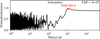Fig. 4 Periodogram of the Hipparcos astrometric time series of HD 223636.

5.1 HD 223636

We first considered HD 223636 (HIP 117622), which was found to host a companion at about 1008 days by Goldin & Makarov (2007), based on an analysis of the Hipparcos time series. No radial velocities are available for this target and we thus only reanalyzed the Hipparcos time series. The periodogram of the astrometric data is shown in Fig. 4, where we clearly see a very significant peak (FAP = 3 × 10⁻⁵) around 1050 days.

We show in Table 2 the parameters obtained using our analytical estimation method (initial guess), after a local maximization of the likelihood and after a second fit, including the jitter term. We observe that the initial guess of the parameters is very close to the maximum likelihood estimate. When adjusting the jitter, we obtain a value of about 0.64 mas, while the average Hipparcos errorbar (over one day bins) is about 0.93 mas. Accounting for this jitter significantly increases the uncertainties on all the parameters, and allows to have a better assessment of the actual precision on these parameters. We note that the final uncertainty on the argument of periastron, ω, is large (29 deg), while the other angles have errorbars below 5 deg. The set of parameters is chosen as to avoid strong correlations between these angles. In particular, the phase of the planet on its orbit is modeled using the mean argument at the reference epoch M₀ + ω instead of the mean anomaly M₀ (which is anti-correlated with ω) or the mean longitude λ₀ = M₀ + ω + Ω (which is correlated with Ω). The astrometric orbit corresponding to the maximum likelihood parameters (including jitter), is shown in Fig. 5 superimposed with Hipparcos measurements. The periodogram of the residuals is shown in Fig. 6, where no significant peak is found (FAP = 0:89).

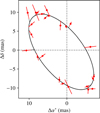Fig. 5 Astrometric orbit of HD 223636.

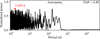Fig. 6 Periodogram of Hipparcos astrometric residuals of HD 223636 after fitting for its companion.

5.2 HD 17289

The second target, HD 17289 (HIP 12726), was also found to host a companion by Goldin & Makarov (2007) using Hipparcos astrometry alone. The companion was later confirmed and better characterized by Sahlmann et al. (2011) using both Hipparcos astrometry and CORALIE radial velocities. This system is actually a binary star, with a mass ratio of about 2 between the primary and the companion, leading to a contrast of about 1 : 180 in the visible, which slightly affects the radial-velocity measurements. This issue is discussed in details in Sahlmann et al. (2011) and is beyond the scope of our study. Here, we use the same Hipparcos and CORALIE data as Sahlmann et al. (2011). The CORALIE data consist of 29 measurements (22 COR98 and 7 COR07).

We show in Fig. 7 the periodogram of the astrometric data alone, the radial velocities alone, as well as the joint periodogram. In the three cases, a significant peak is detected around 570 days. Since the time span of CORALIE measurements (11.3 yr) is much longer than the time span of Hipparcos measurements (3.2 yr), the radial velocity peak is much narrower. The joint periodogram shows a very similar shape as the radial velocity periodogram, but provides stronger evidence for the existence of a companion (FAP = 3 × 10⁻⁸ and 10⁻³, respectively).

Table 3 provides the parameters obtained at the different steps of our procedure using astrometry alone, radial velocities alone, and both datasets together. In all three cases, our analytical method provides a good initial guess of the parameters. When using the radial velocities alone, the provided value for the semi-major axis, a_s, is actually the minimum semi-major axis (a_s sin i), which is equivalent to assuming an inclination of 90 deg. Since the actual inclination is about 174 deg (sin i ≈ 0.1), this explains the factor of 10 difference with regard to the astro-metric or joint value. The other parameters show coherent values between astrometry and radial velocities. When using astrometric data alone, the parameters ω and Ω present two degenerated solutions (ω, Ω) and (ω + π, Ω + π). In order to ease the comparisons, we chose the solution that is the closest to the value of ω obtained with radial velocities. However, it should be kept in mind that there is no way to break this degeneracy using astrometry alone. We observe that while the inclination, i, and longitude of the node Ω are not constrained by radial velocities, we obtain a much higher precision on these parameters with the joint fit than using astrometry alone. This is because of the correlations between these two parameters and the other orbital parameters, which are much better constrained by the radial velocities than the astrometry.

The astrometric orbit corresponding to the maximum likelihood parameters (including jitter), superimposed with Hipparcos measurements, is shown in Fig. 8, while the phase-folded radial velocity model, superimposed with CORALIE measurements, is shown in Fig. 9. Finally, the periodograms of the residuals are shown in Fig. 10, where no significant peak is found (FAP > 0.66).

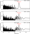Fig. 7 Periodograms of the Hipparcos time series (astrometry, top), CORALIE time series (RV, middle), and joint periodogram (bottom) of HD 17289.

5.3 HD 3277

The last system we analyzed is HD 3277 (HIP 2790). It was first listed by Tokovinin et al. (2006) as an uncertain spectroscopic binary based on few CORALIE measurements and Sahlmann et al. (2011) confirmed the presence of a companion using additional CORALIE measurements as well as Hipparcos data. The primary component is a G8 star while the companion is an M-dwarf. We analyzed the same data as in Sahlmann et al. (2011), namely, Hipparcos data and 14 CORALIE measurements (10 COR98 and 4 COR07).

The periodograms and FAP of the astrometric and radial velocity time series are shown in Fig. 11. We observe a nonsignificant peak around 46 days in the radial velocities periodogram (FAP = 0.16). This high FAP value can be explained by the poor sampling of the radial velocity time series, which consists of only 14 points split among two instruments. To test this hypothesis, we recomputed the periodogram and FAP of the radial velocity time series but assuming the offset between COR98 and COR07 to be negligible, and found a more significant FAP of 0.015. A peak is also visible in the astrometric periodogram at the same period, but it is not the highest one, and the FAP is very high (0.73). The joint periodogram is very similar in shape to the radial velocities periodogram but the associated FAP is significantly lower (5 × 10⁻⁸).

Since the 46 days signal is not detected using astrometry alone, we only applied our procedure to the radial velocities and the joint model. The parameters we obtained are shown in Table 4. As for previous systems, our analytical method provides a good initial guess of the parameters, which is then refined by maximizing the likelihood. The most challenging parameter is the inclination, which is only constrained by the astrometry, for which the initial guess is within 40 deg of the maximum likelihood value. This slight discrepancy is not surprising considering the low S/N of the signal in the astrometric time series (high FAP, other more significant peaks in the periodogram). The maximum likelihood astrometric and radial velocity models, superimposed with the corresponding data, are shown in Figs. 12 and 13. The periodograms of the residuals are shown in Fig. 14, where no significant peak is found (FAP > 0.77).

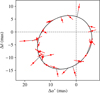Fig. 8 Astrometric orbit of HD 17289.

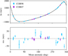Fig. 9 Phase-folded RV time series of HD 17289.

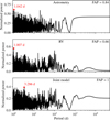Fig. 10 Periodograms of the residuals of the Hipparcos time series (astrometry, top), CORALIE time series (RV, middle), and joint peri-odogram (bottom) of HD 17289, after fitting for its companion.

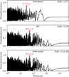Fig. 11 Periodograms of the Hipparcos time series (astrometry, top), CORALIE time series (RV, middle), and joint periodogram (bottom) of HD 3277, after fitting for its companion.

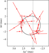Fig. 12 Astrometric orbit of HD 3277.

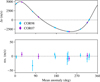Fig. 13 Phase-folded RV time series of HD 3277.

6 Discussion

In this work, we present a set of methods to detect and characterize companions (planets, brown dwarfs, and stars) in astrometric or radial velocity time series, or both. We propose a general linear periodogram framework with an analytical method to compute the associated FAP. We additionally provide an analytical method to obtain an estimate of the orbital parameters once the period of the companion has been determined (from the periodogram approach). These methods can be applied to astrometric data alone, radial velocities alone, but also when combining both detection techniques.

Being based on analytical approximations, our methods are very efficient in terms of computational cost. This is of particular interest in the context of the Gaia space mission, considering the amount of generated data. It should be noted that these approximate analytical methods are complementary with more precise numerical methods. For instance, in Sect. 5, we use our analytical estimate of the orbital parameters as a starting point for a likelihood maximization algorithm. More generally, both the periodogram-FAP approach and the orbital parameters approximation can be used to improve the convergence speed of numerical algorithms, such as Markov chain Monte-Carlo, genetic algorithms, and so on. In particular, our analytical estimate of orbital parameters has been implemented in the genetic algorithm of the official Gaia pipeline for the detection of planets (MIKS-GA, see Holl et al. 2022).

Indeed, a primary objective of this article is to provide building blocks for the detection and characterization of planets using Gaia astrometry alone as well as in combination with on-ground radial velocities. Since the Gaia collaboration will not publish astrometric time series before DR4, we were not able to illustrate our methods on Gaia sources hosting planetary companions. We instead chose to reanalyze the Hipparcos astrometric time series of three stars known to host a stellar companion: HD 223636 (HIP 117622), HD 17289 (HIP 12726), and HD 3277 (HIP 2790). Using Hipparcos astrometry and publicly available CORALIE radial velocities, we obtained results similar to the literature. In these examples, we found that the joint periodograms (astrometry + radial velocities) were very similar to the periodogram of the radial velocity alone. This is because the S/N of the companion is much higher in CORALIE radial velocities than in Hipparcos astrometry. Therefore, a combined periodogram might not actually appear necessary to find the companion period in these cases. However, since Gaia will provide much higher precision astrometric time series and with a much longer time span than Hipparcos, the contribution of astrometry and radial velocities will be more balanced.

Finally, it should be noted that while we assume white noise in our illustrations (Sect. 5), our methods are derived in the more general case of correlated noise. Indeed, radial velocities are known to be affected by stellar activity, which is often modeled using Gaussian processes (i.e., correlated noise models). Other sources of noise, such as the spectrograph calibration noise, can also introduce correlated noise in the radial velocity time series (e.g., Delisle et al. 2020b). In the case of astrometric data, the stellar activity signature is expected to be much smaller than for radial velocities (Lagrange et al. 2011). However, the attitude calibration of the satellite might introduce correlated noise in the astrometric time series. In the case of Gaia, the correlated noise contribution remains to be investigated and characterized, but once this is done, our framework is readily equipped to account for it.

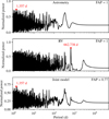Fig. 14 Periodograms of the residuals of the Hipparcos time series (astrometry, top), CORALIE time series (RV, middle), and joint periodogram (bottom) of HD 3277, after fitting for its companion.

Acknowledgements

We thank the anonymous referee for their very constructive feedback that helped to improve this manuscript. We acknowledge financial support from the Swiss National Science Foundation (SNSF). This work has, in part, been carried out within the framework of the National Centre for Competence in Research PlanetS supported by SNSF.

Appendix A Power fraction in the fundamental and harmonics

In this appendix, we compute the power fraction that is found in the fundamental and in the harmonics for a radial velocity (Appendix A.1) and an astrometric Keplerian signal (Appendix A.2).

A.1 Radial velocity signal

We follow Baluev (2015) to define the total power of a Keplerian radial velocity signal V_K(t) = K(cos(v(t) + ω) + e cos ω) as:

$$\begin{array}{lll}{P}_{\text{tot.}}\hfill & =\hfill & \frac{1}{P}{\displaystyle {\int }_0^P{V}_K^2\left(t\right)dt}\hfill \\ \hfill & =\hfill & \frac{K^2}{2}\left(1-e^2\right)\left(1-{\beta }^2\cos 2\omega \right),\hfill \end{array}$$(A.1)

where

$$\beta =\frac{e}{1+\sqrt{1-e^2}},$$(A.2)

and v is the true anomaly. The Fourier expansion of this signal is (e.g., Delisle et al. 2016):

$$\begin{array}{lll}{V}_0\hfill & =\hfill & 0,\hfill \\ V_k\hfill & =\hfill & \frac{K{\text{e}}^{\text{i}k{M}_0}}{2}\left(X_k{\text{e}}^{\text{i}\omega }+X_{-k}{\text{e}}^{-\text{i}\omega }\right)\left(k\ne 0\right),\hfill \end{array}$$(A.3)

where X_k is the Hansen coefficient $X_k^{0,1}$ which only depends on the eccentricity e and is defined has

$$X_k\left(e\right)=\frac{1}{2\pi }{\displaystyle {\int }_0^{2\pi }{\text{e}}^{\text{i}v}{\text{e}}^{-\text{i}kM}\text{d}M.}$$(A.4)

The power in the harmonics are thus:

$$P_0=0,$$(A.5)

$$\begin{array}{cc}{P}_k=2V_k{\overline{V}}_k=\frac{K^2}{2}\left(X_k^2+X_{-k}^2+2X_k{X}_{-k}\cos 2\omega \right)& \left(k>0\right).\end{array}$$

Finally the power fraction in the k-th harmonics (k > 0) is:

$$R_k=\frac{P_k}{P_{\text{tot.}}}=\frac{X_k^2+X_{-k}^2+2X_k{X}_{-k}\cos 2\omega }{\left(1-e^2\right)\left(1-{\beta }^2\cos 2\omega \right)}.$$(A.6)

As shown by Baluev (2015), the ratio R₁ is linked with the detection efficiency of the classical periodogram (which only uses the fundamental frequency) compared to a more complex Keplerian periodogram (which uses the full information contained in the signal).

The power fraction R_k depends on the eccentricity and (weakly) on the argument of periastron. For a given eccentricity, the extrema of the power fraction correspond to 2ω = 0 or π. We define

$$\begin{array}{lll}{R}_k^{+}\hfill & =\hfill & \frac{X_k^2+X_{-k}^2+2X_k{X}_{-k}}{\left(1-e^2\right)\left(1-{\beta }^2\right)},\hfill \\ R_k^{-}\hfill & =\hfill & \frac{X_k^2+X_{-k}^2-2X_k{X}_{-k}}{\left(1-e^2\right)\left(1+{\beta }^2\right)},\hfill \end{array}$$(A.7)

such that R_k is always between $R_k^{+}$ and $R_k^{-}$ (the order depending on k and e). In Fig. 2, we plot the possible range of values of R_k as a function of the eccentricity, for k = 1,2 (fundamental and first harmonics). For this plot, we evaluated the Hansen coefficients by numerical integration over the eccentric anomaly (see Delisle et al. 2016, Appendix A).

A.2 Astrometric signal

Here, we follow the same approach as in the radial velocity case. Since the astrometric signal has two dimensions, we define the total power of the signal as the sum of powers along both directions:

$$\begin{array}{lll}{P}_{\text{tot.}}\hfill & =\hfill & \frac{1}{P}{\displaystyle {\int }_0^P\left({\delta }_K^2\left(t\right)+{\alpha }_K^2\left(t\right)\right)\text{d}t}\hfill \\ \hfill & =\hfill & \frac{1}{2\pi }{\displaystyle {\int }_0^{2\pi }\left({\left(Ax+Fy\right)}^2+{\left(Bx+Gy\right)}^2\right)\text{d}M}.\hfill \end{array}$$(A.8)

We have

$$\begin{array}{lll}\frac{1}{2\pi }{\displaystyle {\int }_0^{2\pi }{x}^2\text{d}M}\hfill & =\hfill & \frac{1}{2\pi }{\displaystyle {\int }_0^{2\pi }{x}^2\left(1-e\cos E\right)\text{d}E}\hfill \\ \hfill & =\hfill & \frac{1}{2\pi }{\displaystyle {\int }_0^{2\pi }{\left(\cos E-e\right)}^2\left(1-e\cos E\right)}\text{\hspace{0.17em}d}E\hfill \\ \hfill & =\hfill & \frac{1}{2}+2e^2,\hfill \end{array}$$(A.9)

$$\begin{array}{lll}\frac{1}{2\pi }{\displaystyle {\int }_0^{2\pi }{y}^2\text{d}M}\hfill & =\hfill & \frac{1-e^2}{2\pi }{\displaystyle {\int }_0^{2\pi }{\sin }^{2}E\left(1-e\cos E\right)\text{d}E}\hfill \\ \hfill & =\hfill & \frac{1-e^2}{2},\hfill \end{array}$$(A.10)

$$\begin{array}{lll}\frac{1}{2\pi }{\displaystyle {\int }_0^{2\pi }xy\text{d}M}\hfill & =\hfill & \frac{\sqrt{1-e^2}}{2\pi }{\displaystyle {\int }_0^{2\pi }\left(\cos E-e\right)\sin E\left(1-e\cos E\right)\text{d}E}\hfill \\ \hfill & =\hfill & 0,\hfill \end{array}$$(A.11)

thus:

$$\begin{array}{lll}{P}_{\text{tot.}}\hfill & =\hfill & \left(\frac{1}{2}+2e^2\right)\left(A^2+B^2\right)+\frac{1-e^2}{2}\left(F^2+G^2\right)\hfill \\ \hfill & =\hfill & \frac{a_s^2}{4}\left(\left(2+3e^2\right)\left(2-{\sin }^{2}i\right)+5e^2{\sin }^{2}i\cos 2\omega \right).\hfill \end{array}$$(A.12)

The Fourier expansion of δ_K and α_K is provided in Eqs. (8), (14), from which we deduce the power in the k-th harmonics (k > 0):

$$\begin{array}{lll}{P}_k\hfill & =\hfill & 2{\delta }_k{\overline{\delta }}_k+2{\alpha }_k{\overline{\alpha }}_k\hfill \\ \hfill & =\hfill & \frac{A^2+B^2+C^2}{2}\left({\zeta }_k^2+{\zeta }_{-k}^2\right)+\left(A^2+B^2-F^2-G^2\right){\zeta }_k{\zeta }_{-k}\hfill \\ \hfill & =\hfill & \frac{a_s^2}{2}\left(\left({\xi }_k^2+{\zeta }_{-k}^2\right)\left(2-{\sin }^{2}i\right)+2{\zeta }_k{\zeta }_{-k}{\sin }^{2}i\cos 2\omega \right).\hfill \end{array}$$(A.13)

In contrast to the case of radial velocities, the Keplerian astro-metric signal is not centered, which implies that the power ofthe constant part (k = 0) is not zero, that is,

$$\begin{array}{lll}{P}_0\hfill & =\hfill & {\delta }_0^2+{\alpha }_0^2={\zeta }_0^2\left(A^2+B^2\right)\hfill \\ \hfill & =\hfill & \frac{9}{8}{a}_s^2{e}^2\left(2-{\sin }^{2}i+{\sin }^{2}i\cos 2\omega \right).\hfill \end{array}$$(A.14)

In practice, the constant part does not contain any information about the companion because the reference position of the primary always needs to be adjusted at the same time as the orbit. Therefore, in the following, we normalize the power in the harmonics by the useful total power:

$$P_{\text{tot.}}-P_0=\frac{a_s^2}{8}\left(\left(4-3e^2\right)\left(2-{\sin }^{2}i\right)+e^2{\sin }^{2}i\cos 2\omega \right),$$(A.15)

which is equivalent to re-centering the Keplerian astrometric model. We then define the power fraction as

$$\begin{array}{lll}{R}_k\hfill & =\hfill & \frac{P_k}{P_{\text{tot.}}-P_0}\hfill \\ \hfill & =\hfill & 4\frac{\left({\zeta }_k^2+{\zeta }_{-k}^2\right)\left(2-{\sin }^{2}i\right)+2{\zeta }_k{\zeta }_{-k}{\sin }^{2}i\cos 2\omega }{\left(4-3e^2\right)\left(2-{\sin }^{2}i\right)+e^2{\sin }^{2}i\cos 2\omega }.\hfill \end{array}$$(A.16)

This fraction depends on e, ω and i. For a given eccentricity, the extrema of the fraction appears for 2ω = 0, π and i = π/2. We thus define

$$\begin{array}{lll}{R}_k^{+}\hfill & =\hfill & 2\frac{{\left({\zeta }_k+{\zeta }_{-k}\right)}^2}{2-e^2},\hfill \\ R_k^{-}\hfill & =\hfill & 2\frac{{\left({\zeta }_k-{\zeta }_{-k}\right)}^2}{1-e^2},\hfill \end{array}$$(A.17)

such that R_k is always between $R_k^{+}$ and $R_k^{-}$. We then need to evaluate the coefficients ζ_k to compute these fractions. We use the same method as for the Hansen coefficient (Appendix A.1). We estimate the integral of Eq. (15) numerically by sampling E in [0, 2π],

$$\begin{array}{lll}{\zeta }_k\hfill & \approx \hfill & \frac{1}{N}{\displaystyle \sum _{j=0}^{N-1}\left(\cos {\dot{E}}_j-e+\text{i}\sqrt{1-e^2}\sin E_j\right)}\hfill \\ \hfill & \hfill & \times {\text{e}}^{-\text{i}k\left(E_j-e\sin E_j\right)}\left(1-e\cos E_j\right),\hfill \end{array}$$(A.18)

References

- Arsenault, R., Alonso, J., Bonnet, H., et al. 2003, SPIE Conf. Ser., 4839, 174 [NASA ADS] [Google Scholar]
- Barrell, K., & Pask, C. 1979, Optica Acta, 26, 91 [NASA ADS] [CrossRef] [Google Scholar]
- Beuzit, J.-L., Vigan, A., Mouillet, D., et al. 2019, A&A, 631, A155 [NASA ADS] [CrossRef] [EDP Sciences] [Google Scholar]
- Brogi, M., & Line, M. R. 2019, AJ, 157, 114 [Google Scholar]
- Brogi, M., Snellen, I., De Kok, R., et al. 2013, ApJ, 767, 27 [NASA ADS] [CrossRef] [Google Scholar]
- Coudé du Foresto, V., Maze, G., & Ridgway, S. 1993, in Astronomical Society of the Pacific Conference Series, Fiber Optics in Astronomy II, ed. P.M. Gray, 37, 285 [Google Scholar]
- Coudé du Foresto, V. 1994, in Very High Angular Resolution Imaging, eds. J.G. Robertson, & W.J. Tango, 158, 261 [CrossRef] [Google Scholar]
- Crepp, J. R. 2014, Science, 346, 809 [NASA ADS] [CrossRef] [Google Scholar]
- Crepp, J. R., Johnson, J. A., Fischer, D. A., et al. 2012, ApJ, 751, 97 [Google Scholar]
- de Kok, R. J., Brogi, M., Snellen, I. A., et al. 2013, A&A, 554, A82 [NASA ADS] [CrossRef] [EDP Sciences] [Google Scholar]
- Delorme, J.-R., Jovanovic, N., Echeverri, D., et al. 2021, J. Astron. Telescopes Instrum. Syst., 7, 035006 [NASA ADS] [Google Scholar]
- Dorn, R. J., Follert, R., Bristow, P., et al. 2016, in Ground-based and Airborne Instrumentation for Astronomy VI, International Society for Optics and Photonics, 9908, 99080I [Google Scholar]
- Fusco, T., Rousset, G., Sauvage, J.-F., et al. 2006, Opt. Express, 14, 7515 [NASA ADS] [CrossRef] [Google Scholar]
- Ghasempour, A., Kelly, J., Muterspaugh, M. W., & Williamson, M. H. 2012, in Modern Technologies in Space-and Ground-based Telescopes and Instrumentation II, International Society for Optics and Photonics, 8450, 845045 [NASA ADS] [Google Scholar]
- Gibson, R. K., Oppenheimer, R., Matthews, C. T., & Vasisht, G. 2020, J. Astron. Telescopes Instrum. Syst., 6, 011002 [NASA ADS] [Google Scholar]
- Guyon, O., Pluzhnik, E., Kuchner, M. J., Collins, B., & Ridgway, S. 2006, ApJS, 167, 81 [NASA ADS] [CrossRef] [Google Scholar]
- Jeunhomme, L. B. 1983, Single-mode Fiber Optics. Principles and Applications [Google Scholar]
- Jovanovic, N., Martinache, F., Guyon, O., et al. 2015, PASP, 127, 890 [NASA ADS] [CrossRef] [Google Scholar]
- Jovanovic, N., Cvetojevic, N., Schwab, C., et al. 2016, SPIE Conf. Ser., 9908, 99080R [NASA ADS] [Google Scholar]
- Jovanovic, N., Schwab, C., Guyon, O., et al. 2017, A&A, 604, A122 [NASA ADS] [CrossRef] [EDP Sciences] [Google Scholar]
- Kaeufl, H.-U., Ballester, P., Biereichel, P., et al. 2004, SPIE Conf. Ser., 5492, 1218 [NASA ADS] [Google Scholar]
- Kasper, M., Cerpa Urra, N., Pathak, P., et al. 2021, The Messenger, 182, 38 [Google Scholar]
- Kotani, T., Kawahara, H., Ishizuka, M., et al. 2020, in Adaptive Optics Systems VII, International Society for Optics and Photonics, 11448, 1144878 [Google Scholar]
- Lovis, C., Snellen, I., Mouillet, D., et al. 2017, A&A, 599, A16 [NASA ADS] [CrossRef] [EDP Sciences] [Google Scholar]
- Lyot, B. 1933, J. R. Astron. Soc. Canada, 27, 265 [NASA ADS] [Google Scholar]
- Macintosh, B., Graham, J. R., Ingraham, P., et al. 2014, Proc. Natl. Acad. Sci. U.S.A., 111, 12661 [Google Scholar]
- Mawet, D., Pueyo, L., Lawson, P., et al. 2012, in Space Telescopes and Instrumentation 2012: Optical, Infrared, and Millimeter Wave, eds. M.C. Clampin, G.G. Fazio, H.A. MacEwenJr., & J.M.O., International Society for Optics and Photonics (SPIE), 8442, 62 [Google Scholar]
- Mawet, D., Ruane, G., Xuan, W., et al. 2017, ApJ, 838, 92 [Google Scholar]
- Mayor, M., & Queloz, D. 1995, Nature, 378, 355 [Google Scholar]
- McLean, I. S., Becklin, E. E., Bendiksen, O., et al. 1998, in Infrared Astronomical Instrumentation, International Society for Optics and Photonics, 3354, 566 [NASA ADS] [CrossRef] [Google Scholar]
- N’Diaye, M., Dohlen, K., Cuevas, S., et al. 2010, A&A, 509, A8 [NASA ADS] [CrossRef] [EDP Sciences] [Google Scholar]
- N’Diaye, M., Dohlen, K., Cuevas, S., et al. 2012, A&A, 538, A55 [NASA ADS] [CrossRef] [EDP Sciences] [Google Scholar]
- N’Diaye, M., Dohlen, K., Fusco, T., & Paul, B. 2013, A&A, 555, A94 [NASA ADS] [CrossRef] [EDP Sciences] [Google Scholar]
- Neumann, E.-G. 1988, in Single-Mode Fibers (Springer), 210 [CrossRef] [Google Scholar]
- Otten, G., Vigan, A., Muslimov, E., et al. 2021, A&A, 646, A150 [NASA ADS] [CrossRef] [EDP Sciences] [Google Scholar]
- Paul, B., Mugnier, L., Sauvage, J.-F., Dohlen, K., & Ferrari, M. 2013, Opt. Express, 21, 31751 [NASA ADS] [CrossRef] [Google Scholar]
- Piso, A.-M.A., Pegues, J., & Öberg, K.I. 2016, ApJ, 833, 203 [NASA ADS] [CrossRef] [Google Scholar]
- Pourcelot, R., Vigan, A., Dohlen, K., et al. 2021, A&A, 649, A170 [NASA ADS] [CrossRef] [EDP Sciences] [Google Scholar]
- Riaud, P., & Schneider, J. 2007, A&A, 469, 355 [NASA ADS] [CrossRef] [EDP Sciences] [Google Scholar]
- Service, M., Lu, J. R., Campbell, R., et al. 2016, PASP, 128, 095004 [NASA ADS] [CrossRef] [Google Scholar]
- Shaklan, S., & Roddier, F. 1988, Appl. Opt., 27, 2334 [NASA ADS] [CrossRef] [Google Scholar]
- Snellen, I. A., De Kok, R. J., De Mooij, E. J., & Albrecht, S. 2010, Nature, 465, 1049 [NASA ADS] [CrossRef] [Google Scholar]
- Snellen, I. A., Brandl, B. R., De Kok, R. J., et al. 2014, Nature, 509, 63 [NASA ADS] [CrossRef] [Google Scholar]
- Snellen, I., de Kok, R., Birkby, J. L., et al. 2015, A&A, 576, A59 [NASA ADS] [CrossRef] [EDP Sciences] [Google Scholar]
- Soummer, R., Aimé, C., & Falloon, P. 2003a, A&A, 397, 1161 [CrossRef] [EDP Sciences] [Google Scholar]
- Soummer, R., Dohlen, K., & Aime, C. 2003b, A&A, 403, 369 [NASA ADS] [CrossRef] [EDP Sciences] [Google Scholar]
- Soummer, R., Ferrari, A., Aime, C., & Jolissaint, L. 2007, ApJ, 669, 642 [Google Scholar]
- Vigan, A., Bonnefoy, M., Ginski, C., et al. 2016, A&A, 587, A55 [NASA ADS] [CrossRef] [EDP Sciences] [Google Scholar]
- Vigan, A., Otten, G., Muslimov, E., et al. 2018, in Ground-based and Airborne Instrumentation for Astronomy VII, International Society for Optics and Photonics, 10702, 1070236 [Google Scholar]
- Virtanen, P., Gommers, R., Oliphant, T. E., et al. 2020, Nat. Methods, 17, 261 [Google Scholar]
- Wang, J., Mawet, D., Ruane, G., Hu, R., & Benneke, B. 2017, AJ, 153, 183 [Google Scholar]
- Wildi, F. P., Michaud, B., Crausaz, M., et al. 2010, SPIE Conf. Ser., 7735, 77352V [NASA ADS] [Google Scholar]
- Yelda, S., Lu, J. R., Ghez, A. M., et al. 2010, ApJ, 725, 331 [NASA ADS] [CrossRef] [Google Scholar]
- Zurlo, A., Vigan, A., Mesa, D., et al. 2014, A&A, 572, A85 [NASA ADS] [CrossRef] [EDP Sciences] [Google Scholar]
- Zurlo, A., Vigan, A., Galicher, R., et al. 2016, A&A, 587, A57 [NASA ADS] [CrossRef] [EDP Sciences] [Google Scholar]
MIKS-GA: multiple independent Keplerian solution using a Genetic algorithm.
All Tables
False alarm probability for the GLS periodogram (see Eq. (22)) following the method of Baluev (2008).
False alarm probability for the two definitions (Eqs. (22), (B.1)) of the periodogram power (see Baluev 2008).