| Issue |
A&A
Volume 675, July 2023
|
|
|---|---|---|
| Article Number | A124 | |
| Number of page(s) | 7 | |
| Section | Numerical methods and codes | |
| DOI | https://doi.org/10.1051/0004-6361/202245803 | |
| Published online | 11 July 2023 | |
Model-independent periodogram for scanning astrometry
1
Porter School of the Environment and Earth Sciences, Raymond and Beverly Sackler Faculty of Exact Sciences, Tel Aviv University,
Tel Aviv
6997801, Israel
e-mail: This email address is being protected from spambots. You need JavaScript enabled to view it.
2
Department of Particle Physics and Astrophysics, Weizmann Institute of Science,
Rehovot
7610001, Israel
Received:
27
December
2022
Accepted:
6
June
2023
Abstract
We present a new periodogram for the periodicity detection in one-dimensional time-series data from scanning astrometry space missions such as HIPPARCOS or Gaia. The periodogram is non-parametric and does not rely on a full or approximate orbital solution. Since no specific properties of the periodic signal are assumed, the method is expected to be suitable for the detection of various types of periodic phenomena, from highly eccentric orbits to periodic variability-induced movers. The periodogram is an extension of the phase-distance correlation periodogram we introduced in previous papers based on the statistical concept of distance correlation. We demonstrate the performance of the periodogram using publicly available HIPPARCOS data, as well as simulated data. We also discuss its applicability for Gaia epoch astrometry that is to be published in the future data release 4.
Key words: methods: data analysis / methods: statistical / astrometry / binaries: general / planets and satellites: detection
© The Authors 2023
 Open Access article, published by EDP Sciences, under the terms of the Creative Commons Attribution License (https://creativecommons.org/licenses/by/4.0), which permits unrestricted use, distribution, and reproduction in any medium, provided the original work is properly cited.
This article is published in open access under the Subscribe to Open model. This email address is being protected from spambots. You need JavaScript enabled to view it. to support open access publication.
1 Introduction
Major astrometric survey space missions such as HIPPARCOS and Gaia provide position and parallax measurements for a large number of celestial objects (Perryman et al. 1997; Gaia Collaboration 2016). Both missions monitor the sky following a complex scanning law, yielding a sparse unevenly sampled astrometric time series of the various targets (van Leeuwen & Evans 1998; Gaia Collaboration 2016). This scanning is performed along reference great circles (RGC), gradually covering the entire celestial sphere. Thus, in each epoch, an object location is conveyed by two quantities: the scanning angle θ, and the abscissa v.
In its original meaning, the Latin word 'abscissa' refers to the horizontal coordinate in a two-dimensional Cartesian system. In the context of scanning astrometry, the word abscissa refers to one-dimensional positional coordinates that are measured along the scanning direction of the instrument. While scanning astrometry provides well-constrained abscissae, positional measurements in the cross-scan direction, perpendicular to the scanning direction, are obtained with significantly lower precision. As a result, scanning astrometry data are often considered one-dimensional positional measurements. The information they convey is only partial information regarding the astrometric position, while the actual position lies somewhere on an imaginary line perpendicular to the scanning direction. We note that the abscissa is often specified with respect to the catalogue nominal position. Figure 1 illustrates the geometric setting described above.
Full astrometric solutions for the observed targets include several parameters fitted to minimize the model errors in terms of the abscissa residuals (see Perryman et al. 1997; ESA 1997). In the simplest cases, the basic 5-parameter solution (right ascension, declination, two-dimensional proper motion vector, and parallax) is sufficient to model the target's proper motion combined with the apparent motion induced by the motion of Earth. When considering the astrometric motion of a binary system, 7 or 9 parameters are required to account for the target's acceleration. In some cases, if the orbital period is sufficiently short, a 12-parameter model is fitted, to fully account for the Keplerian motion of the system. Solving for these parameters is more complicated and might even be quite computationally demanding and prone to errors of various kinds (e.g. van Leeuwen 2007).
With the very high angular precision of modern instruments such as Gaia, the situation might become even more complicated when the binary system includes compact objects, and relativity comes into effect through light deflection and delays (e.g. Halbwachs 2009). Apparent periodic astrometric motion can also occur in unresolved visual double stars, in which one of the components is a periodically pulsating star. In these cases, commonly known as variability-induced movers (VIMs), the photocenter of the two blended stars undergoes a periodic displacement, that is related to the photometric periodic variability (Wielen 1996).
In other types of astronomical observations, such as radial velocities (RVs) or photometry, the measured quantity is simply a scalar. The common procedure in this context is to first look for periodicity. If a periodicity is indeed found and a crude estimate of the period is obtained, then a full characterization of the variability is attempted, such as a Keplerian RV model, an eclipsing-binary model, or a Cepheid light-curve model. The most common approach to the first step, detecting the periodicity, is using a periodogram. A periodogram scans a grid of trial periods (or frequencies) and assigns each one a score. This score quantifies the plausibility that a periodicity exists in the data, assuming this particular trial period.
The most commonly used periodogram for scalar data is probably the generalized Lomb–Scargle (GLS) periodogram, which fits a sinusoidal function to the data and quantifies the goodness of fit (Zechmeister & Kürster 2009). The underlying assumption is that any periodic function can be described as a sum of harmonics, and assuming the first harmonic is the dominant one, the function can be approximated by a sinusoid. However, the case of abscissa data resulting from scanning astrometry is more complicated and requires special treatment. This is mainly related to the fact that every abscissa is measured along a different scanning direction. Therefore, the data cannot be treated in the same way as simple scalar data.
In this work, we present a non-parametric method for detecting periodicity in time series of one-dimensional astrometric data. This periodogram does not search for a specific type of periodic astrometric motion, and it is based on the concept of the phase distance correlation (PDC). Zucker (2018) introduced the PDC periodogram as a new method for detecting periodicity in time-series data. Essentially, for each trial period, the PDC quantifies the statistical dependence between the measured quantity and the phase (according to the trial period), using the recently introduced distance correlation (Székely et al. 2007).
The distance correlation is a measure of the statistical dependence of random variables (as opposed to the correlation coefficient, which is a measure of linear dependence). One of its merits is that the two random variables need not be of the same dimensions and can even be drawn from general metric spaces, not necessarily Euclidean (Lyons 2013). Lyons (2013) showed that if the two metrics involved are of 'strong negative type'(see Zinger et al. 1992), the distance correlation is guaranteed to be applicable as a measure of statistical dependence.
The PDC periodogram as introduced by Zucker (2018), calculates the distance correlation between the analyzed quantity (e.g., the RV) and the phase according to the trial period for each trial period. As Euclidean spaces are themselves of strong negative type (Lyons 2013), Zucker (2019) further formulated and demonstrated the application of the PDC periodogram to two-dimensional astrometry, using the regular Euclidean metric to quantify distances between different measurements.
In the next section, we discuss the specific adaptation of the PDC concept to scanning astrometry. Section 3 demonstrates the application of the new periodogram to HIPPARCOS data, as well as additional simulated data. We conclude in Sect. 4 and discuss the method and its potential for future studies, particularly in the context of Gaia data.
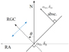 |
Fig. 1 Definition of the abscissa residual v for a single-epoch position (am, δm), with respect to the nominal catalogue position (α0, δ0) and the RGC orientation θ. The actual position of the observed target lies somewhere along the dotted arrowed blue segment. The figure is based on one originally published by van Leeuwen & Evans (1998). |
2 PDC for one-dimensional scanning astrometry
2.1 A new metric
In order to extend the PDC concept to data from scanning astrometry, we had to define a suitable metric for the set of observations using the above-mentioned parameters, the scanning angle θ and abscissa v. This metric should then enable us to estimate the distance correlation measure used to compute the PDC periodogram. After experimenting with a few alternative metrics, we chose the following, which is based on the concept of energy distance.
Energy distance is a statistical distance between probability distributions, first introduced by Gábor Székely (Székely & Rizzo 2013). Note that energy distance is a metric of strong negative type (Rizzo & Székely 2016), and therefore satisfies the sufficient condition for the applicability of distance correlation as an independence test, as mentioned in the previous section.
As shown in Sect. 1, the actual astrometric position of the target can be assumed to lie on a line segment whose length is constrained by the width of the scanning sensor (Fig. 1). We do not have a reason to assume that there is a preference for one particular area of the detector over another, and therefore all points on the segment are a priori equally probable.
In a Bayesian inference setting, we could set a uniform prior for the position along the width of the detector. However, our approach is based on distance correlation and therefore relies on our ability to define a metric between pairs of measurements. To qualitatively reflect the logic of an uninformative prior, we choose to represent each segment only by the position of its edges. This choice defines a one-to-one correspondence between the set of all segments and the set of all unordered pairs of points on the plane.
For the set of all pairs of points on the plane, we can use the energy distance metric in the following way: let U and W be two segments in the plane, which can be represented by their endpoints: u1, u2 and w1,w2, respectively. We can then consider each segment as a sample of two points and calculate the energy distance between the two samples corresponding to U and W (Székely & Rizzo 2013):
 (1)
(1)
We note that |u1 – u2| is the length of the segment U. Now, let the two segments be defined by the abscissae v1 and v2 and the scanning directions θ1 and θ2 (see Fig. 1), and assume that the width of the scanning field of view, and therefore the length of the segments, is L. The segments are then uniquely defined by the following two sets of vectors on the plane:
 (2)
(2)
We can now substitute the endpoints of the segments defined in Eq. (2) into the definition of the energy distance (Eq. (1)), and obtain the following expression:
![Mathematical equation: $\matrix{ {D\left( {U,W} \right) = {1 \over 2}\left( {\left\{ {\upsilon _1^2 - 2{\upsilon _1}{\upsilon _2}\cos \left( {{\theta _1} - {\theta _2}} \right) + \upsilon _2^2} \right.} \right.} \hfill \cr {\,\,\,\,\,\,\,\,\,\,\,\,\,\,\,\,\,\,\,\,\,\,\,\,\, + L\left( {{\upsilon _1} + {\upsilon _2}} \right)\sin \left( {{\theta _1} - {\theta _2}} \right) + {1 \over 2}{L^2}{{\left. {\left[ {1 + \cos \left( {{\theta _1} - {\theta _2}} \right)} \right]} \right\}}^{{1 \over 2}}}} \hfill \cr {\,\,\,\,\,\,\,\,\,\,\,\,\,\,\,\,\,\,\,\,\,\,\,\,\, + \left\{ {\left( {\upsilon _1^2 - 2{\upsilon _1}{\upsilon _2}\cos \left( {{\theta _1} - {\theta _2}} \right) + \upsilon _2^2} \right.} \right.} \hfill \cr {\,\,\,\,\,\,\,\,\,\,\,\,\,\,\,\,\,\,\,\,\,\,\,\,\, + L\left( {{\upsilon _1} - {\upsilon _2}} \right)\sin \left( {{\theta _1} - {\theta _2}} \right) + {1 \over 2}{L^2}{{\left. {\left[ {1 - \cos \left( {{\theta _1} - {\theta _2}} \right)} \right]} \right\}}^{{1 \over 2}}}} \hfill \cr {\,\,\,\,\,\,\,\,\,\,\,\,\,\,\,\,\,\,\,\,\,\,\,\,\, + \left\{ {\upsilon _1^2 - 2{\upsilon _1}{\upsilon _2}\cos \left( {{\theta _1} - {\theta _2}} \right) + \upsilon _2^2} \right.} \hfill \cr {\,\,\,\,\,\,\,\,\,\,\,\,\,\,\,\,\,\,\,\,\,\,\,\,\, - L\left( {{\upsilon _1} - {\upsilon _2}} \right)\sin \left( {{\theta _1} - {\theta _2}} \right) + {1 \over 2}{L^2}{{\left. {\left[ {1 - \cos \left( {{\theta _1} - {\theta _2}} \right)} \right]} \right\}}^{{1 \over 2}}}} \hfill \cr {\,\,\,\,\,\,\,\,\,\,\,\,\,\,\,\,\,\,\,\,\,\,\,\,\, + \left\{ {\left( {\upsilon _1^2 - 2{\upsilon _1}{\upsilon _2}\cos \left( {{\theta _1} - {\theta _2}} \right) + \upsilon _2^2} \right.} \right.} \hfill \cr {\,\,\,\,\,\,\,\,\,\,\,\,\,\,\,\,\,\,\,\,\,\,\,\,\, - L\left( {{\upsilon _1} + {\upsilon _2}} \right)\sin \left( {{\theta _1} - {\theta _2}} \right) + {1 \over 2}{L^2}\left. {{{\left. {\left[ {1 + \cos \left( {{\theta _1} - {\theta _2}} \right)} \right]} \right\}}^{{1 \over 2}}}} \right) - L} \hfill \cr } $](/articles/aa/full_html/2023/07/aa45803-22/aa45803-22-eq3.png) (3)
(3)
Thus we have obtained a metric for the set of astrometric measurements, without any further assumptions concerning the observed one-dimensional object position (i.e. model independent). We use it in the following section to formulate the PDC for one-dimensional astrometric measurements.
In developing the above metric, we assumed that no information is available about the location of the object in the direction perpendicular to the scanning direction. While some negligible information might be effective, we preferred to follow the guidelines proposed by Lindegren & Bastian (2010) who recommended treating measurements of space-scanning astrometry as one-dimensional.
2.2 Astrometric PDC periodogram formulation
Following Zucker (2018, 2019), we define a distance matrix based on the metric we have introduced in Eq. (3). For each pair of astrometric measurements (i and j), the entry in the distance matrix would then be
 (4)
(4)
For each trial period P, we define a phase distance matrix,
 (5)
(5)
Now we apply 𝒰-centring to the two matrices, which will allow an unbiased estimator of the distance correlation (Székely & Rizzo 2014),
 (6)
(6)
A similar procedure is applied to obtain the matrix Bij from bij. Using the 𝒰-centred matrices, we can now compute the unbiased estimator of the distance correlation via the expression
 (7)
(7)
The significance of a period detected by PDC can be assessed using a permutation test, which we have indeed used in previous papers (Binnenfeld et al. 2020, 2022): we created a sample of D values by randomly shuffling the assignment of measurements to phases, and recalculating D for this random allocation of phases. Then we could obtain a threshold value matching a desired level of false-alarm probability (FAP).
In this paper, we instead use a chi-square test tailored for the distance correlation, which was recently proposed by Shen et al. (2022). It is very fast to compute and obviates the computationally heavy permutation test.
3 Examples
3.1 HIPPARCOS intermediate astrometric data
The launch of the HIPPARCOS Space Telescope in 1989 was a major breakthrough in astronomy. In its 4-yr mission, it measured positions, parallaxes, and proper motions for about 120 000 stars, and its precision of up to a few miliarcsec-onds (mas) was unprecedented at the time. The HIPPARCOS Catalogue was published in 1997 (Perryman et al. 1997).
To test and demonstrate our newly developed periodogram, we used the publicly available HIPPARCOS intermediate astro-metric data (IAD), which include the individual abscissa residuals (after subtracting the basic astrometric model) for each source in the catalogue, and are publicly available. Two different versions of the data are offered, produced by the two different data analysis consortia FAST (Kovalevsky et al. 1992) and NDAC (Lindegren et al. 1992).
We have experimented with various possible values of L, the length of the segments on which the actual astrometric position of the target can be assumed to lie. We found that values smaller than a few milli-arc-seconds produced very similar periodograms. Thus, we opted to use L = 1 mas in our demonstrations.
3.1.1 Binary stars
To demonstrate the capability of our astrometric PDC method to detect periodic orbits of binary stars, we used a catalogue of astrometric orbits from HIPPARCOS published by Goldin & Makarov (2007). The stars included in this catalogue have been classified in the original HIPPARCOS catalogue as stochastic binaries, that is, binary stars whose orbits could not have been characterized by the HIPPARCOS teams.
Figure 2 presents six example periodograms selected out of many positive results for the catalogue items, all based on NDAC data. In all of the PDC periodograms we obtained, a significant peak appears at the expected frequency, corresponding to the period of the published solution (plotted as dashed vertical lines). We also plot as dotted horizontal lines the value corresponding to an FAP level of 10−3. More information on the presented targets can be found in Table 1.
3.1.2 Brown dwarfs
Following the positive results obtained for binary-star systems, we found our method to be sensitive enough to detect astrometric orbits induced by brown-dwarf companions as well. Figure 3 presents three examples of the results obtained by applying our method to the HIPPARCOS IAD of known brown dwarf hosting stars. We applied it to the FAST data of HIP 13769 and HIP 113718, and to the NDAC data of HIP 62145. Their orbital parameters, listed in Table 2, were published by Tokovinin et al. (1994), Halbwachs et al. (2000), and Reffert & Quirrenbach (2011).
In all of the presented periodograms pertaining to these candidates, a significant peak appears close to the expected frequency that matches the orbital period of the known companion (marked in dashed vertical lines). FAP levels of 10−3 are plotted as dotted horizontal lines.
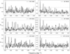 |
Fig. 2 Astrometric PDC periodograms for selected HIPPARCOS binary-star targets from the catalogue of astrometric orbits published by Goldin & Makarov (2007). More information on the targets can be found in Table 1. The dashed vertical lines mark the published orbital frequencies, and the dotted horizontal lines correspond to an FAP level of 10−3. |
3.2 Simulated data
The above results demonstrate that our newly developed peri-odogram is effective for a periodicity detection in HIPPARCOS IAD. The data are given with respect to the catalogue position, and therefore, they are corrected for the proper motion and parallactic motion of the observed star. However, in principle, especially in the presence of some astrophysical periodicity, the correction might not be perfect, and some residual effects of the parallax and the proper motion might still be present. To demonstrate the periodogram suitability in those conditions, we further tested it using a simulation. In addition, the scanning law of the telescope might be affected by the motion of the satellite, and as a result, the scanning angle might not be completely random. We included this effect in our simulation as well.
We randomly drew 35 epochs from a uniform distribution over an interval of 3 yr. We used them to sample the astrometric signature of a Keplerian orbit with a semi-major axis of 5 mas, high eccentricity (e = 0.8), and a period of 100 days. We added to it a circular 5 mas orbit with a period of 365 days and a 60° inclination, to simulate a typical parallax signal, and also a linear trend simulating the effect of a linear 3 mas yr−1 proper motion. We further added white noise to the data at a signal-to-noise ratio of S/N = 75. The astrometric position at each epoch was then translated into the scanning angle and abscissa representation, with the scanning angle following a simulated 60-day satellite rotation period.
Figure 4 shows the results of applying the astrometric PDC to the simulated data described above. A prominent peak indeed appears at the simulated orbital period. An additional peak matching a ~30-day period appears in the periodogram, and it is probably due to interaction between the proper motion and the sampling window function caused by the satellite simulated 60-day rotation period. The residual parallax and proper motion, at the levels we introduced them, do not seem to affect the periodogram ability to detect the orbital period of the system, although a significant peak does appear, as might be expected, around a 1-yr period, probably related to the residual parallactic motion.
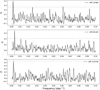 |
Fig. 3 Astrometric PDC periodograms for selected brown dwarf hosting stars. More information on the targets can be found in Table 2. The dashed vertical lines mark the published orbital frequencies, and the dotted horizontal line corresponds to a FAP level of 10−3. |
Details for the brown dwarf hosting stars used for demonstration.
3.3 Comparison with Delisle & Ségransan (2022)
In a recent publication, Delisle & Ségransan (2022) presented an astrometric periodogram based on a linearized Keplerlian model fitted to a set of one-dimensional astrometric measurements. Their approach relies on analytical approximations and is therefore probably superior to ours in terms of its computational cost. They also show that the statistical efficiency of their method degrades slowly as the orbital eccentricity increases, so that a ~10% loss in power is only achieved for e ≳ 0.8. Nevertheless, their approach is still model dependent; for example, it might be suboptimal for detecting extremely eccentric orbits or variability-induced motion. When considering the wide range of variability sources, astrophysical or otherwise, the non-parametric approach presented in this work might prove valuable, and complementary to other techniques.
To demonstrate their method, Delisle & Ségransan (2022) used two systems from the HIPPARCOS database that exhibited astrometric periodicity: HIP 117622 and HIP 12726. We compared the results they obtained in detecting the periodic signals known from the literature to those of the astrometric PDC periodogram. Table 3 shows that the astrometric PDC periodogram successfully detects the known periodicities, with corresponding FAP values comparable to those of Delisle & Ségransan (2022) for the moderately eccentric HIP 117622 (e = 0 25), and an order of magnitude lower for the more eccentric HIP 12726 (e = 0.61).
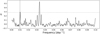 |
Fig. 4 Astrometric PDC periodograms for a simulated system with a 100-day orbital period and a 60-day satellite rotation period. The dashed vertical line marks the simulated orbital frequency, and the dotted horizontal line corresponds to an FAP level of 10−3. An additional peak matching the period of ~30 days appears in the periodogram, and it is probably related to half the satellite rotation period. |
Comparison of the period detection by Delisle & Ségransan (2022) to those performed using the astrometric PDC periodogram for HIP 117622 and HIP 12726.
4 Conclusion
We have presented the astrometric PDC method and demonstrated that it can be used to detect and quantify periodicity in the HIPPARCOS catalogue. It offers a new approach to studying data from scanning astrometry while avoiding complex, model-dependent solutions characterizing the variability, such as Keplerian models. We believe this approach can pave the way to new discoveries and insights.
Considered by many to be HIPPARCOS successor, Gaia was launched in 2014, with its latest data release including more than 1.8 billion stars with an unparalleled high precision (DR3, Gaia Collaboration 2023b). The epoch astrometry data of Gaia is expected to become available to the community as part of the future data release 4 (DR4). Previous data releases have already shown its potential in the classification of stellar multiplicity (Gaia Collaboration 2023a; Halbwachs et al. 2023), and also in the detection of substellar and planetary-mass companions (Holl et al. 2023b). Therefore, we expect our periodogram to be useful for the analysis of the Gaia astrometric data, potentially discovering signals that cannot be identified using standard analysis methods.
In a recent paper (Binnenfeld et al. 2022), we have introduced the partial phase distance correlation periodograms, which allow accounting for nuisance parameters in order to eliminate spurious peaks related to it. In the case of one-dimensional astrometry, the angle θ describing the RGC orientation may be considered a nuisance because it is determined arbitrarily by the satellite orbit and is not related to the examined astrophysi-cal phenomenon (see Holl et al. 2023a). Therefore, we plan to explore reducing its effect using the partial distance correlation periodograms.
Using HIPPARCOS photometry as a nuisance variable to the astrometry may be informative as well. It might help in distinguishing orbital movement from luminosity variability in the case of VIMs. Gaia DR4 will also include various other types of epoch data, such as RVs and photometry in different bands, which we may be able to use in a similar way.
HIPPARCOS data and their astrometric solutions were extensively researched in search of stellar multiplicity, and also for orbital companions such as brown dwarfs and massive planets (e.g. Mazeh et al. 1999; Zucker & Mazeh 2000, 2001; Sozzetti & Desidera 2010; Snellen & Brown 2018). Nevertheless, we believe that due to the unique qualities of our new method, using it to carefully analyse the HIPPARCOS catalogue in its entirety can potentially reveal many new astrometric orbits, especially those of high eccentricity.
Another potential context in which our newly developed tool can contribute significantly is the Nancy Grace Roman Space Telescope (NGRST, known before as WFIRST; Spergel et al. 2013). It is currently expected to launch by 2027.
We provide our Python implementation of the periodogram in the form of a public GitHub repository1.
Acknowledgements
We thank the anonymous referee for their wise comments that helped to improve the manuscript. This research was supported by the Ministry of Innovation, Science & Technology, Israel (grant 3-18143). The research of S.S. is supported by a Benoziyo prize postdoctoral fellowship. The analyses done for this paper made use of the code packages: NumPy (Harris et al. 2020), SciPy (Virtanen et al. 2020) and SPARTA (Shahaf et al. 2020).
References
- Binnenfeld, A., Shahaf, S., & Zucker, S. 2020, A&A, 642, A146 [NASA ADS] [CrossRef] [EDP Sciences] [Google Scholar]
- Binnenfeld, A., Shahaf, S., Anderson, R. I., & Zucker, S. 2022, A&A, 659, A189 [NASA ADS] [CrossRef] [EDP Sciences] [Google Scholar]
- Delisle, J.-B., & Ségransan, D. 2022, A&A, 667, A172 [NASA ADS] [CrossRef] [EDP Sciences] [Google Scholar]
- ESA 1997, The Hipparcos and Tycho Catalogues, ESA SP-1200 (Noordwijk: ESA) [Google Scholar]
- Gaia Collaboration (Prusti, T., et al.) 2016, A&A, 595, A1 [NASA ADS] [CrossRef] [EDP Sciences] [Google Scholar]
- Gaia Collaboration (Arenou, F., et al.) 2023a, A&A, 674, A34 [CrossRef] [EDP Sciences] [Google Scholar]
- Gaia Collaboration (Vallenari, A., et al.) 2023b, A&A, 674, A1 [NASA ADS] [CrossRef] [EDP Sciences] [Google Scholar]
- Goldin, A., & Makarov, V. V. 2007, ApJS, 173, 137 [NASA ADS] [CrossRef] [Google Scholar]
- Halbwachs, J.-L. 2009, MNRAS, 394, 1075 [CrossRef] [Google Scholar]
- Halbwachs, J. L., Arenou, F., Mayor, M., Udry, S., & Queloz, D. 2000, A&A, 355, 581 [Google Scholar]
- Halbwachs, J.-L., Pourbaix, D., Arenou, F., et al. 2023, A&A, 674, A9 [NASA ADS] [CrossRef] [EDP Sciences] [Google Scholar]
- Harris, C. R., Millman, K. J., van der Walt, S. J., et al. 2020, Nature, 585, 357 [NASA ADS] [CrossRef] [Google Scholar]
- Holl, B., Fabricius, C., Portell, J., et al. 2023a, A&A, 674, A25 [NASA ADS] [CrossRef] [EDP Sciences] [Google Scholar]
- Holl, B., Sozzetti, A., Sahlmann, J., et al. 2023b, A&A, 674, A10 [NASA ADS] [CrossRef] [EDP Sciences] [Google Scholar]
- Kovalevsky, J., Falin, J. L., Pieplu, J. L., et al. 1992, A&A, 258, 7 [NASA ADS] [Google Scholar]
- Lindegren, L., & Bastian, U. 2010, EAS Pub. Ser., 45, 109 [NASA ADS] [CrossRef] [EDP Sciences] [Google Scholar]
- Lindegren, L., Hog, E., van Leeuwen, F., et al. 1992, A&A, 258, 18 [NASA ADS] [Google Scholar]
- Lyons, R. 2013, Ann. Probab., 41, 3284 [CrossRef] [Google Scholar]
- Mazeh, T., Zucker, S., Dalla Torre, A., & van Leeuwen, F. 1999, ApJ, 522, L149 [NASA ADS] [CrossRef] [Google Scholar]
- Perryman, M. A. C., Lindegren, L., Kovalevsky, J., et al. 1997, A&A, 323, L49 [Google Scholar]
- Reffert, S., & Quirrenbach, A. 2011, A&A, 527, A140 [NASA ADS] [CrossRef] [EDP Sciences] [Google Scholar]
- Rizzo, M. L., & Székely, G. J. 2016, Wiley Interdiscip. Rev. Comput. Stat., 8, 27 [CrossRef] [Google Scholar]
- Shahaf, S., Binnenfeld, A., Mazeh, T., & Zucker, S. 2020, Astrophysics Source Code Library, [record ascl:2007.022] [Google Scholar]
- Shen, C., Panda, S., & Vogelstein, J. T. 2022, J. Comput. Graph. Stat., 31, 254 [CrossRef] [Google Scholar]
- Snellen, I., & Brown, A. 2018, Nat. Astron., 2, 883 [NASA ADS] [CrossRef] [Google Scholar]
- Sozzetti, A., & Desidera, S. 2010, A&A, 509, A103 [NASA ADS] [CrossRef] [EDP Sciences] [Google Scholar]
- Spergel, D., Gehrels, N., Breckinridge, J., et al. 2013, arXiv e-prints [arXiv:1305.5422] [Google Scholar]
- Székely, G. J., & Rizzo, M. L. 2013, J. Stat. Plan. Inference, 143, 1249 [CrossRef] [Google Scholar]
- Székely, G. J., & Rizzo, M. L. 2014, Ann. Stat., 42, 2382 [Google Scholar]
- Székely, G. J., Rizzo, M. L., & Bakirov, N. K. 2007, Ann. Stat., 35, 2769 [Google Scholar]
- Tokovinin, A. A., Duquennoy, A., Halbwachs, J. L., & Mayor, M. 1994, A&A, 282, 831 [NASA ADS] [Google Scholar]
- van Leeuwen, F. 2007, A&A, 474, 653 [CrossRef] [EDP Sciences] [Google Scholar]
- van Leeuwen, F., & Evans, D. W. 1998, A&As, 130, 157 [NASA ADS] [CrossRef] [EDP Sciences] [Google Scholar]
- Virtanen, P., Gommers, R., Oliphant, T. E., et al. 2020, Nat. Methods, 17, 261 [Google Scholar]
- Wielen, R. 1996, A&A, 314, 679 [NASA ADS] [Google Scholar]
- Zechmeister, M., & Kürster, M. 2009, A&A, 496, 577 [CrossRef] [EDP Sciences] [Google Scholar]
- Zinger, A. A., Kakosyan, A. V., & Klebanov, L. B. 1992, J. Sov. Math., 59, 914 [CrossRef] [Google Scholar]
- Zucker, S. 2018, MNRAS, 474, L86 [NASA ADS] [CrossRef] [Google Scholar]
- Zucker, S. 2019, MNRAS, 484, L14 [NASA ADS] [CrossRef] [Google Scholar]
- Zucker, S., & Mazeh, T. 2000, ApJ, 531, L67 [NASA ADS] [CrossRef] [Google Scholar]
- Zucker, S., & Mazeh, T. 2001, ApJ, 562, 549 [NASA ADS] [CrossRef] [Google Scholar]
PDC and its extensions, including USuRPER, partial distance correlation periodograms, and the periodogram presented in this work, are all available as part of the SPARTA package (Shahaf et al. 2020), at https://github.com/SPARTA-dev/SPARTA
All Tables
Comparison of the period detection by Delisle & Ségransan (2022) to those performed using the astrometric PDC periodogram for HIP 117622 and HIP 12726.
All Figures
|
Fig. 1 Definition of the abscissa residual v for a single-epoch position (am, δm), with respect to the nominal catalogue position (α0, δ0) and the RGC orientation θ. The actual position of the observed target lies somewhere along the dotted arrowed blue segment. The figure is based on one originally published by van Leeuwen & Evans (1998). |
| In the text | |
|
Fig. 2 Astrometric PDC periodograms for selected HIPPARCOS binary-star targets from the catalogue of astrometric orbits published by Goldin & Makarov (2007). More information on the targets can be found in Table 1. The dashed vertical lines mark the published orbital frequencies, and the dotted horizontal lines correspond to an FAP level of 10−3. |
| In the text | |
|
Fig. 3 Astrometric PDC periodograms for selected brown dwarf hosting stars. More information on the targets can be found in Table 2. The dashed vertical lines mark the published orbital frequencies, and the dotted horizontal line corresponds to a FAP level of 10−3. |
| In the text | |
|
Fig. 4 Astrometric PDC periodograms for a simulated system with a 100-day orbital period and a 60-day satellite rotation period. The dashed vertical line marks the simulated orbital frequency, and the dotted horizontal line corresponds to an FAP level of 10−3. An additional peak matching the period of ~30 days appears in the periodogram, and it is probably related to half the satellite rotation period. |
| In the text | |
Current usage metrics show cumulative count of Article Views (full-text article views including HTML views, PDF and ePub downloads, according to the available data) and Abstracts Views on Vision4Press platform.
Data correspond to usage on the plateform after 2015. The current usage metrics is available 48-96 hours after online publication and is updated daily on week days.
Initial download of the metrics may take a while.