| Issue |
A&A
Volume 668, December 2022
|
|
|---|---|---|
| Article Number | A44 | |
| Number of page(s) | 15 | |
| Section | Interstellar and circumstellar matter | |
| DOI | https://doi.org/10.1051/0004-6361/202243942 | |
| Published online | 02 December 2022 | |
GS 121–05–037: A new Galactic chimney candidate with signs of triggered star formation
Instituto de Astronomía y Física del Espacio (UBA, CONICET),
CC 67, Suc. 28,
1428
Buenos Aires, Argentina
e-mail: lsuad@iafe.uba.ar
Received:
3
May
2022
Accepted:
1
September
2022
Aims. The goal of this study is to analyze the H i supershell GS 121–05–037 and its role in triggering star formation.
Methods. To characterize the supershell, we analyzed the H i 21-cm line and the far-infrared emission distributions. In addition, to study the star formation processes related to GS 121-05-037, we used the Gaia survey, together with spectrophotometric calculations, and derived a method to look for massive OB–type stars.
Results. The H i characterization of GS 121–05–037 shows an expanding structure centered at (l, b) ~ (121°.3, −4°.8) in the velocity range from −47.8 to −25.2km s−1. It is located at 3.2 ± 1.0 kpc from the Sun and has a kinetic energy of Ek = (2.1 ± 1.3) × 1050 erg. GS 121 −05−037 presents, in the H i emission distribution, an open morphology toward the Galactic halo. The analysis of the IR emission reveals the presence of 32 Hii regions seen projected into the borders of GS 121–05–037. A spectrophotometric analysis to look for the ionizing stars of these regions reveals that 12 of them would be located at a similar distance to GS 121–05–037.
Conclusions. The relative location between GS 121–05–037 and the Hii regions, together with their age difference, led us to conclude that the ionizing stars could have been created due to the expansion of the H i supershell. On the other hand, the Hii regions located on the interface of two or more supershells could have originated from the collision of the H i structures. Finally, the open morphology of GS 121 –05–037 toward the halo suggests that this large structure could be a Galactic chimney.
Key words: ISM: bubbles / ISM: kinematics and dynamics / HII regions / stars: formation
© L. A. Suad et al. 2022
 Open Access article, published by EDP Sciences, under the terms of the Creative Commons Attribution License (https://creativecommons.org/licenses/by/4.0), which permits unrestricted use, distribution, and reproduction in any medium, provided the original work is properly cited.
This article is published in open access under the Subscribe-to-Open model. Subscribe to A&A to support open access publication.
1 Introduction
A large number of Galactic neutral hydrogen (H i) supershells (GSs) have been cataloged by several authors using different H i databases and identification techniques (Heiles 1979; McClure-Griffiths et al. 2002; Ehlerová & Palouš 2005, 2013; Suad et al. 2014). These structures are predominantly detected in the H i emission distribution, in a given radial velocity range, as huge shells or arc-like features of enhanced H i emission that surrounds regions of low H i emissivity, most of which present an elliptical shape with dimensions ranging from tens to hundreds of parsecs, and even kiloparsecs.
In particular, Suad et al. (2014, hereafter Paper I) developed a catalog of Galactic H i supershell candidates in the outer part of the Galaxy making use of the Leiden-Argentine-Bonn (LAB) survey (Kalberla et al. 2005) with an angular resolution of 34 arcmin. The GS candidates were identified using a combination of two techniques: a visual inspection and an automatic searching algorithm. The authors cataloged a total of 566 GS candidates, among which 80 present an open part toward high Galactic latitudes, and were then also cataloged as chimney candidates.
Since the origin of these large structures is still a subject of debate, in a recent work, Suad et al. (2019) calculated the kinetic energies of the structures cataloged in I, and obtained values between 1 × 1047 and 3.4 × 1051 erg. These energy values are in a range that could be reached by the action of either stellar winds and/or supernova explosions present in OB associations, considering the efficiency of 20% for the conversion of mechanical stellar wind energy into the kinetic energy of the GSs (Weaver et al. 1977). The dynamical ages of the GSs cataloged in Paper 1 range between (5−50) × 106 yr. Therefore, if the mechanism that generated them was due to the action of massive stars, it is to be expected that these stars could currently be in an evolved stage. For the GSs located at high Galactic latitudes, an alternative mechanism for their creation could be the collision with high-velocity clouds (HVC; Tenorio-Tagle 1981; Suad et al. 2019).
The expansion of the GSs into the interstellar medium (ISM) can lead to the generation of cool, dense, high-column density conditions over large spatial scales that may become gravitation-ally unstable generating regions, along the periphery of the H i structures, where star formation could take place. On the other hand, it has long been suspected that supershells may also trigger the formation of molecular gas (McCray & Kafatos 1987; Elmegreen 1998; Dawson et al. 2008). Finally, the interaction of a shock front with pre-existing dense (molecular) clouds can hit and compress the material, inducing in this way its gravitational instability, bringing about star formation. In this work, we study the supershell identified as GS 121–05–037 in I, and its role in the recent star-forming activity.
2 GS 121–05–037
2.1 H i Emission Distribution
GS 121–05–037 is a large H i structure first cataloged as a supershell candidate in the New Catalog of Galactic H i Supershell Candidates in the outer part of the Galaxy (I). Figure 1 shows the H i emission distribution averaged in the velocity range from −43.3 to −38.1 km s−1, where GS 121–05–037 is clearly seen. The well-defined shell-like structure presents an elliptical morphology, elongated toward lower Galactic latitudes. This feature is open facing the halo with dimensions of ~4° × 8o (Δl × Δb), is centered at (l, b) ~ (121°3, −4°.8), and it is located, assuming the Galactic rotation model of Fich et al. (1989), at 3.2 kpc from the Sun.
The velocity interval where the structure is detected was first estimated in Paper I, inspecting the position-position data cube. Under the assumption of symmetric expansion, an ellipsoidal H i feature with a central velocity V0 and an expansion velocity Vexp should depict, in a position-position diagram, an ellipse-like pattern when observed at different radial velocities. At V0 the structure attains its maximum dimension, while at the extreme velocities, either approaching (Vm = V0 − Vexp) or receding (VM = V0 + Vexp), the structure attains its minimum dimension. They inferred Δ V = ∣VM − Vm∣ = 14.4 kms−1. Based on the now available HI4PI data (HI4PI Collaboration 2016), which have a better angular resolution (16.2 arcmin) than the H i data used in I (34 arcmin), we improved this estimation using velocity-position diagrams.
Figure 2 shows a velocity-latitude H i image along with a cross-cut obtained for b = −5°.09. GS 121–05–037 is clearly detected as a large region showing low emissivity and covering the Galactic latitude range from about −7° to −3° at velocities around −37 km s−1. The plot of the right panel allows us to estimate the velocity range where the cavity is observed. This range is determined by the maximum emission seen at VM = −47.8 km s−1 and the shoulder located at Vm = −25.2 km s−1. The minimum value between these two peaks, observed at ~−37 km s−1, corresponds to the central velocity of the structure (marked with a vertical black line). We then estimated the velocity range as ΔV = ∣VM − Vm∣ = 22.6 km s−1 and an expansion velocity of Vexp = ΔV/2 = 11.3 km s−1.
Then, following the procedure described by Suad et al. (2016), we estimated the amount of atomic mass present in GS 121 –05–037, as well as the kinetic energy stored in it. Assuming solar abundances, we obtained Mt = (1.7 ± 0.9) × 105 M⊙ and Ek = (2.1 ± 1.3) × 1050 erg. Although in this work we are using data with better angular resolution than the one used by Suad et al. (2019), it is worth mentioning that the estimated values of the mass and energy are in good agreement, within the errors, with the values previously obtained.
Additionally, the dynamic age of a supershell can also be estimated. It is defined as tdyn = Reff /Vexp, where  , a and b being the semiaxes of the fitted ellipse delineating the H i supershell (see I). We obtained for GS 121–05–037, Reff = 175 ±28 pc, and a dynamic age of tdyn = 15.2± 3.2Myr.
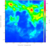 |
Fig. 1 Averaged H i emission distribution of the region of GS 121–05–037 in the velocity range from −43.3 to −38.1 km s−1. Contour levels are superimposed at 20, 30, 40, and 50 K. |
2.2 Infrared Emission
Figure 3 shows the emission distribution at 60 µm, obtained from the Improved Reprocessing of the IRAS Survey (IRIS; Miville-Deschênes & Lagache 2005). An elliptical shell-like structure is also clearly seen at far-infrared wavelengths, showing a good morphological correlation with the emission at 21 cm. Besides the large-scale structure, the presence of several high-intensity regions seen projected onto GS 121–05–037 is clear. Some of these features, indicated by capital letters in Fig. 3, are cataloged as Hii regions in the Sharpless catalog (Sharpless 1959) and/or in the WISE catalog of Galactic Hii Regions (Anderson et al. 2014). Their main parameters, as given in these catalogs, are summarized in Table 1. The information is given as follows:
Columns 1 and 2. designation of the regions in the different catalogs.
Columns 3 (GLON) and 4 (GLAT). Galactic longitude and latitude of the center of the regions in degrees, respectively.
Column 5 (Radius). radius of the regions.
Column 6 (MWSC). stellar clusters detected in the Milky Way global survey of stellar clusters (MWSC; Kharchenko et al. 2013).
Column 7 (VLSR). local standard of rest (LSR) velocity of the radio recombination line or Hα spectroscopic emission in km s−1 .
Column 8 (VmLSR). LSR velocity of the associated molecule (shown in Column 9) in kms-1.
Column 9 (Mol). detected molecule associated with the region.
Column 10 (Dist.). kinematic distance to each region in kpc, estimated by using the Brand (1986) rotation curve model.
Column 11 (Dist.(O.A.). kinematic distance to each region in kpc, estimated by other authors (OA).
Column 12 (Notes). designation associated with each region shown in Fig. 3.
To study the distribution of the dust temperature in the region of GS 121–05–037, we followed the procedure described by Schnee et al. (2005) to construct a dust temperature map from the ratio of the observed fluxes in two IRIS bands, 60 and 100 µm (S60 and S100, respectively). With the assumptions that the dust emission is optically thin at 60 and 100 µm, that Ω60 ~ Ω100, where Ωi is the solid angle subtended at λi by the detector, and with the spectral index of the thermal dust emission β = 2, the temperature can be derived from:

where B(60, T) and B(100, T) are the blackbody Planck function for a temperature T at wavelengths 60 and 100 µm, respectively.
The obtained map is shown in Fig. 4. The presence of warm dust, showing temperatures of about 25−35 K, mixed with the ionized gas regions, is evident. On the other hand, the region located at about (l, b) ~ (119°. 8, −9°. 5) (indicated by a red ellipse in Fig. 4), which is spatially coincident with the lack of emission seen at 21 cm, shows a dust temperature higher by at least 2 K than its surroundings.
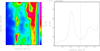 |
Fig. 2 H i emission distribution in the V − l plane. Left panel: radial velocity-latitude H i image averaged in the Galactic longitude range from 120°. 8 to 121°.8. Contour levels are 12, 15, 18, and 21 K. The dashed line indicates the location of the cross-cut shown in the right panel. Right panel: cross-cut at b = −5°. 09 obtained from the left image. The central velocity of GS 121–05–037 is marked as a vertical black line at V = −37 km s−1. |
3 Study of the H ii Regions
As mentioned above, we found 32 ionized regions located at the borders of the supershell. To analyze if they could be related to GS 121 −05−037, it is necessary to verify if they are at the same distance.
Recombination lines and previous works, listed in Table 1, locate ten out of the 32 selected H ii regions at approximately the same distance as the structure. We conducted a study in the direction of the H ii regions, aiming to analyze their stellar components and associate them, or not, with the expanding shell. Since OB-type stars, mainly those earlier than B2, are responsible for the ionization of the H ii regions, our study is centered on the identification of such massive stars. On the one hand, we searched in the literature for OB-type stars confirmed by spectral information and, on the other hand, we conducted a photometric analysis to identify massive star candidates.
To arrange the sample and approach the study of each region, we searched for spatial coincidences between different catalogs. Thus, we found that some of these regions are classified both by WISE and Sharpless catalogs, for example: G118.621−01.329 (Sh2−172), G119.437−00.916 (Sh2−173), G123.155−06.306 (Sh2−184), G123.155−06.306 (Sh2−184), G123.809−01.781 (Sh2−185), and G124.894+00.323 (Sh2−186). Moreover, the size established in the WISE catalog for G123.836−01.762 encloses G123.809−01.781 (Sh2−185), as the same for G124.894+00.323 (Sh2−186), and G124.859+00.323. Furthermore, a search in the MWSC Milky Way global survey of stellar clusters (MWSC; Kharchenko et al. 2013) for previously classified and studied stellar clusters shows that the positions of IC 1590, Mayer 1, BDSB 48, and BDSB 51 are coincident with the H ii regions G123.155−06.306 (Sh2−184), G119.437−00.916 (Sh2−173), G118.621−01.329 (Sh2−172), and G124.894+00.323 (Sh2−186), respectively. At the same time, the stellar cluster FSR 0486 is also superimposed with the H ii regions G118.928−03.337, G118.959−03.321, and G118.977−03.345. The distances listed in the MWSC for IC 1590, Mayer 1, BDSB 51, BDSB 48, and FSR 0486 situate them at 2.4, 1.4, 12.0, 8.0, and 1.8 kpc, respectively.
We studied the stellar components of the H ii regions, adopting the sizes listed in the WISE catalog, except for those superimposed with FSR 0486, in which cases we chose a larger size to include the three WISE regions (see Table 1). In this manner, the sample was reduced to 28 H ii regions, which were then studied individually. We focused on the identification of OB-type stars mainly earlier than B2, within a range of distances consistent with the location of GS 121−05−037. We adopted a distance of 3.2 kpc for GS 121−05−037, with an error of 30% (I). Thus, to study each H ii region, we used first Gaia individual distances and selected only the sources located between 2.2 and 4.2 kpc.
As mentioned before, we conducted this search by dividing the selected sources into two groups. The first group was composed of confirmed OB-type stars, chosen from catalogs and databases that contained spectral type (ST) classifications based on spectral information. For the second group, we conducted an analysis using photometric information. Consequently, these sources were considered as massive star candidates.
In the first case, we examine the SIMBAD database (Wenger et al. 2000), the Galactic O–Star Spectroscopic Survey (GOSSS; Sota et al. 2014), and the Galactic Wolf–Rayet catalog (Rosslowe & Crowther 2015). From these catalogs and databases, we collected confirmed OB-type stars with luminosity class (LC) V in four of the 28 H ii regions. Likewise, we found sources with other spectral types and listed them in Table 2. The confirmed
OB-type stars with LC V were used to perform spectrophotometric calculations. To this end, we computed their color excesses using the Gaia photometric system GBP−GRP, and transformed them to the standard E(B−V) by means of the relative absorption values given by Cardelli et al. (1989). We also calculated their corresponding spectroscopic distances. For this purpose, we used the absolute magnitudes and intrinsic color calibration values from the Gaia survey1 for main sequence (MS) spectral type classifications. For spectral types not included in that survey, we performed a linear interpolation. Based on the calculated color excesses and taking into account high differential reddening and/or possible evolutive effects, we adopted the highest and lowest values of E(B−V) ; E(B−V)M, and E(B−V)m, respectively (see Table 3). These values were extended to the rest of the studied regions, and were used in the following photometric analysis. In all cases and calculations, we considered a normal value for the total to selective extinction ratio RV = 3.1. Table 4 shows the selected spectral types from which we performed the calculations, as well as the results and the distances given by Gaia, for comparison.
In the second case, for selecting massive star candidates, we applied a criterion based on the photometric information provided by the Gaia Early Data Release 3 (eDR3; Gaia Collaboration 2021), the Two Micron All Sky Survey (2MASS; Skrutskie et al. 2006), the individual distances given by Bailer-Jones et al. (2021) from the Gaia EDR3, and the spectrophotometric calculations derived from the confirmed OB-type star with LC V. 2MASS provided IR photometric information in the JHK bands, while Gaia photometric data in the G, G BP, and G RP bands. We constructed the photometric two-color diagram (TCD) in the IR ( J − H) versus (H − K), and color-magnitude diagrams (CMDs) in the IR J versus ( J − H) and optic G versus (GBP−GRP). For the IR 2MASS photometric diagrams, we used the MS reference values given by Koornneef (1983) and Sung et al. (2013). This method is similar to the one already used in previous works (Molina-Lera et al. 2016, 2018, 2019).
We first employed the CMD G versus (GBP−GRP) to select sources within a delimited region, established by placing the MS reference curve at two different positions. For this purpose, we used the previously mentioned bounds, set for distance and color excess: 2.2 kpc and 4.2 kpc, E(B−V)M and E(B−V)m, respectively. It is worth mentioning that E(B−V)M and E(B−V)m were set for each region. The first MS reference curve was placed using the highest values of distance and color excess (4.2 kpc and E(B−V)M), while the second one was set using the lowest values (2.2 kpc and E(B−V)m). Thus, we selected the sources that fall into the delimited region established by these two shifted MS reference curves. Subsequently, for each of these sources, we derived two representative values of their absolute magnitudes in the Gaia G band (MGB and MGb). To accomplish this, we used the upper and lower limits for each individual distance given by Bailer-Jones et al. (2021), combined with E(B−V)M and E(B−V)m established for each H ii region. We then compared the results with those given for known spectral types with LC V, and assigned them their corresponding spectral classification. Finally, we selected the sources for which the result corresponded to a star earlier than B2. Moreover, for verification purposes, we observed their distribution in the IR TCD and CMD. From this analysis, we identified massive star candidates in 12 of the 28 H ii regions.
Figure 5 shows the photometric diagrams, where color circles indicate sources that are situated within 2.2 and 4.2 kpc. The calibration for the MS is represented with a thick blue line, while thinner blue lines in the G versus (GBP−GRP) CMD, on both sides of the MS, enclose the previously mentioned region. Selected massive star candidates are indicated with blue circles and small yellow circles show potential low-mass stars. Discarded sources are shown by green circles, while gray dots show stars with distances lower or higher than 2.2 and 4.2 kpc, respectively. The distribution of the selected massive star candidates is coherent in all photometric diagrams. In Table 2, we present our massive star candidates with their spectral type range, along with the calculated absolutes magnitudes and their previous spectral classification (where available). Furthermore, it can be seen that our spectral type classification is in agreement with previously established spectral information, validating the criteria. In Table 3, we present the main parameters of the 12 regions: the distances, obtained as the average computed from individual distances given by Bailer-Jones et al. (2021) using only the massive star candidates; the excess color and its adopted range; and the designation associated with each region shown in Fig. 3.
As shown in Fig. 5, in the G versus (GBP–GRP) diagrams, the curve that represents E(B−V) is delimited to the right and the left with those of E(B−V)M and E(B−V)m, respectively. Thus, if a higher value were adopted for E(B−V)M and a lower one for E(B−V)m, more sources would be included in the sample, since a larger region would be enclosed in the CMD. On the other hand, the calculated absolute magnitude is a function of the absorption and, therefore, of the adopted color excess value. In this manner, for higher redness values, the calculated absolute magnitude would correspond to that of a brighter source, and thus an earlier spectral type would be assigned. The opposite occurs if the adopted value for the color excess is decreased.
According to our calculations, for a star earlier than O9 to change one subtype, the E(B−V)M or E(B−V)m values should vary by ~0.05−0.1 mag, whereas for spectral types from O9 to B3, a variation of 0.1−0.3 mag is required. Therefore, for any massive star candidate earlier than B2 to be discarded from the sample, it is necessary to modify the adopted value of E(B−V)M or E(B−V)m by more than 0.3 mag. It is worth mentioning that 0.3 mag represents the maximum variation in the adopted E(B−V)M and E(B−V)m values with respect to E(B−V) (see Table 3).
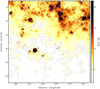 |
Fig. 3 IRIS 60 µm emission distribution in the area of GS 121−05−037. Contour levels at 4, 10, and 15 MJy sr−1 are superimposed. Black and red crosses represent the H ii regions from the WISE catalog of Galactic H ii Regions with and without estimated distances, respectively. Red circles represent the Sharpless H ii regions. |
Hii regions from the WISE and Sharpless catalogs.
Massive star candidates in each of the 12 regions.
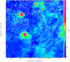 |
Fig. 4 Dust temperature map in the region of GS 121–05–037, derived from the emission at 60 and 100 µm. H i contour levels at 20, 30, 40, and 50 K are superimposed. The red ellipse marks the dust emission region that is seen projected where the H i feature is open toward the halo, and whose temperature is of at least 2 K greater than its surroundings. |
4 Discussion
GS 121–05–037 is a remarkable structure. Its open morphology toward the Galactic halo and the location of several H ii regions seen projected onto the structure make this a striking feature. On the other hand, its expansion velocity, effective radius, and kinetic energy estimates (see Sect. 2.1) are within the values found for hundreds of structures in I and in Suad et al. (2019).
Supershells behind shock fronts experience gravitational instabilities that may lead to the formation of high condensations inside the swept-up gas, and some of them may produce new stars. Observationally, several authors have suggested trigger star formation associated with the expansion of large structures (e.g., Elmegreen 2002; Oey et al. 2005; Paron et al. 2021). This phenomenon has also been detected in other galaxies, as is the case of Holmberg I, where Egorov et al. (2018) detected complexes of ionized gas that reside mainly within dense walls of supershells around OB associations and in walls of giant H i structures.
In the case of the structure studied in this work, we found 32 H ii regions (listed in Table 1) seen projected onto the walls of GS 121–05–037. From Table 1, it can be seen that ten of these regions have a distance or radial velocity estimate similar, within errors, to that of GS 121–05–037. On the other hand, after analyzing the stellar content of the regions (see Sect. 3), we found for 12 of them (listed in Table 3) their associated massive star candidates, located at a distance similar to GS 121–05–037. Among these 12 regions, seven belong to the group of 10 that already had a distance estimate, while five do not. Therefore, of the ten H ii regions whose distances were estimated in other works, we did not find the responsible stars in three of them, G122.002−07.084, G124.037+00.051, and G122.459−00.781, assuming that they are at a distance between 2.2 and 4.2 kpc. An inspection of these three regions revealed that G124.037+00.051 is in fact listed as a young stellar object in The Red MSX Source Survey: The Massive Young Stellar Population of Our Galaxy (Lumsden et al. 2013). As for G122.002−07.084, its distance given in Table 1 (Col. 10) was estimated through its association with an H2O maser that has a measured parallax (Moellenbrock et al 2009) Since distance estimates using parallaxes are more accurate than those obtained by Wenger et al. (2018), given in Table 1 (Col. 11), it is highly probable that this region is located closer than the supershell. Finally, regarding G124.037+00.051, its distance estimate was suggested by Kerton (2002) based on a morphological analysis from which he searched for B1–B5 type stars. Since the region is faint in the radio continuum, it is probable that its ionizing source was later than a B2 star. Another possibility is that the region is actually located at a nearer distance than GS 121−05−037.
If the triggered star formation mechanism is working at the edges of the H i feature, we would expect GS 121 −05−037 to be older than the H ii regions. The fact that we have identified the massive stars responsible for maintaining the ionization in each of the 12 regions shows that these sources have ages lower than a few 106 yr, while the estimated dynamic age of the supershell is much higher, about 15 Myr. This age difference is supported by the fact that we do not detect ionized gas emission associated with the supershell, suggesting that the stars responsible for creating GS 121 −05−037 have already evolved.
The collision of expanding supershells is another well-known mechanism to trigger star formation as it was reproduced in numerical and analytical models by different authors (Chernin et al. 1995; Ntormousi et al. 2011), and observed in our Galaxy, as well as in several nearby galaxies (e.g., Lozinskaya 2002; Dawson et al. 2015; Egorov et al. 2017). In the region of GS 121 −05−037, the presence of several H i supershells, cataloged in Paper I, is conspicuous. Figure 6 shows the H i emission distribution averaged in the velocity range from −43.3 to −38.1 km s−1, where the large H i features located at distances similar to GS 121−05−037 are marked with ellipses. Although two of these structures, GSH 117.8+1.5−35 (Cichowolski et al. 2009) and GS 118+01−44 (Suad et al. 2016), are observed in the same region of the sky, they are present in a different velocity range, as discussed in Suad et al. (2016). On the other hand, the expansion of these two large shells was associated with the origin of the H ii regions Sh2−173 and Sh2−172, indicated as E and G in Fig. 6, respectively (Cichowolski et al. 2009; Suad et al. 2016). The position of the H ii regions that are both located at the same distance as GS 121−05−037 (see Sect. 3) and positioned in the walls of two different supershells are indicated in Fig. 6. The H ii regions named B, C, E, and G are located in the interface between GS 121−05−037, GS 118+01−44, and GSH 117.8+1.5−35, while the H ii regions M and N appear to be between GS 121−05−037 and GS 124−9−43. These findings suggest that the origin of these ionized regions could have been caused by the collision of the supershells.
As mentioned in Sect. 2.1, in the H i emission distribution, GS 121 −05−037 presents an open morphology toward the Galactic halo (see Fig. 1). It is well known that the vertical gas density distribution in a galaxy has a major effect on the evolution of supershells that have sizes exceeding the thickness of a galactic disk, since at these scales the ISM structure is far from homogeneous. In the Milky Way, the warm neutral H i vertical distribution has a long exponential tail with a scale height of about 500 pc (Lockman 1984). Thus, a structure that has reached a size comparable to the H i scale height, could become Rayleigh-Taylor unstable along its polar cap and could eventually break toward the halo. In our case, at the adopted distance of 3.2kpc, the projected ellipse delineating GS 121−05−037 with angular dimensions of 4°.3 × 8°.3 represents a physical size of 240 × 470 pc. Since the supershell has its major dimension perpendicular to the Galactic plane, it is possible that it has already broken toward the halo.
In this scenario, the presence of dust warmer than expected for the more diffuse ISM (Boulanger et al. 1996), located where the H i supershell is open (see Fig. 4), could be a consequence of an ejection phenomenon driven by the effects of multiple supernovae and stellar winds, or could be dust associated with the H i wall of the supershell being broken. Magnetic fields and radiation pressure on dust grains may also play a role in expelling and shaping the dust observed. Dust associated with chimneys was also detected in other spiral galaxies, as in NGC 4217 (Thompson et al. 2004). To better understand the origin of this warm dust structure an exhaustive study is required, which is beyond the scope of this paper.
Main parameters of the 12 H ii regions with associated massive star candidates.
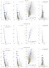 |
Fig. 5 MS curve is represented with a thick blue line . Colored circles indicate the source is situated within 2.2 and 4.2 kpc, while gray dots show stars with distances lower than 2.2 kpc or higher than 4.2 kpc. Thinner blue lines enclose the selected region (see Sect. 3). Massive star candidates are shown with blue circles and labels indicate their previous ST classification. Small yellow circles are potential low-mass stars. Discarded sources are represented by green circles. |
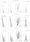 |
Fig. 5 continued. |
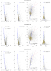 |
Fig. 5 continued. |
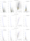 |
Fig. 5 continued. |
Massive stars with spectral type, within the selected distance range, for each of the four regions.
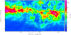 |
Fig. 6 Averaged H i emission distribution of the region of GS 121−05−037 in the velocity range from −43.3 to −38.1 km s−1. Ellipses mark the H i supershells cataloged in I, as well as the supershell GSH 117.8+1.5 (Cichowolski et al. 2009). The black crosses and letters indicate the H ii regions, listed in Table 1, which are located between two supershells. |
5 Summary
We have studied the properties of the H i supershell GS 121−05−037 that was first cataloged in Paper I and analyzed its role in the ISM. From this analysis, we conclude the following:
GS 121−05−037 is located at a distance of 3.2 kpc and has dimensions of 240 × 470 pc. It presents a velocity expansion of Vexp = ΔV/2 = 11.3 km s−1, a total gaseous mass of Mt = (1.7 ± 0.9) × 105 M⊙, a kinetic energy of Ek = (2.1 ± 1.3) × 1050 erg, and a dynamical age of 15 Myr.
From the H i emission distribution, it is clear that GS 121−05−037 is open toward the Galactic halo. This fact, together with the presence of warm dust probably located where the H i feature is open, allows us to conclude that GS 121 −05−037 could be considered as a Galactic chimney.
The infrared emission at 60 µm revealed the presence of 32 H ii regions that are seen projected into the borders of the large H i structure. Using spectrophotometric calculations, we determined that 12 of them could be located at a similar distance to GS 121−05−037. Among these 12 regions, five did not have any previous distance estimation.
The location of the 12 H ii regions on the walls of GS 121−05−037, together with their age difference, led us to the conclusion that the ionizing stars could have been created by the expansion of GS 121−05−037 into the ISM. On the other hand, the collision of H i supershells could be acting as another mechanism inducing star formation.
In summary, all the results presented in this work suggest that GS 121−05−037 is a Galactic H i chimney located in the outer part of the Galaxy. On the other hand, as a consequence of its expansion and/or the collision with other nearby GSs, the formation of new stars could have taken place.
Acknowledgements
This work was supported by CONICET grant PIP 112201701-00604. HI4PI is based on observations with the 100-m telescope of the MPIfR (Max-Planck- Institut für Radioastronomie) at Effelsberg and the Parkes Radio Telescope, which is part of the Australia Telescope and is funded by the Commonwealth of Australia for operation as a National Facility managed by CSIRO. The 2MASS, which is a joint project of the University of Massachusetts and the IPAC/California Institute of Technology, funded by the NASA and the NSF. Data from the ESA mission Gaia, processed by the Gaia DPAC. Funding for the DPAC has been provided by national institutions, in particular the institutions participating in the Gaia Multilateral Agreement. J.A.M.-L. acknowledges support from CONICET grant PIP 112-201701-00055 and PICT 2019-0344.
References
- Anderson, L. D., Bania, T. M., Balser, D. S., et al. 2014, ApJS, 212, 1 [Google Scholar]
- Anderson, L. D., Armentrout, W. P., Johnstone, B. M., et al. 2015, ApJS, 221, 26 [NASA ADS] [CrossRef] [Google Scholar]
- Bailer-Jones, C. A. L., Rybizki, J., Fouesneau, M., Demleitner, M., & Andrae, R. 2021, AJ, 161, 147 [Google Scholar]
- Balser, D. S., Rood, R. T., Bania, T. M., & Anderson, L. D. 2011, ApJ, 738, 27 [NASA ADS] [CrossRef] [Google Scholar]
- Boulanger, F., Abergel, A., Bernard, J.-P., et al. 1996, A&A, 312, 256 [NASA ADS] [Google Scholar]
- Brand, J. 1986, PhD thesis, Leiden Univ., Netherlands [Google Scholar]
- Brand, J., & Blitz, L. 1993, A&A, 275, 67 [NASA ADS] [Google Scholar]
- Cardelli, J. A., Clayton, G. C., & Mathis, J. S. 1989, ApJ, 345, 245 [Google Scholar]
- Chernin, A. D., Efremov, Y. N., & Voinovich, P. A. 1995, MNRAS, 275, 313 [NASA ADS] [CrossRef] [Google Scholar]
- Cichowolski, S., Romero, G. A., Ortega, M. E., Cappa, C. E., & Vasquez, J. 2009, MNRAS, 394, 900 [NASA ADS] [CrossRef] [Google Scholar]
- Dawson, J. R., Mizuno, N., Onishi, T., McClure-Griffiths, N. M., & Fukui, Y. 2008, MNRAS, 387, 31 [NASA ADS] [CrossRef] [Google Scholar]
- Dawson, J. R., Ntormousi, E., Fukui, Y., Hayakawa, T., & Fierlinger, K. 2015, ApJ, 799, 64 [NASA ADS] [CrossRef] [Google Scholar]
- Egorov, O. V., Lozinskaya, T. A., Moiseev, A. V., & Shchekinov, Y. A. 2017, MNRAS, 464, 1833 [NASA ADS] [CrossRef] [Google Scholar]
- Egorov, O. V., Lozinskaya, T. A., Moiseev, A. V., & Smirnov-Pinchukov, G. V. 2018, MNRAS, 478, 3386 [NASA ADS] [CrossRef] [Google Scholar]
- Ehlerová, S., & Palouš, J. 2005, A&A, 437, 101 [NASA ADS] [CrossRef] [EDP Sciences] [Google Scholar]
- Ehlerová, S., & Palouš, J. 2013, A&A, 550, A23 [NASA ADS] [CrossRef] [EDP Sciences] [Google Scholar]
- Elmegreen, B. G. 1998, ASP Conf. Ser., Origins, eds. C. E. Woodward, J. M. Shull, & H. A. Thronson, Jr., 148, 150 [Google Scholar]
- Elmegreen, B. G. 2002, in Extragalactic Star Clusters, eds. D. P. Geisler, E. K. Grebel, & D. Minniti, 207, 390 [NASA ADS] [Google Scholar]
- Fich, M., Blitz, L., & Stark, A. A. 1989, ApJ, 342, 272 [NASA ADS] [CrossRef] [Google Scholar]
- Foster, T., & Brunt, C. M. 2015, AJ, 150, 147 [NASA ADS] [CrossRef] [Google Scholar]
- Gaia Collaboration (Brown, A. G. A., et al.) 2021, A&A, 650, C3 [EDP Sciences] [Google Scholar]
- Heiles, C. 1979, ApJ, 229, 533 [NASA ADS] [CrossRef] [Google Scholar]
- HI4PI Collaboration (Ben Bekhti, et al.) 2016, A&A, 594, A116 [NASA ADS] [CrossRef] [EDP Sciences] [Google Scholar]
- Kalberla, P. M. W., Burton, W. B., Hartmann, D., et al. 2005, A&A, 440, 775 [NASA ADS] [CrossRef] [EDP Sciences] [Google Scholar]
- Kerton, C. R. 2002, AJ, 124, 3449 [NASA ADS] [CrossRef] [Google Scholar]
- Kharchenko, N. V., Piskunov, A. E., Schilbach, E., Röser, S., & Scholz, R.-D. 2013, A&A, 558, A53 [NASA ADS] [CrossRef] [EDP Sciences] [Google Scholar]
- Koornneef, J. 1983, A&As, 51, 489 [NASA ADS] [Google Scholar]
- Lockman, F. J. 1984, ApJ, 283, 90 [NASA ADS] [CrossRef] [Google Scholar]
- Lozinskaya, T. A. 2002, A&A Trans., 21, 223 [NASA ADS] [Google Scholar]
- Lumsden, S. L., Hoare, M. G., Urquhart, J. S., et al. 2013, ApJS, 208, 11 [Google Scholar]
- McClure-Griffiths, N. M., Dickey, J. M., Gaensler, B. M., & Green, A. J. 2002, ApJ, 578, 176 [NASA ADS] [CrossRef] [Google Scholar]
- McCray, R., & Kafatos, M. 1987, ApJ, 317, 190 [NASA ADS] [CrossRef] [Google Scholar]
- Miville-Deschênes, M.-A., & Lagache, G. 2005, ApJS, 157, 302 [Google Scholar]
- Moellenbrock, G. A., Claussen, M. J., & Goss, W. M. 2009, ApJ, 694, 192 [NASA ADS] [CrossRef] [Google Scholar]
- Molina-Lera, J. A., Baume, G., Gamen, R., Costa, E., & Carraro, G. 2016, A&A, 592, A149 [NASA ADS] [CrossRef] [EDP Sciences] [Google Scholar]
- Molina Lera, J. A., Baume, G., & Gamen, R. 2018, MNRAS, 480, 2386 [NASA ADS] [CrossRef] [Google Scholar]
- Molina Lera, J. A., Baume, G., & Gamen, R. 2019, MNRAS, 488, 2158 [NASA ADS] [CrossRef] [Google Scholar]
- Ntormousi, E., Burkert, A., Fierlinger, K., & Heitsch, F. 2011, ApJ, 731, 13 [NASA ADS] [CrossRef] [Google Scholar]
- Oey, M. S., Watson, A. M., Kern, K., & Walth, G. L. 2005, AJ, 129, 393 [NASA ADS] [CrossRef] [Google Scholar]
- Paron, S., Granada, A., & Areal, M. B. 2021, MNRAS, 505, 4813 [NASA ADS] [CrossRef] [Google Scholar]
- Reid, M. J., Menten, K. M., Brunthaler, A., et al. 2014, ApJ, 783, 130 [Google Scholar]
- Rosslowe, C. K., & Crowther, P. A. 2015, MNRAS, 447, 2322 [NASA ADS] [CrossRef] [Google Scholar]
- Russeil, D., Adami, C., & Georgelin, Y. M. 2007, A&A, 470, 161 [NASA ADS] [CrossRef] [EDP Sciences] [Google Scholar]
- Sabbadin, F., Minello, S., & Bianchini, A. 1977, A&A, 60, 147 [NASA ADS] [Google Scholar]
- Schnee, S. L., Ridge, N. A., Goodman, A. A., & Li, J. G. 2005, ApJ, 634, 442 [NASA ADS] [CrossRef] [Google Scholar]
- Sharpless, S. 1959, ApJS, 4, 257 [Google Scholar]
- Skrutskie, M. F., Cutri, R. M., Stiening, R., et al. 2006, AJ, 131, 1163 [NASA ADS] [CrossRef] [Google Scholar]
- Sota, A., Maíz Apellániz, J., Morrell, N., et al. 2014, ApJS, 211, 10 [NASA ADS] [CrossRef] [Google Scholar]
- Suad, L. A., Caiafa, C. F., Arnal, E. M., & Cichowolski, S. 2014, A&A, 564, A116 (Paper I) [NASA ADS] [CrossRef] [EDP Sciences] [Google Scholar]
- Suad, L. A., Cichowolski, S., Noriega-Crespo, A., et al. 2016, A&A, 585, A154 [NASA ADS] [CrossRef] [EDP Sciences] [Google Scholar]
- Suad, L. A., Caiafa, C. F., Cichowolski, S., & Arnal, E. M. 2019, A&A, 624, A43 [NASA ADS] [CrossRef] [EDP Sciences] [Google Scholar]
- Sung, H., Lim, B., Bessell, M. S., et al. 2013, J. Korean Astron. Soc., 46, 103 [NASA ADS] [CrossRef] [Google Scholar]
- Tenorio-Tagle, G. 1981, A&A, 94, 338 [NASA ADS] [Google Scholar]
- Thompson, M. A., White, G. J., Morgan, L. K., et al. 2004, A&A, 414, 1017 [NASA ADS] [CrossRef] [EDP Sciences] [Google Scholar]
- Weaver, R., McCray, R., Castor, J., Shapiro, P., & Moore, R. 1977, ApJ, 218, 377 [Google Scholar]
- Wenger, M., Ochsenbein, F., Egret, D., et al. 2000, A&As, 143, 9 [NASA ADS] [CrossRef] [EDP Sciences] [Google Scholar]
- Wenger, T. V., Balser, D. S., Anderson, L. D., & Bania, T. M. 2018, ApJ, 856, 52 [Google Scholar]
All Tables
Massive stars with spectral type, within the selected distance range, for each of the four regions.
All Figures
|
Fig. 1 Averaged H i emission distribution of the region of GS 121–05–037 in the velocity range from −43.3 to −38.1 km s−1. Contour levels are superimposed at 20, 30, 40, and 50 K. |
| In the text | |
|
Fig. 2 H i emission distribution in the V − l plane. Left panel: radial velocity-latitude H i image averaged in the Galactic longitude range from 120°. 8 to 121°.8. Contour levels are 12, 15, 18, and 21 K. The dashed line indicates the location of the cross-cut shown in the right panel. Right panel: cross-cut at b = −5°. 09 obtained from the left image. The central velocity of GS 121–05–037 is marked as a vertical black line at V = −37 km s−1. |
| In the text | |
|
Fig. 3 IRIS 60 µm emission distribution in the area of GS 121−05−037. Contour levels at 4, 10, and 15 MJy sr−1 are superimposed. Black and red crosses represent the H ii regions from the WISE catalog of Galactic H ii Regions with and without estimated distances, respectively. Red circles represent the Sharpless H ii regions. |
| In the text | |
|
Fig. 4 Dust temperature map in the region of GS 121–05–037, derived from the emission at 60 and 100 µm. H i contour levels at 20, 30, 40, and 50 K are superimposed. The red ellipse marks the dust emission region that is seen projected where the H i feature is open toward the halo, and whose temperature is of at least 2 K greater than its surroundings. |
| In the text | |
|
Fig. 5 MS curve is represented with a thick blue line . Colored circles indicate the source is situated within 2.2 and 4.2 kpc, while gray dots show stars with distances lower than 2.2 kpc or higher than 4.2 kpc. Thinner blue lines enclose the selected region (see Sect. 3). Massive star candidates are shown with blue circles and labels indicate their previous ST classification. Small yellow circles are potential low-mass stars. Discarded sources are represented by green circles. |
| In the text | |
|
Fig. 5 continued. |
| In the text | |
|
Fig. 5 continued. |
| In the text | |
|
Fig. 5 continued. |
| In the text | |
|
Fig. 6 Averaged H i emission distribution of the region of GS 121−05−037 in the velocity range from −43.3 to −38.1 km s−1. Ellipses mark the H i supershells cataloged in I, as well as the supershell GSH 117.8+1.5 (Cichowolski et al. 2009). The black crosses and letters indicate the H ii regions, listed in Table 1, which are located between two supershells. |
| In the text | |
Current usage metrics show cumulative count of Article Views (full-text article views including HTML views, PDF and ePub downloads, according to the available data) and Abstracts Views on Vision4Press platform.
Data correspond to usage on the plateform after 2015. The current usage metrics is available 48-96 hours after online publication and is updated daily on week days.
Initial download of the metrics may take a while.