| Issue |
A&A
Volume 666, October 2022
|
|
|---|---|---|
| Article Number | A105 | |
| Number of page(s) | 13 | |
| Section | Interstellar and circumstellar matter | |
| DOI | https://doi.org/10.1051/0004-6361/202243908 | |
| Published online | 14 October 2022 | |
Studying a precessing jet of a massive young stellar object within a chemically rich region
1
CONICET – Universidad de Buenos Aires. Instituto de Astronomía y Física del Espacio, Ciudad Universitaria,
Buenos Aires, Argentina
e-mail: sparon@iafe.uba.ar
2
Observatorio Astronómico, Universidad Nacional de Córdoba,
Laprida 854,
X5000BGR
Córdoba, Argentina
3
Isaac Newton Group of Telescopes,
38700
La Palma, Spain
4
Instituto de Astrofísica de Canarias; Departamento de Astrofísica, Universidad de La Laguna,
La Laguna, Tenerife
E-38200, Spain
5
Instituto de Matemática, Física y Estadística, Universidad de Las Américas,
Avenida República 71,
Santiago, Chile
6
Facultad de Ingeniería, Universidad del Desarrollo,
Avenida la Plaza 680,
Santiago, Chile
Received:
29
April
2022
Accepted:
4
August
2022
Aims. In addition to the large surveys and catalogs of massive young stellar objects (MYSOs) and outflows, dedicated studies are needed of particular sources in which high angular observations, mainly at near-IR and (sub)millimeter wavelengths, are analyzed in depth, to shed light on the processes involved in the formation of massive stars. The galactic source G079.1272+02.2782 is a MYSO at a distance of about 1.4 kpc that appears in several catalogs, and is hereafter referred to as MYSO G79. It is an ideal source to carry out this kind of study because of its relatively close distance and the intriguing structures that the source shows at near-IR wavelengths.
Methods. Near-IR integral field spectroscopic observations were carried out using NIFS at Gemini North. The spectral and angular resolutions, about 2.4–4.0 Å, and 0.″15–0.″22, allow us to perform a detailed study of the source and its southern jet, resolving structures with sizes between 200 and 300 au. As a complement, millimeter data retrieved from the James Clerk Maxwell Telescope and the IRAM 30 m telescope databases were analyzed to study the molecular gas around the MYSO on a larger spatial scale.
Results. The detailed analysis of a jet extending southward from MYSO G79 shows corkscrew-like structures at 2.2 μm continuum, strongly suggesting that the jet is precessing. The jet velocity is estimated at between 30 and 43 km s−1 and its kinematics indicates that it is blueshifted, that the jet is coming to us along the line of sight. We suggest that the precession may be produced by the gravitational tidal effects generated in a probable binary system, and we estimate a jet precession period of about 103 yr, indicating a slow-precessing jet, which is in agreement with the observed helical features. An exhaustive analysis of H2 lines at the near-IR band along the jet allows us to investigate in detail a bow shock produced by this jet. We find that this bow shock is indeed generated by a C-type shock and it is observed coming to us, at an inclination angle, along the line of sight. This is confirmed by the analysis of molecular outflows on a larger spatial scale. A brief analysis of several molecular species at millimeter wavelengths indicates a complex chemistry developing at the external layers of the molecular clump in which MYSO G79 is embedded. We note that we are presenting interesting observational evidence that can give support to theoretical models of bow shocks and precessing jets.
Key words: stars: formation / stars: protostars / ISM: jets and outflows / ISM: molecules
© S. Paron et al. 2022
 Open Access article, published by EDP Sciences, under the terms of the Creative Commons Attribution License (https://creativecommons.org/licenses/by/4.0), which permits unrestricted use, distribution, and reproduction in any medium, provided the original work is properly cited.
This article is published in open access under the Subscribe-to-Open model. Subscribe to A&A to support open access publication.
1 Introduction
It is known that massive young stellar objects (MYSOs) are short lived and they form deeply embedded in dense molecular clumps. In general, the relevant phases of massive stars formation are very difficult to be observed, and hence they remain in the darkness and prevent our complete knowledge about star formation. However, theoretical and observational studies support the idea that MYSOs might be born as a scaled-up version of their low-mass counterparts (e.g., Beuther et al. 2007; Tan et al. 2014; Frost et al. 2019).
As in low-mass YSOs, structures in Keplerian rotation have been discovered in massive protostars and they were associated with accretion discs or toroids (e.g., Beltrán et al. 2016). Additionally, jets related to MYSOs were also discovered (McLeod et al. 2018), and powerful molecular outflows related to cores containing massive protostars were extensively surveyed (Davis et al. 2004; Caratti o Garatti et al. 2015; Maud et al. 2015b and references therein).
In order to probe gaseous disks, cavities generated by jets, and shocked and ionized gas at the close surroundings of massive protostars we need to observe at near-IR bands. For instance, the analysis of the CO overtone bandheads, H2 and Brγ emission lines, in addition to the continuum emission at these wavelengths, is very useful to carry out deep studies of such structures and/or processes related to massive star formation (Hoffmeister et al. 2006; Martins et al. 2010; Fedriani et al. 2020). The analysis of the H2 lines and the ratios among them is useful in discerning the excitation mechanisms responsible for the emission of this molecule, which can be excited due to collisions produced by shock fronts or fluorescence excitation by nonionizing UV photons in the Lyman-Werner band (912–1108 Å). These mechanisms can be distinguished since they preferentially populate different levels producing different line ratios (Davis et al. 2003; Martín-Hernández et al. 2008). Moreover, using spectroscopy at near-IR bands, it is possible to trace the jet kinematics, to estimate radial velocities, and/or to study velocity fields. In addition, the near-IR imaging allows us to indirectly analyze tidal forces and torques that might be visible as three-dimensional effects in the jet structure and jet propagation. There are theoretical models and observational evidence that indicate nonaxisymmetric features like jet precession or curved ballistic motion of the jet suggesting that the jet source is part of a binary system or even a multiple system (see Sheikhnezami & Fendt 2022, and references therein).
Currently there are useful surveys of MYSOs, molecular outflows, and extended near-IR H2 emission related to high-mass young stars (Lumsden et al. 2013; Navarete et al. 2015; Caratti o Garatti et al. 2015; Maud et al. 2015a,b; Yang et al. 2018). These surveys provide large and homogeneous samples of sources that allow us to select particular objects to perform dedicated observations for deeper and more detailed studies of individual objects. Studies of particular sources (see, e.g., Gredel 2006; Fedriani et al. 2019, 2020 and Areal et al. 2020), in which the observations, mainly at near-IR and (sub)millimeter wavelengths, are analyzed in depth, are extremely useful to shed light on the formation processes of MYSOs.
In this work we investigate MYSO G079.1272+02.2782 (hereafter MYSO G79) and its close surroundings using near-IR integral field spectroscopic observations, which allows us to obtain detailed information from both spectra and photometry. Additionally, using millimeter data retrieved from the James Clerk Maxwell Telescope (JCMT) and the IRAM 30 m telecope databases, we analyze the molecular gas around MYSO G79 at a larger spatial scale with the aim of complementing the near-IR results.
MYSO G79, related to IRAS 20216+4107, is an interesting object located at a distance of about 1.4 kpc, quite close for a MYSO, that presents NH3 maser emission (Urquhart et al. 2011). This source is included in the distance-limited sample of massive molecular outflows studied by Maud et al. (2015b) through the emission of the CO J = 3–2 line, and its outflows have a total mass of about 8 M⊙. Navarete et al. (2015) detected extended H2 emission in the near-IR toward this object. This source is cataloged as MHO3476 in the UKIRT Widefield Infrared Survey for H2 (UWISH2), a survey of YSO jets in the Galactic plane, particularly toward the Galactic region Cygnus-X (Makin & Froebrich 2018). According to the catalog, MHO3476 presents only one H2 outflow lobe whose emission is observed as a collection of knots. A single spectrum in the near-IR of MYSO G79 reveals only a H2 line (1–0 S(1) at 2.12 μm) and some upper values for other lines (Cooper et al. 2013). This source, also cataloged as a high-mass protostellar object (HMPO; Sridharan et al. 2002), was observed, among 59 high-mass star-forming regions, using the IRAM 30 m telescope at bands 86–94GHz, 217–221GHz, and 241–245 GHz (Gerner et al. 2014). Several molecular lines, such as H13CO+, HN13C, HCN, HCO+ J = 1–0 among many others, were observed toward MYSO G79. These molecules were used by the authors to study the chemical evolution in the early phases of massive star formation in the analyzed sample.
Figure 1 displays a RGB image of the JHKs-band emission obtained from the UKIRT Infrared Deep Sky Survey (UKIDSS). Several arc-like features appears extending from the central object (indicated as MYSO G79 in the figure) to the south, suggesting a cavity carved out by a precessing jet or a helical flow (see discussion below). Toward the north some extended near-IR emission also appears, and an unrelated point-like source; its different color should be noted, not reddened, indicating that this source is not as deeply embedded as MYSO G79. Taking into account the relatively close distance; the high galactic latitude, which avoids confusion due to the emission and absorption of material along the galactic plane; and the information published in several catalogs and surveys, MYSO G79 is an ideal source to carry out a dedicated study with high angular and spectral resolution and high sensitivity in the near-IR using integral field spectroscopy. We focus our study on the central source and the southern extended emission.
The paper is organized as follows. Section 2 describes the near-IR observations and the data reduction. Section 3 presents the results obtained from the analysis of the near-IR data. In Sect. 4 these results are discussed together with a discussion regarding the molecular gas and chemistry on a larger spatial scale. Finally, in Sect. 5 we present our concluding remarks.
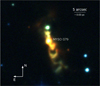 |
Fig. 1 Three-color image with the JHKs emission extracted from the UKIRT Infrared Deep Sky Survey (UKIDSS) presented in blue, green, and red, respectively. The bar of 5 arcsec represents a size of ~0.03 pc at the assumed distance of 1.4 kpc. |
2 Observations and data reduction
Near-IR integral field spectroscopic observations were carried out using the Near-infrared Integral Field Spectrograph (NIFS, McGregor et al. 2003) located at Gemini North during the first semester of 2019 (project: GN-2019A-Q-108-47). NIFS was used together with the Gemini North Adaptive Optics facility ALTAIR with a natural guide star (NGS). The NGS chosen was TYC 3160-1037-1, a star of unknown spectral type at RA = 20:23:24.12, Dec = +41:17:16.5. With UCAC4 mag V = 11.35 (R = 11.47) this NGS is well within the V-band limit for full correction regime. ALTAIR was used with field lens IN to improve the Strehl ratios and image quality as the NGS is farther than 5 arcsec from centers of all the fields.
The K_G5605 grating (central wavelength 2.20 μm, spectral range 1.99–2.40 μm, spectral resolution 5290) together with the HK_G0603 filter (central wavelength 2.16 μm, spectral range 1.57–2.75 μm) were used to observe five fields that cover the G79 MYSO compact object and the southern arc-like features. The field centers and position angles were chosen to enclose the main structures as seeing in the UKIDSS image (see Fig. 2) in compromise with the separation imposed by the guide star. The position centers of the observed fields, the integration times, the position angle (PA), and the separation between the NGS and the field centers are presented in Table 1.
The observations followed the Object-Sky dither sequence, with off-source sky positions, and spectra centered at 2.2 μm. The spectral range is 2.009–2.435 μm. The spectral resolution ranges from 2.4 to 4.0 Å, as determined from the full width at half maximum (FWHM) measurement of the ArXe lamp lines used to calibrate the wavelength of the spectra. This results in velocity resolutions in the range 33–55 km s−1. The error on the determination of the radial velocities depends on the signal-to-noise ratio (S/N) of the measured lines (see Sect. 3.1). The angular resolution is in the range of 0.″15–0.″22, derived from the FWHM of the flux distribution of telluric standard stars, which corresponds to 0.0010–0.0015 pc (206–310 au) at the distance of G79. As there are no point sources in the fields, it is not possible to measure the final correction made by the ALTAIR system. In any case, the distances reported in Table 1 between the NGS and the fields, and the magnitude of the NGS, both within the expected limits to obtain a close-to-full correction, indicate that the spatial resolution achieved in the fields corresponds to the range mentioned above.
The standard NIFS tasks included in the Gemini IRAF package v1.141 were used for data reduction. The procedure included image trimming, flat-fielding, sky subtraction, wavelength calibration, and S-distortion correction. The telluric correction of the fields was performed by observing two telluric standards: HIP 102074 for Fields 1-4 and HIP 103159 for Field 5. The telluric correction process included fitting the hydrogen absorption lines of the stellar spectrum and fitting a synthetic blackbody spectrum to recover the correct shape of the spectral distribution. These telluric stars were also used to flux calibrate the datacubes. Finally, datacubes were created for each field with a field of view (FoV) of 3″ × 3″ and an angular sampling of 0.″05 × 0.″05. For the analysis of the datacubes we used the code IFSCUBE2 (Ruschel-Dutra et al. 2021). For each emission line detected in the datacube, this analysis consists in fitting a continuum to each spaxel and then fitting a Gaussian function to the emission line. This way we obtained the flux, the FWHM, the central wavelength, and the continuum value corresponding to each spaxel in the field. With this information we were able to construct maps of the spatial distribution of these parameters.
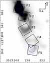 |
Fig. 2 Ks-band emission extracted from the UKIRT Infrared Deep Sky Survey (UKIDSS) toward MYSO G79. The numbered boxes are the 3″ × 3″ fields observed using NIFS at Gemini. The dashed blue circles are the regions from which the spectra presented below were extracted. |
Observed fields using NIFS+ALTAIR at Gemini North.
3 Results
In this section, we present the spectra with the line identification, continuum maps, and line emission maps with continuum subtracted of each observed field. To facilitate the interpretation of the maps, the figures are presented with the same inclination (i.e., PA with respect to the equatorial coordinates) as the fields shown in Fig. 2.
3.1 Spectra
In what follows, we present the spectra obtained toward each field in which atomic and molecular lines appear. After a careful inspection of each datacube we find that these lines appear in Fields 1, 2, and 5. Fields 3 and 4 lack emission lines. The blue dashed circles displayed in Fig. 2 represent the regions in these fields from which the spectra presented below were extracted. These are the regions in which the emission lines are clearly present within the observed field.
Figure 3 displays the spectrum in the whole observed wavelength range obtained toward Field 1 from a circular region (radius about 078; see Fig. 2) at the position in which emission lines appear (see the maps Sect. 3.2). By inspecting the whole Field 2 we found only a strong emission line of H2 1–0 S(1) almost at the upper left corner of the observed field (see the circular region of 0.″6 in radius in Fig. 2). This region also presents a Brγ marginal emission. Figure 4 shows the spectrum obtained from such a region. Finally, Field 5 presents very weak continuum emission and it is the richest field among the five observed in H2 lines. Figure 5 displays a spectrum obtained toward a region of about 2″ in diameter lying almost at the center of the field (see Fig. 2), in which all detected H2 lines are indicated.
From the H2 1–0 S(1) emission line in Field 5, we obtain a radial velocity (vLSR) for the gas of about −31 km s−1. This line was chosen for the radial velocity determination for two reasons. It has a S/N of ~174 on the peak emission and ~10 in the lowest part of the map, and also because is near the central wavelength of the spectra, which ensures that the wavelength calibration is optimal compared to transitions located at the redder end of the spectrum. According to our empiric experience, this high S/N allows us to obtain radial velocities with a precision of 1/10 of the spectral resolution. The errors for the reported radial velocities, considering the fitting error and the wavelength calibration, are in the range 10–15 km s−1. To estimate these errors we considered the uncertainty in the continuum fitting and the variations of different lines along the spectra when available.
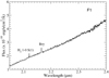 |
Fig. 3 Spectrum obtained toward a region of about 1.″6 in diameter (see Fig. 2) in which the lines appear in Field 1. |
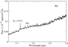 |
Fig. 4 Spectrum obtained from a region of about 1.″2 in diameter toward the upper left corner of Field 2 (see Fig. 2). |
3.2 Maps
In what follows, we present the continuum and the emission line (continuum subtracted) maps from each field.
Figure 6 displays the 2.2 μm continuum map, and the Brγ and H2 1–0 S(1) continuum subtracted emission line maps in Field 1. This field, in which the protostar (understood as the compact object) lies, presents only emission of Brγ and H2 1–0 S(1).
Field 2 possibly marks the beginning of a jet driven by the source located at Field 1 or a cavity produced by such a jet, that extends toward the southwest (see Fig. 1). The only significant emission line that appears in this field is H2 1–0 S(1). Figure 7 displays the 2.2 μm continuum map and the mentioned H2 line map with the continuum subtracted.
For Fields 3 and 4, we present only the continuum maps (Figs. 8 and 9). As mentioned above, no line above the noise level appears in such fields.
Field 5 likely marks the end of the jet driven by MYSO G79 or the jet cavity. Figures 10 and 11 present the 2.2 μm continuum map and the H2 line maps with the continuum subtracted of this field. The molecular emission shows an almost circular morphology uncorrelated with the morphology of the continuum emission. This feature has a radius of about 1.″1 (~1500 au at the distance of 1.4 kpc). Finally, Fig. 12 displays the intensity-weighted mean velocity (moment 1) of the H2 1–0 S(1) line in Field 5. As mentioned above, the central velocity of the line is υLSR ~ −31 km s−1.
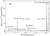 |
Fig. 5 Spectrum obtained from a region of about 2″ in diameter toward almost the center of Field 5 (see Fig. 2). |
3.3 Line ratios in Fields 1 and 5
Even though line ratios cannot be used as the sole discriminant of excitation mechanisms of the gas (Burton 1992), together with the analysis of the context in which the lines arise they can be used to have a good idea about such mechanisms.
In Field 1, given that only one H2 line appears, we can make a comparison between the molecular and atomic hydrogen emission through the H2 1–0 S(1)/Brγ line ratio. This kind of molecular-to-atomic line ratio is commonly used to distinguish between various excitation mechanisms (Hatch et al. 2005; Chen et al. 2015). Figure 13 displays a map of such a ratio, where values above 4σ in both lines were used. The average value of the H2 1–0 S(1)/Brγ line ratio is 0.6, which is discussed in Sect. 4.1.
The richness of H2 lines and the good quality of the data in Field 5 allow us to perform a line ratio study with the aim of establishing the nature of the molecular emission that presents such curious morphology in the context of a likely end of a jet. Following Martín-Hernández et al. (2008) and Chen et al. (2015), we present the H2 1–0/2–1 S(1), 1–0 S(1)/3–2 S(3), and 1–0 Q(1)/1–0 S(1) ratios to distinguish between collisional and radiative H2 excitation (see Fig. 14). It is important to be cautious with unreal low values in the H2 2–1 S(1), 3–2 S(3), and 1–0 Q(1) emissions that yield artificially high values in the corresponding ratios. Thus, only values above 5σ for such emissions were used. The average values along the whole field of the presented ratios are 11, 50, and 0.74, respectively, and the value ranges (min.−max.) of each ratio are 6.6–16.5, 17.8–94.8, and 0.65–0.87. The meaning of these values is discussed in Sect. 4.3.
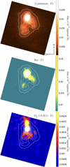 |
Fig. 6 Maps obtained toward Field 1. The 2.2 μm continuum map (top) is displayed in color scale with contours that are superimposed for comparison in the Brγ (middle) and H2 1–0 S(1) (bottom) line emission maps (continuum subtracted). The background rms is ~0.15, 2.97, and 0.65 × 10⁻²³ erg s−1 cm−2Å−1 for the continuum, the Brγ, and the H2 maps respectively. |
4 Discussion
As presented in Fig. 1, at near-IR bands MYSO G79 presents a striking morphology with knots and arcs extending southward from the compact object (i.e., the massive protostar). Thus, this is an interesting case to study in great detail the physical consequences of such a jet in the MYSO close surroundings. The Gemini NIFS data allow us to perform a kinematical and a detailed qualitatively morphological study of the continuum and emission lines, and from the evaluation of line ratios we can discern the line excitation mechanisms. In what follows, we discuss the main results in each observed field, and we finish with a comprehensive view of the possible dynamics of the jet trying to explain such a complex morphology.
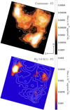 |
Fig. 7 Maps obtained toward Field 2. The 2.2 μm continuum map (top) is displayed in color scale with contours that are superimposed for comparison in the continuum subtracted H2 1–0 S(1) line emission map (bottom). The background rms is ~2.0 and 20 × 10−23 erg s−1 cm−2 Å−1 for the continuum and the H2 maps respectively. |
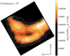 |
Fig. 8 Map of the 2.2 μm continuum obtained toward Field 3. The background rms is ~0.56 × 10⁻²³ erg s−1 cm−2 Å−1. |
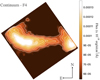 |
Fig. 9 Map of 2.2 μm continuum obtained toward Field4. The background rms is ~0.51 × 10⁻²³ erg s−1 cm−2 Å−1. |
4.1 Field 1
The protostar, understood as the compact object responsible of the jets, lies at the peak of the 2.2 μm continuum emission (see Fig. 6 top panel). The continuum emission morphology is elongated toward the south and it separates into two branches. These features are contained in a region of about 1 arcsec (1400 au at the distance of 1.4 kpc). It is known that continuum emission at 2.2 μm around YSOs can be explained as a scattered light nebulosity, where the light scattering process occurs in the walls of a cavity that was cleared out in the circumstellar material by a jet (e.g., Bik et al. 2006). This is supported by the Brγ and H2 emissions (see Fig. 6 middle and bottom panels), that present some morphological correspondence with both branches of the continuum emission. One of these branches (the southernmost) would seem to be resolved in a probably point-like source with some extended Brγ emission. This possibility is discussed in Sect. 4.4.
The hydrogen Brγ emission line is commonly observed toward massive YSOs (e.g., Cooper et al. 2013). While the majority of Brγ emission detected in the spectra of YSOs is believed to arise from the recombination regions associated with the magnetospheric accretion of circumstellar disk material onto the forming star (Beck et al. 2010; Guo et al. 2021), an additional emission component originating from the strong winds driven by the massive protostar should be important (Davies et al. 2010). The Brγ map that the integral field spectroscopy allows us to construct is useful to study this issue. In our case, the Brγ peak very likely traces the accretion processes, but the extended emission, which has morphological correspondence with the continuum emission, strongly suggests that in this region the Brγ line arises from stellar strong winds (Fedriani et al. 2019) that have probably cleared out the mentioned cavity.
The H2 1–0 S(1) line emission presents an interesting morphology: two cone-like features extending to the north and south, with their respective vertices pointing to the continuum peak (i.e., the position of the protostar). It is important to note that unlike the MHO catalog (Makin & Froebrich 2018) in which it is indicated that this source presents only one H2 lobe whose emission is observed as a collection of knots (the southern emission along the different observed fields in this work), we also detected northward H2 emission. The excitation of this line can be due to collisions or to UV fluorescence. Ratios among different H2 near-IR lines are usually used to distinguish between such excitation mechanisms (see the case of Field 5). However, in Field 1 the 1–0 S(1) is the only H2 line that appears, and thus following Hatch et al. (2005) and Chen et al. (2015) we evaluate the H2 1–0 S(1)/Brγ ratio (see Fig. 13). We obtain ratios ≤1 (with an average of 0.6) along the analyzed region, suggesting a stellar UV excitation mechanism for the H2. This is in agreement with the H2 double cone-shape morphology and the likely cavities carved out in the circumstellar material: the molecular gas lying in the cavity walls is excited by the UV photons from the protostar. Additionally, we note a gradient from the center to the northern and southern borders in such a ratio, reaching to values slightly higher than 1. This can be showing two bipolar thin regions where the H2 excitation may have a collisional contribution.
Finally, it is important to note the absence of CO band-heads at 2.3–2.4 μm, in emission and in absorption. Even though these CO features are usually detected toward YSOs (Hoffmeister et al. 2006; Ilee et al. 2013; Fedriani et al. 2020 and references therein) their nondetection is not rare. As Hoffmeister et al. (2006) mention, the weakness or even the absence of any CO features may therefore be a complex combination of various competing mechanisms. In our case, as in some YSOs studied in Martins et al. (2010), the source presents the combination of H2 1–0 S(1) and Brγ emissions with the absence of CO band-head features. Hoffmeister et al. (2006) found among their large sample of analyzed massive YSOs that the CO featureless objects are basically later than B3, and suggest that they may be similar to other hot YSOs like the Herbig Ae/Be star AB Aurigae (Hartmann et al. 1989). From observations of Herbig Ae/Be stars, Kraus et al. (2008) suggested that the Brγ emission originates in extended stellar or disk winds, which is in agreement with our interpretation of such an emission.
4.2 Fields 2, 3, and 4
Fields 2, 3, and 4 show continuum emission in decreasing intensity (Figs. 7 top, 8, and 9). Except for Field 2, which shows an intense H2 1–0 S(1) bulk of emission (Fig. 7 bottom), these fields do not present emission lines.
In these fields, the continuum emission shows arc-like features that can be resolved into some maximums. In Field 2 the continuum emission presents a zigzagging morphology with three maximums, two of which coincide with the H2 1–0 S(1) emission (see Fig. 7). Given that this is the only H2 line that appears in the region, we cannot study its excitation mechanism. However, based on the observed knots morphology, which is usually found in the shocked gas in HH objects (e.g., Davis et al. 1994; McCoey et al. 2004), we suggest that this emission has a collisional origin due to the passage of a jet which generated a cavity observed in the continuum emission. The continuum zigzagging morphology can be considered as a superposition of two arc-like features, with their concave curvatures pointing to the northwest and east, respectively, whose radii size is about 1200 au in both. Strikingly these features resemble the corkscrew-like structures obtained in computational studies of disk winds, jets, and outflows (Pudritz et al. 2007; Staff et al. 2015). We wonder if we are observing at the near-IR bands the consequences of a jet with complex kinematics. This is discussed below.
In Fields 3 and 4 the near-IR continuum emission also presents an arc-like morphology. In Field 3, an arc with the concave curvature pointing to the north appears in perfect correspondence with the UKIDSS data (see Figs. 8 and 2). Our Gemini data allow us to resolve this arc-like feature into two branches. The radius size of this arc is about 2000 au. In the case of Field 4, while the near-IR continuum emission also has an arc morphology with its concave curvature pointing to the north, it also seems like a filament. These structures reinforces the hypothesis of the presence of a corkscrew-like feature due to the action of a jet.
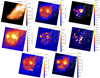 |
Fig. 10 Maps obtained toward Field 5. The 2.2 μm continuum map (top left) is displayed in color scale with contours that are superimposed for comparison in the subsequent continuum subtracted line maps. This figure continues in Fig. 11. The background rms for the corresponding maps are (from top to bottom and left to right) ~2.0, 120, 0.92, 0.78, 100, 0.84, 0.93, and 0.94 × 10⁻²³ erg s−1 cm−2 Å−1. |
4.3 Field 5
Field 5 is characterized by weak continuum emission and the richness of H2 lines (see spectrum in Fig. 5). The maps (see Figs. 10 and 11) show that the line emission does not correlate with the continuum, and they present a circular clump structure. Given that this field could be the end of the jet, we wonder if such a structure is due to shocked molecular gas in a bow shock feature produced by the jet (e.g., O'Connell et al. 2004). The analysis of the line ratios presented in Sect. 3.3 strongly suggests the collisional origin of the H2 emission. As explained in Martín-Hernández et al. (2008), our average values of 11 and 50 obtained in the H2 1–0/2–1 S(1) and 1–0 S(1)/3–2 S(3) ratios, respectively, indicate shocked gas. This is reinforced by the average value of 0.74 obtained in the H2 1–0 Q(1)/1–0 S(1) ratio. Shocked thermal models with a temperature of 2000 K predict a value of 0.7 in this ratio (Luhman et al. 1998; Chen et al. 2015). Thus, given the observed morphology of the molecular emission in this field, it is very likely that we are observing some part of the surface of a bow shock feature projected in the plane of the sky. According to Gustafsson et al. (2010), the morphology of a bow shock projected onto the plane of the sky naturally depends on the viewing angle and on the orientation of the magnetic field. The authors also show that the line brightness and line ratios can change with viewing angle. In Sect. 4.4, we discuss the jet morphology and geometry.
The radial velocity measured for this very likely bow shock is υLSR ~−31 km s−1. Taking into account that the systemic velocity of the source is υLSR = −1.7 km s−1 (Urquhart et al. 2011; and see Sect. 4.5), we conclude that we are observing shocked gas coming toward us. Thus, our Gemini data is tracing a blueshifted jet with a velocity of about 28/cos(i) km s−1, where i is the inclination angle of the jet with respect to the line of sight.
Assuming that we are indeed observing a bow shock in Field 5, or some part of it, by analyzing the moment 1 map presented in Fig. 12, in which the lowest velocities (i.e., more negative) are observed almost at the center of the structure (probably the apex of the bow feature), we conclude that the jet is indeed coming toward us at some inclination along the line of sight. Moreover, the moment 1 map shows a conspicuous velocity gradient with radial velocities increasing from the center toward the border of the structure. Interestingly, toward the north rim a smaller gradient can be seen (green border), which would indicate that the bow shock apex is pointing toward the south. This radial velocity behavior of the bow shock related to MYSO G79 is in agreement with the results exhibited in Fig. 10 of the work of Gustafsson et al. (2010).
It is interesting to note that in most of the H2 maps the circular clump feature presents a clumpy substructure with two maximums, one to the north and the other, which is more intense, almost lying at the center. Structured bow shocks are usually observed in HH objects (Hartigan et al. 2011), and structures that appear as clumps along the bow shock could be due to several phenomena: a thermal instability triggered by strong radiative cooling in the shock, a Kelvin–Helmholtz instability, or even a clumpy preshock density (Suzuki-Vidal et al. 2015; Hansen et al. 2017).
Even though the ratios presented in Sect. 3.3 are quite uniform across the emitting area indicating a uniform mechanism for the H2 emission, they present some variation along the observed structure. In no case do these variations change the interpretation of the H2 excitation mechanism, but they may indicate some different physical conditions in the molecular gas that belongs to the bow shock feature, or they could be a consequence of the bow shock viewing angle (Gustafsson et al. 2010). Precisely by inspecting the results presented by these authors from their 3D model of bow shocks, we find some morphological correspondence with our results. In particular, the modeled morphologies of the H2 1–0 S(1) emission, the 1–0/2–1 S(1) ratio, and the radial velocity distribution of a bow shock observed at an inclination angle along the line of sight i between 20° and 50°, with θ (an angle related to the direction of the assumed uniform magnetic field) between 0° and 30°, are similar to our observational results. Taking into account that Gustafsson et al. (2010) focused on predicting line emission maps of molecular hydrogen in C-type bow shocks, this comparison is in agreement with the fact that we are observing a C-type shock from a YSO jet with a velocity of about 28/cos(i) km s−1 (30–43 km s−1, by considering the i angle range mentioned above), and hence, we are presenting observational evidence that can support the models presented by these authors.
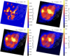 |
Fig. 11 Fig. 10 continued. The background rms for the corresponding maps are (from top to bottom and left to right) ~0.62, 120, 120, and 7.9 × 10⁻²³ erg s−1 cm−2 Å−1. |
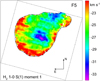 |
Fig. 12 Intensity-weighted mean velocity (moment 1) of the H2 1–0 S(1) line in Field 5. The central velocity of the line is υLSR ~ −31 km s−1. A contour (above 4σ) of the H2 emission is displayed for reference. |
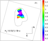 |
Fig. 13 H2 S(1) 1–0/Brγ ratio in Field 1. A contour of the continuum emission (above 4σ) is shown for reference. |
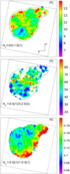 |
Fig. 14 Field 5 ratios: H2 1–0/2–1 S(1), 1–0 S(1)/3–2 S(3), and 1–0 Q(1)/1–0 S(1). A contour (above 4σ) of the H2 1–0 S(1) emission (see Fig. 10) is displayed for reference. |
4.4 Jet morphology, kinematics, and possible causes
In this section we discuss the morphology of the observed near-IR emission and what it can inform us about the kinematics of the jet. Figure 15 displays the UKIDSS Ks emission with contours of the Gemini NIFS data to appreciate a general view of the studied near-IR structure. The continuum at 2.2 μm obtained with NIFS resolves some features observed in the UKIDSS data, and the general view allow us to suggest that the jet is precessing. The observed features at the near-IR continuum resemble the corkscrew-like structures obtained and observed in both computational and observational studies of likely precessing jets (e.g., Rosen & Smith 2004; Movsessian et al. 2007; Paron et al. 2016; Beltrán et al. 2016; Ferrero et al. 2022). For instance, Smith & Rosen (2005) pointed out that the dominant structure produced by a precessing jet is an inward-facing cone, and particularly, a slowly precessing jet leads to helical flows, generating a spiral nebula, as observed in our case. This kind of structure is also obtained in simulations of magnetohydrodynamic disk winds (Pudritz et al. 2007; Staff et al. 2015). The role of magnetic fields can be important in the dynamics of the disk and jets (Pudritz & Ray 2019); however, if one proves a tidal interaction in a binary system, gravity should be the dominant mechanism explaining the jet precession.
We measure the projected wavelength (λp) of the helical pattern (Terquem et al. 1999) by considering the distance between the first curved feature in Field 1 and that of Field 2, obtaining 7000 au. An estimate of the actual wavelength is obtained from λ = λp/sin(i). Considering that the jet velocity can be estimated from υjet = λ/τp, using υjet between 30 and 43 km s−1 (see Sect. 4.3), we obtain a τp of about (1.1–1.8) × 103 yr, which is in agreement with a slow-precessing jet (Smith & Rosen 2005).
The observed angular length of the jet at near-IR, measured from the center of Field 1 to the bow shock observed in Field 5, is about 16 arcsec, which gives a projected length of 0.1 pc at the distance of 1.4 kpc. By considering an inclination angle between 20° and 50° with respect to the line of sight (see Sect. 4.3), we conclude that the length of the jet would be 0.13–0.30 pc, which is an interval of usual values measured in YSO jets (Samal et al. 2018).
By carefully inspecting the 2.2 μm continuum and Brγ emission in Field 1 (see Fig. 16), in which another peak at both emissions appears over one of the branches described in Sect. 4.1, we suggest that MYSO G79 may be composed of a binary system (probably S1 and S2 in the figure). Both sources are separated by 0.″7 (a projected distance of about 980 au at the assumed distance to MYSO G79 of 1.4 kpc). Binarity seems to be something common in MYSOs, and the observed projected binary separation in this case (a lower limit of the actual separation) is within the physical separation range observed in many cases (Pomohaci et al. 2019). Thus, we suggest that the extended near-IR features should be due to a precessing jet that can be explained through the tidal interaction between the companion stars. However, we cannot ignore that the secondary peak of the Brγ emission could be due to a jet knot from the main source, and in this case, if the cause of the jet precession is a binary system, the companion stellar object may be hidden or not resolved in our image.
Radio continuum emission can shed light about the nature of the central stellar object and can give us limits for its spectral type. Sridharan et al. (2002) detected radio continuum emission at 3.6 cm toward MYSO G79 (S3.6 ~1.4 mJy). If it assumed that this emission arises from ionized gas of an optically thin hyperor ultra-compact HII region associated with a young massive star, based on the estimated radio flux density, we can conjecture upon the spectral type of the young star that is generating the observed jet. The number of photons needed to keep a compact HII region ionized, in an optically thin regime, is given by  (Chaisson 1976), where T4 is the electron temperature in units of 104 K, Dkpc is the distance in kiloparsec, vghz is the frequency in GHz, and Sv is the measured total flux density in jansky. We assumed an electron temperature of T = 104 K and a distance of 1.4 kpc. We derived a total amount of ionized photons of about Nuv = 2.6 × 1046 ph s−1. Based on Avedisova (1979) and Martins et al. (2005), the spectral type of the possible young exciting star is later than a B0V. In the case of a binary system, this estimation may correspond to the main source of the system (i.e., the most massive star) or indicates that the ionization generated by both stars is analogous to a star later than B0V.
On the other hand, from more recent observat0ions with high0er angular resolution, Rosero et al. (2019) suggested that the radio continuum emission associated with MYSO G79 arises from an ionized jet. This idea was based on the low radio luminosity (S5 GHzd2 ~ 0.15 μJy kpc2), the spectral index (~0.9), the relatively elongated morphology, and its alignment with the direction of the H2-jet.
For a complete understanding of the spatial configuration of any jet, and hence of the associated extended molecular outflows, it is necessary to be sure which component is coming toward us (blueshifted) and which one is moving away from us (red-shifted), naturally with some inclination along the line of sight. Maud et al. (2015b), who studied outflows in a large sample of sources, based on CO emission showed that MYSO G79 has a redshifted molecular outflow extending toward the southwest (see their Fig. C1). Thus, based on our findings, we decide to reanalyze the CO data, which is presented and discussed in the following section.
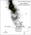 |
Fig. 15 Ks-band emission (in gray) obtained from UKIDSS. The contours in each field are the continuum at 2.2 μm obtained from the NIFS data, except in Field5 where some contours of the H2 S(1) 1–0 emission are displayed. For a better display, the emissions observed with NIFS were slightly smoothed with a boxcar function with a factor of 2. |
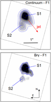 |
Fig. 16 Continuum and Brγ emission toward Field 1 displayed in grayscale with some contours that highlight the presence of two peaks, likely two components of a binary system. These components are called S1 and S2, and the direction of the jet, emerging from S1, is indicated with a red arrow. The separation between S1 and S2 is 0.″7 (a projected distance of about 980 au at the assumed distance of 1.4 kpc). For a better display, both emissions were slightly smoothed with a boxcar function with a factor of 2. The first contours of the continuum and Brγ emissions are 24σ and 4σ, respectively. |
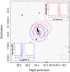 |
Fig. 17 UKIDSS image at Ks band of MYSO G79. The blue and red contours represent the JCMT 12CO J = 3–2 emission averaged from −6 to −12 km s−1 (blue lobe), and from 2 to 8 km s−1 (red lobe), respectively. The blue contours are at 1, 2, and 3 K and the red contours are at 2, 3, and 4 K. The σ noise level is 0.3 K. The averaged spectra (in a beam area) toward the center of the two features are shown. The vertical dashed green lines represent the systemic velocity of the source (at about −1.7 km s−1). The circle of 14.″5 in diameter at the bottom right corner represents the JCMT beam. |
4.5 Molecular gas on a larger spatial scale
In this section we discuss what was obtained by reanalyzing millimeter data from the JCMT and IRAM telescopes with the aim of probing the molecular gas in which MYSO G79 is embedded and likely is affecting.
We reanalyzed the CO data obtained from the JCMT telescope that were presented in Maud et al. (2015b) in order to investigate in detail the molecular outflows related to MYSO G79 (for the description of this data, see Maud et al. 2015b). We found that the spectra of the 12CO data lying toward the northwest of MYSO G79 present a redshifted wing in the velocity range +2 to +8 km s−1, while the 12CO spectra that lie toward the south of G79 has a blueshifted wing in the velocity range −6 to −12 km s−1. Figure 17 displays two spectra showing such spectral wings and the averaged CO emission in these velocity ranges is presented in blue and red contours over the UKIDSS near-IR image. The peak of the blueshifted CO feature coincides with the southern near-IR structure, confirming that the jet is coming toward us along the line of sight. Our finding regarding to the location of the blue- and redshifted molecular gas is the opposite of what was presented in Maud et al. (2015b), and the reason must be that the authors, in the case of this source, included some bulk molecular gas in the determination of the outflows.
Gerner et al. (2014), using data from the IRAM 30 m Telescope, studied the chemistry of 59 high-mass star forming regions, the sample in which MYSO G79 is included. Thus, using these data retrieved from the VizieR Catalog (catalog: J/A+A/563/A97), we analyzed in greater detail the molecular gas, and its chemistry, of the region in which G79 is embedded. The IRAM data consist of an observation of four single spectra at the frequency ranges: 86–90, 90–94, 217–221, and 241–245 GHz centered at RA = 20:23:23.8, Dec = +41:17:40.0 (J2000, almost the center of Field 1). In the case of this source, no molecular line appears in the last frequency range. The beam of the observations at the first two frequency ranges is about 29″, while at the other frequency ranges it is about 11″. Thus, in the first case the spectra probe gas of a region that completely contains MYSO G79 and its jets, while the other spectra probe gas mainly toward the center of the region where the protostar lies (Fields 1 and 2, and the same extension toward the north).
Using the molecular rest frequency database from the National Institute of Standard and Technology (NIST)3, we successfully identified all molecular emission lines that appear in the spectra (see Fig. 18) coinciding with those presented by Gerner et al. (2014) in relation to the source named HMPO20216. In addition to the hyperfine lines of C2H and N2H+, as a novelty, we report the presence of cyanoacetylene (HC3N) at 91.97 GHz, which was not taken into account by Gerner et al. (2014). Given the chemical richness that stands in MYSO G79, we use some molecular lines to obtain information in order to analyze whether the activity of the jets and outflows has influenced the chemistry in the region.
The comparison between the line velocity widths of some molecular species is useful for analyzing the evolutive stage of the region (e.g., Yu & Wang 2015). From this set of data, from Gaussian fittings we measured the FWHM  , and
, and  in 1.36, 1.75, 2.35, 1.33, and 2.11 km s−1, respectively. As was found by Yu & Wang (2015), the velocity widths of HC3N and C2H are similar to that of H13CO+, and the obtained ratios
  and
and  indicate a MYSO in which the effects of the inner jets or the radiation of a possible incipient HII region are not yet evident. As the authors propose, it seems that N2H+ and C2H emissions do not come from the stirred-up gas in the center of the clump.
Additionally, from the isomers HCN and HNC (cyanide and isocyanide hydrogen, respectively) we can estimate the gas kinetic temperature (Tk) over the studied region. From the integrated intensity ratio (I(HCN)/I(HNC)), which in our case is about 2, it is possible to estimate Tk using the expression proposed by Hacar et al. (2020). Such an empirical correlation proposed by the authors yields Tk ~ 20 K for the region in which MYSO G79 is embedded, indicating that these molecular lines are probing cold gas, likely from the envelope in which the source is embedded. If we assume that the I(HCN)/I(HNC) ratio is proportional to the abundance ratio, from the obtained value, and following Hacar et al. (2020) we can say something about the chemical reactions governing these molecular species. We note that slow HNC destruction is occurring at this region with Tk of about 20 K, and hence the predominant mechanism seems to be the neutral-neutral reaction of this molecule with oxygen (HNC + O → NH + CO) rather than involving the H mechanism, which is relevant at Tk > 40 K (HNC + H → HCN + H). The energy barrier of the former reaction has been studied by Hacar et al. (2020) and is proposed to be ∆E ~ 20 K.
We conclude that the complex chemistry revealed by the detection of these molecular species is not a consequence of the jet activity. We point out that these molecular lines probe gas of the external layers of the clump in which MYSO G79 is embedded. This is indeed a very interesting source to be mapped with very high angular resolution at (sub)millimeter wavelengths, for instance, using the Atacama Large Millimeter Array (ALMA).
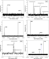 |
Fig. 18 Spectra obtained from the IRAM 30 m Telescope (Gerner et al. 2014) toward the region where MYSO G79 is embedded. The identified molecular species are indicated in each spectrum. For C2H and N2H+ the hyperfine lines are also indicated. |
5 Summary and concluding remarks
Using near-IR integral field spectroscopy, radio continuum, and millimeter data we studied in detail MYSO G79. The analysis of a jet extending southward the source shows corkscrew-like structures at 2.2 μm continuum, strongly suggesting that the jet is precessing. The obtained velocity of this jet is between 30 and 43 km s−1 and it is blueshifted (i.e., the jet is coming toward us along the line of sight). We suggest that the precession may be produced by the gravitational tidal effects generated in a probable binary system, and we estimate a jet precession period of about 103 yr, in agreement with a slow-precessing jet, which can explain the observed helical features. We presented a detailed map of a bow shock produced by such a jet observed coming toward us at an inclination along the line of sight. Given that in the literature there are few works reporting bow shocks from jets driven by MYSOs (e.g., Fedriani et al. 2018), we note that we are presenting an interesting source in which a bow shock generated by a MYSO jet is observed (and resolved) almost from the front. We conclude that we are presenting an interesting observational piece of evidence that can support theoretical models of bow shocks and precessing jets, or that can be used to contrast or to probe such models.
Additionally, we found that the molecular outflow generated by the investigated jet is coming toward us; it is not going away from us, as was stated in a previous work (Maud et al. 2015b). A brief analysis of several molecular species indicates a complex chemistry developing at the external layers of the molecular clump in which G79 is embedded, and it seems that the jet activity does not have any influence on such a chemistry yet. This is a very interesting source to be mapped with ALMA with the aim of resolving the molecular outflows and to study the chemistry of the deepest gas in the clump related to the MYSO activity.
We conclude that in addition to the large MYSO and outflow surveys, dedicated studies of particular sources like this one are extremely useful. This kind of studies, in which data mainly at near-IR and (sub)millimeter wavelengths, are analyzed in depth can shed light on the processes involved in the formation of massive stars and their consequences in the surrounding interstellar medium.
Acknowledgements
We thank the anonymous referee for her/his useful comments and suggestions. Based on observations obtained at the international Gemini Observatory, a program of NSF’s NOIRLab, which is managed by the Association of Universities for Research in Astronomy (AURA) under a cooperative agreement with the National Science Foundation. on behalf of the Gemini Observatory partnership: the National Science Foundation (United States), National Research Council (Canada), Agencia Nacional de Investigación y Desarrollo (Chile), Ministerio de Ciencia, Tecnología e Innovación (Argentina), Ministério da Ciência, Tecnologia, Inovações e Comunicações (Brazil), and Korea Astronomy and Space Science Institute (Republic of Korea). This work was partially supported by grants PICT 2015-1759 and PICT 2017-3301 awarded by Foncyt, and grant PIP 2021 11220200100012 by CONICET. M.B.A. and N.C.M. are doctoral fellows of CONICET, Argentina. S.P., D.M., and M.O. are members of the Carrera del Investigador Científico of CONICET, Argentina.
References
- Areal, M. B., Paron, S., Fariña, C., et al. 2020, A&A, 641, A104 [NASA ADS] [CrossRef] [EDP Sciences] [Google Scholar]
- Avedisova, V. S. 1979, Soviet Ast., 23, 544 [NASA ADS] [Google Scholar]
- Beck, T. L., Bary, J. S., & McGregor, P. J. 2010, ApJ, 722, 1360 [NASA ADS] [CrossRef] [Google Scholar]
- Beltrán, M. T., Cesaroni, R., Moscadelli, L., et al. 2016, A&A, 593, A49 [NASA ADS] [CrossRef] [EDP Sciences] [Google Scholar]
- Beuther, H., Churchwell, E. B., McKee, C. F., & Tan, J. C. 2007, in Protostars and Planets V, eds. B. Reipurth, D. Jewitt, & K. Keil, 165 [Google Scholar]
- Bik, A., Kaper, L., & Waters, L. B. F. M. 2006, A&A, 455, 561 [CrossRef] [EDP Sciences] [Google Scholar]
- Burton, M. G. 1992, Aust. J. Phys., 45, 463 [NASA ADS] [CrossRef] [Google Scholar]
- Caratti o Garatti, A., Stecklum, B., Linz, H., Garcia Lopez, R., & Sanna, A. 2015, A&A, 573, A82 [NASA ADS] [CrossRef] [EDP Sciences] [Google Scholar]
- Chaisson, E. J. 1976, in Frontiers of Astrophysics, ed. E. H. Avrett, 259 [Google Scholar]
- Chen, Z., Nürnberger, D. E. A., Chini, R., Jiang, Z., & Fang, M. 2015, A&A, 578, A82 [NASA ADS] [CrossRef] [EDP Sciences] [Google Scholar]
- Cooper, H. D. B., Lumsden, S. L., Oudmaijer, R. D., et al. 2013, MNRAS, 430, 1125 [NASA ADS] [CrossRef] [Google Scholar]
- Davies, B., Lumsden, S. L., Hoare, M. G., Oudmaijer, R. D., & de Wit, W.-J. 2010, MNRAS, 402, 1504 [Google Scholar]
- Davis, C. J., Eisloeffel, J., & Ray, T. P. 1994, ApJ, 426, L93 [NASA ADS] [CrossRef] [Google Scholar]
- Davis, C. J., Smith, M. D., Stern, L., Kerr, T. H., & Chiar, J. E. 2003, MNRAS, 344, 262 [NASA ADS] [CrossRef] [Google Scholar]
- Davis, C. J., Varricatt, W. P., Todd, S. P., & Ramsay Howat, S. K. 2004, A&A, 425, 981 [NASA ADS] [CrossRef] [EDP Sciences] [Google Scholar]
- Fedriani, R., Caratti o Garatti, A., Coffey, D., et al. 2018, A&A, 616, A126 [NASA ADS] [CrossRef] [EDP Sciences] [Google Scholar]
- Fedriani, R., Caratti o Garatti, A., Purser, S. J. D., et al. 2019, Nat. Commun., 10, 3630 [NASA ADS] [CrossRef] [Google Scholar]
- Fedriani, R., Caratti o Garatti, A., Koutoulaki, M., et al. 2020, A&A, 633, A128 [NASA ADS] [CrossRef] [EDP Sciences] [Google Scholar]
- Ferrero, L. V., Günthardt, G., García, L., et al. 2022, A&A, 657, A110 [NASA ADS] [CrossRef] [EDP Sciences] [Google Scholar]
- Frost, A. J., Oudmaijer, R. D., de Wit, W. J., & Lumsden, S. L. 2019, A&A, 625, A44 [NASA ADS] [CrossRef] [EDP Sciences] [Google Scholar]
- Gerner, T., Beuther, H., Semenov, D., et al. 2014, A&A, 563, A97 [NASA ADS] [CrossRef] [EDP Sciences] [Google Scholar]
- Gredel, R. 2006, A&A, 457, 157 [NASA ADS] [CrossRef] [EDP Sciences] [Google Scholar]
- Guo, Z., Lucas, P. W., Contreras Peña, C., et al. 2021, MNRAS, 504, 830 [NASA ADS] [CrossRef] [Google Scholar]
- Gustafsson, M., Ravkilde, T., Kristensen, L. E., et al. 2010, A&A, 513, A5 [NASA ADS] [CrossRef] [EDP Sciences] [Google Scholar]
- Hacar, A., Bosman, A. D., & van Dishoeck, E. F. 2020, A&A, 635, A4 [NASA ADS] [CrossRef] [EDP Sciences] [Google Scholar]
- Hansen, E. C., Frank, A., Hartigan, P., & Lebedev, S. V. 2017, ApJ, 837, 143 [NASA ADS] [CrossRef] [Google Scholar]
- Hartigan, P., Frank, A., Foster, J. M., et al. 2011, ApJ, 736, 29 [Google Scholar]
- Hartmann, L., Kenyon, S. J., Hewett, R., et al. 1989, ApJ, 338, 1001 [NASA ADS] [CrossRef] [Google Scholar]
- Hatch, N. A., Crawford, C. S., Fabian, A. C., & Johnstone, R. M. 2005, MNRAS, 358, 765 [NASA ADS] [CrossRef] [Google Scholar]
- Hoffmeister, V. H., Chini, R., Scheyda, C. M., et al. 2006, A&A, 457, L29 [NASA ADS] [CrossRef] [EDP Sciences] [Google Scholar]
- Ilee, J. D., Wheelwright, H. E., Oudmaijer, R. D., et al. 2013, MNRAS, 429, 2960 [Google Scholar]
- Kraus, S., Hofmann, K. H., Benisty, M., et al. 2008, A&A, 489, 1157 [NASA ADS] [CrossRef] [EDP Sciences] [Google Scholar]
- Luhman, K. L., Engelbracht, C. W., & Luhman, M. L. 1998, ApJ, 499, 799 [NASA ADS] [CrossRef] [Google Scholar]
- Lumsden, S. L., Hoare, M. G., Urquhart, J. S., et al. 2013, ApJS, 208, 11 [Google Scholar]
- Makin, S. V., & Froebrich, D. 2018, ApJS, 234, 8 [NASA ADS] [CrossRef] [Google Scholar]
- Martín-Hernández, N. L., Bik, A., Puga, E., Nürnberger, D. E. A., & Bronfman, L. 2008, A&A, 489, 229 [NASA ADS] [CrossRef] [EDP Sciences] [Google Scholar]
- Martins, F., Schaerer, D., & Hillier, D. J. 2005, A&A, 436, 1049 [NASA ADS] [CrossRef] [EDP Sciences] [Google Scholar]
- Martins, F., Pomarès, M., Deharveng, L., Zavagno, A., & Bouret, J. C. 2010, A&A, 510, A32 [NASA ADS] [CrossRef] [EDP Sciences] [Google Scholar]
- Maud, L. T., Lumsden, S. L., Moore, T. J. T., et al. 2015a, MNRAS, 452, 637 [Google Scholar]
- Maud, L. T., Moore, T. J. T., Lumsden, S. L., et al. 2015b, MNRAS, 453, 645 [Google Scholar]
- McCoey, C., Giannini, T., Flower, D. R., & Caratti o Garatti, A. 2004, MNRAS, 353, 813 [CrossRef] [Google Scholar]
- McGregor, P. J., Hart, J., Conroy, P. G., et al. 2003, SPIE Conf. Ser., 4841, 1581 [NASA ADS] [Google Scholar]
- McLeod, A. F., Reiter, M., Kuiper, R., Klaassen, P. D., & Evans, C. J. 2018, Nature, 554, 334 [CrossRef] [Google Scholar]
- Movsessian, T. A., Magakian, T. Y., Bally, J., et al. 2007, A&A, 470, 605 [NASA ADS] [CrossRef] [EDP Sciences] [Google Scholar]
- Navarete, F., Damineli, A., Barbosa, C. L., & Blum, R. D. 2015, MNRAS, 450, 4364 [NASA ADS] [CrossRef] [Google Scholar]
- O’Connell, B., Smith, M. D., Davis, C. J., et al. 2004, A&A, 419, 975 [CrossRef] [EDP Sciences] [Google Scholar]
- Paron, S., Fariña, C., & Ortega, M. E. 2016, A&A, 593, A132 [NASA ADS] [CrossRef] [EDP Sciences] [Google Scholar]
- Pomohaci, R., Oudmaijer, R. D., & Goodwin, S. P. 2019, MNRAS, 484, 226 [Google Scholar]
- Pudritz, R. E., & Ray, T. P. 2019, Front. Astron. Space Sci., 6, 54 [Google Scholar]
- Pudritz, R. E., Ouyed, R., Fendt, C., & Brandenburg, A. 2007, in Protostars and Planets V, eds. B. Reipurth, D. Jewitt, & K. Keil, 277 [Google Scholar]
- Rosen, A., & Smith, M. D. 2004, MNRAS, 347, 1097 [NASA ADS] [CrossRef] [Google Scholar]
- Rosero, V., Hofner, P., Kurtz, S., et al. 2019, ApJ, 880, 99 [NASA ADS] [CrossRef] [Google Scholar]
- Ruschel-Dutra, D., Storchi-Bergmann, T., Schnorr-Müller, A., et al. 2021, MNRAS, 507, 74 [NASA ADS] [CrossRef] [Google Scholar]
- Samal, M. R., Chen, W. P., Takami, M., Jose, J., & Froebrich, D. 2018, MNRAS, 477, 4577 [CrossRef] [Google Scholar]
- Sheikhnezami, S., & Fendt, C. 2022, ApJ, 925, 161 [NASA ADS] [CrossRef] [Google Scholar]
- Smith, M. D., & Rosen, A. 2005, MNRAS, 357, 579 [NASA ADS] [CrossRef] [Google Scholar]
- Sridharan, T. K., Beuther, H., Schilke, P., Menten, K. M., & Wyrowski, F. 2002, ApJ, 566, 931 [Google Scholar]
- Staff, J. E., Koning, N., Ouyed, R., Thompson, A., & Pudritz, R. E. 2015, MNRAS, 446, 3975 [Google Scholar]
- Suzuki-Vidal, F., Lebedev, S. V., Ciardi, A., et al. 2015, ApJ, 815, 96 [NASA ADS] [CrossRef] [Google Scholar]
- Tan, J. C., Beltrán, M. T., Caselli, P., et al. 2014, in Protostars and Planets VI, eds. H. Beuther, R. S. Klessen, C. P. Dullemond, & T. Henning, 149 [Google Scholar]
- Terquem, C., Eislöffel, J., Papaloizou, J. C. B., & Nelson, R. P. 1999, ApJ, 512, L131 [Google Scholar]
- Urquhart, J. S., Morgan, L. K., Figura, C. C., et al. 2011, MNRAS, 418, 1689 [NASA ADS] [CrossRef] [Google Scholar]
- Yang, A. Y., Thompson, M. A., Urquhart, J. S., & Tian, W. W. 2018, ApJS, 235, 3 [Google Scholar]
- Yu, N., & Wang, J.-J. 2015, MNRAS, 451, 2507 [NASA ADS] [CrossRef] [Google Scholar]
All Tables
All Figures
|
Fig. 1 Three-color image with the JHKs emission extracted from the UKIRT Infrared Deep Sky Survey (UKIDSS) presented in blue, green, and red, respectively. The bar of 5 arcsec represents a size of ~0.03 pc at the assumed distance of 1.4 kpc. |
| In the text | |
|
Fig. 2 Ks-band emission extracted from the UKIRT Infrared Deep Sky Survey (UKIDSS) toward MYSO G79. The numbered boxes are the 3″ × 3″ fields observed using NIFS at Gemini. The dashed blue circles are the regions from which the spectra presented below were extracted. |
| In the text | |
|
Fig. 3 Spectrum obtained toward a region of about 1.″6 in diameter (see Fig. 2) in which the lines appear in Field 1. |
| In the text | |
|
Fig. 4 Spectrum obtained from a region of about 1.″2 in diameter toward the upper left corner of Field 2 (see Fig. 2). |
| In the text | |
|
Fig. 5 Spectrum obtained from a region of about 2″ in diameter toward almost the center of Field 5 (see Fig. 2). |
| In the text | |
|
Fig. 6 Maps obtained toward Field 1. The 2.2 μm continuum map (top) is displayed in color scale with contours that are superimposed for comparison in the Brγ (middle) and H2 1–0 S(1) (bottom) line emission maps (continuum subtracted). The background rms is ~0.15, 2.97, and 0.65 × 10⁻²³ erg s−1 cm−2Å−1 for the continuum, the Brγ, and the H2 maps respectively. |
| In the text | |
|
Fig. 7 Maps obtained toward Field 2. The 2.2 μm continuum map (top) is displayed in color scale with contours that are superimposed for comparison in the continuum subtracted H2 1–0 S(1) line emission map (bottom). The background rms is ~2.0 and 20 × 10−23 erg s−1 cm−2 Å−1 for the continuum and the H2 maps respectively. |
| In the text | |
|
Fig. 8 Map of the 2.2 μm continuum obtained toward Field 3. The background rms is ~0.56 × 10⁻²³ erg s−1 cm−2 Å−1. |
| In the text | |
|
Fig. 9 Map of 2.2 μm continuum obtained toward Field4. The background rms is ~0.51 × 10⁻²³ erg s−1 cm−2 Å−1. |
| In the text | |
|
Fig. 10 Maps obtained toward Field 5. The 2.2 μm continuum map (top left) is displayed in color scale with contours that are superimposed for comparison in the subsequent continuum subtracted line maps. This figure continues in Fig. 11. The background rms for the corresponding maps are (from top to bottom and left to right) ~2.0, 120, 0.92, 0.78, 100, 0.84, 0.93, and 0.94 × 10⁻²³ erg s−1 cm−2 Å−1. |
| In the text | |
|
Fig. 11 Fig. 10 continued. The background rms for the corresponding maps are (from top to bottom and left to right) ~0.62, 120, 120, and 7.9 × 10⁻²³ erg s−1 cm−2 Å−1. |
| In the text | |
|
Fig. 12 Intensity-weighted mean velocity (moment 1) of the H2 1–0 S(1) line in Field 5. The central velocity of the line is υLSR ~ −31 km s−1. A contour (above 4σ) of the H2 emission is displayed for reference. |
| In the text | |
|
Fig. 13 H2 S(1) 1–0/Brγ ratio in Field 1. A contour of the continuum emission (above 4σ) is shown for reference. |
| In the text | |
|
Fig. 14 Field 5 ratios: H2 1–0/2–1 S(1), 1–0 S(1)/3–2 S(3), and 1–0 Q(1)/1–0 S(1). A contour (above 4σ) of the H2 1–0 S(1) emission (see Fig. 10) is displayed for reference. |
| In the text | |
|
Fig. 15 Ks-band emission (in gray) obtained from UKIDSS. The contours in each field are the continuum at 2.2 μm obtained from the NIFS data, except in Field5 where some contours of the H2 S(1) 1–0 emission are displayed. For a better display, the emissions observed with NIFS were slightly smoothed with a boxcar function with a factor of 2. |
| In the text | |
|
Fig. 16 Continuum and Brγ emission toward Field 1 displayed in grayscale with some contours that highlight the presence of two peaks, likely two components of a binary system. These components are called S1 and S2, and the direction of the jet, emerging from S1, is indicated with a red arrow. The separation between S1 and S2 is 0.″7 (a projected distance of about 980 au at the assumed distance of 1.4 kpc). For a better display, both emissions were slightly smoothed with a boxcar function with a factor of 2. The first contours of the continuum and Brγ emissions are 24σ and 4σ, respectively. |
| In the text | |
|
Fig. 17 UKIDSS image at Ks band of MYSO G79. The blue and red contours represent the JCMT 12CO J = 3–2 emission averaged from −6 to −12 km s−1 (blue lobe), and from 2 to 8 km s−1 (red lobe), respectively. The blue contours are at 1, 2, and 3 K and the red contours are at 2, 3, and 4 K. The σ noise level is 0.3 K. The averaged spectra (in a beam area) toward the center of the two features are shown. The vertical dashed green lines represent the systemic velocity of the source (at about −1.7 km s−1). The circle of 14.″5 in diameter at the bottom right corner represents the JCMT beam. |
| In the text | |
|
Fig. 18 Spectra obtained from the IRAM 30 m Telescope (Gerner et al. 2014) toward the region where MYSO G79 is embedded. The identified molecular species are indicated in each spectrum. For C2H and N2H+ the hyperfine lines are also indicated. |
| In the text | |
Current usage metrics show cumulative count of Article Views (full-text article views including HTML views, PDF and ePub downloads, according to the available data) and Abstracts Views on Vision4Press platform.
Data correspond to usage on the plateform after 2015. The current usage metrics is available 48-96 hours after online publication and is updated daily on week days.
Initial download of the metrics may take a while.