| Issue |
A&A
Volume 667, November 2022
|
|
|---|---|---|
| Article Number | A142 | |
| Number of page(s) | 9 | |
| Section | Planets and planetary systems | |
| DOI | https://doi.org/10.1051/0004-6361/202243576 | |
| Published online | 21 November 2022 | |
Efficiently combining α CenA multi-epoch high-contrast imaging data
Application of K-Stacker to the 80 hours NEAR campaign★
1
Aix Marseille Univ., CNRS, CNES, LAM,
Marseille, France
e-mail: herve.lecoroller@lam.fr
2
Institute of Astronomy, University of Cambridge,
Madingley Road,
Cambridge
CB3 0HA, UK
3
Kavli Institute for Cosmology, University of Cambridge,
Madingley Road,
Cambridge
CB3 0HA, UK
4
Department of Astronomy and Steward Observatory, University of Arizona,
Tucson, AZ, USA
5
European Southern Observatory,
Garching bei München, Germany
6
Université Côte d’Azur, Observatoire de la Côte d’Azur, CNRS, Laboratoire Lagrange,
Nice, France
7
Univ. Grenoble-Alpes, CNRS, IPAG,
38000
Grenoble, France
8
Max-Planck-Institut für Astronomie,
Königstuhl 17,
69117
Heidelberg, Germany
9
Université Paris-Saclay, Université Paris Cité, CEA, CNRS, AIM,
91191
Gif-sur-Yvette, France
Received:
17
March
2022
Accepted:
13
July
2022
Context. Keplerian-Stacker is an algorithm capable of combining multiple observations acquired at different epochs by taking into account the orbital motion of a potential planet present in the images to boost the ultimate detection limit. In 2019, a total of 100 h of observation was allocated to Very Large Telescope (VLT) Spectrometer and Imager for the mid-infrared (VISIR) instrument for the New Earths in the α Centauri Region (NEAR) survey, a collaboration between European Southern Observatory (ESO) and Breakthrough Initiatives, to search for low mass planets in the habitable zone of the α Cen AB binary system. A weak signal (S/N ~ 3) was reported around α Cen A, at a separation of ≃ 1.1 au, corresponding to the habitable zone.
Aims. Our study is aimed at determining whether K-Stacker is also capable of detecting the low-mass planet candidate with similar orbital parameters, which was previously found by the NEAR team. We also aim to search for additional potential candidates around a Cen A by utilizing the orbital motion to boost the signal and by generally placing stronger constraints on the presence of other planets in the system.
Methods. We re-analysed the NEAR data using K-Stacker. This algorithm is a brute-force method that is equipped to find planets in observational time series and to constrain their orbital parameters, even if they have remained undetected in a single epoch.
Results. We scanned a total of about 3.5 × 10⁵ independent orbits, among which close to 15% correspond to fast-moving orbits on which planets cannot be detected without taking into account the orbital motion. We found only a single planet candidate that matches the C1 detection reported in Wagner et al. (2021, Nat. Commun., 12, 922). However, since this constitutes a re-analysis of the same data set, more observations will be necessary to confirm that C1 is indeed a planet and not a disk or other data artifact. Despite the significant amount of time spent on this target, the orbit of this candidate remains poorly constrained due to these observations being closely distributed across 34 days. We argue that future single-target deep surveys would benefit from a K-Stacker based strategy, where the observations would be split over a significant part of the expected orbital period to better constrain the orbital parameters.
Conclusions. This application of K-Stacker to high-contrast imaging data in the mid-infrared demonstrates the capability of this algorithm in aiding the search for Earth-like planets in the habitable zone of the nearest stars with future instruments of the E-ELT, such as METIS.
Key words: methods: observational / methods: data analysis / instrumentation: adaptive optics / stars: individual: Alpha Cen A / instrumentation: high angular resolution / planets and satellites: dynamical evolution and stability
© H. Le Coroller et al. 2022
 Open Access article, published by EDP Sciences, under the terms of the Creative Commons Attribution License (https://creativecommons.org/licenses/by/4.0), which permits unrestricted use, distribution, and reproduction in any medium, provided the original work is properly cited.
This article is published in open access under the Subscribe-to-Open model. Subscribe to A&A to support open access publication.
1 Introduction
High-contrast imaging (HCI) techniques allow planets to be searched for in a relatively large field of view in order to measure their luminosities (intrinsic or reflected), establish their astrometric positions, and determine their orbits. In HCI, observations are aimed at spatially separating the planet from its stellar host, thus allowing for the spectra of detected planets, either using an Integral Field Unit (IFU) or by optically coupling the imager to a high-resolution spectrograph (Otten et al. 2021).
So far, most high contrast imaging instruments (GPI, Macintosh et al. 2014; SCExAO, Jovanovic et al. 2015; SPHERE, Beuzit et al. 2019) have been operating in the near-infrared (≈1–3 µm). This is an optimal choice when looking for young (≤ 100 Myr) giant (a few MJup) planets, for which the typical temperatures range from 1000 to 2000 K, and the contrasts peak in the near-IR. The downside is that these instruments are mostly insensitive to smaller and older planets, which are colder.
Recently, the idea of detecting Earth-like planets in the mid-IR around our closest neighbors (α Cen) has gained attention and some projects aimed at doing so have been closely studied (Kasper et al. 2017; Blain et al. 2018). In the mid-IR, the planet-to-star-contrast ratio is maximized for planets at a few 100 K. In principle, this wavelength range is much better suited to the detection of Earth-like planets. However, the instrumental thermal background is much stronger in the mid-IR than in the near-IR, which complicates the observations. Because of the longer wavelengths, the spatial resolution is also much poorer, with a loss of a factor ≈3–5 in angular resolution between the mid-IR and the near-IR. Still, these downsides of thermal IR observations can be mitigated by focussing on the most nearby stars whose planets would apparently be brighter and observable at greater angular separations.
In addressing these challenges, the New Earths in the Alphα CenRegion (NEAR) experiment has used the deformable secondary mirror at UT4, a new Annular Groove Phase Mask (AGPM) coronagraph optimised for the N-band, and a novel internal chopper system for noise filtering (Kasper et al. 2019) to improve the capabilities of VLT/VISIR in the mid-IR.
In 2019, a survey of 100 h was carried out with VLT/VISIR-NEAR to look for low-mass planets in the habitable zone of the α Cen AB binary system, a 5Gyr old system located at 1.34 pc from our Sun. Using the best 76 h worth of data, Wagner et al. (2021) reported a planet candidate C1 detected at signal-to-noise ratio (S/N) ≈ 3.1–3.5 in the combined data and at S/N ≈ 2.5–2.8 in multiple independent subsets of the data (using only the first eight nights, the last seven nights, or odd or even nights), which makes it unlikely to be a random false positive although a systematic false positive cannot yet be excluded.
In this paper, we re-analyse the NEAR images with the K-Stacker algorithm (Le Coroller et al. 2015, 2020; Nowak et al. 2018), which looks for hidden sources following Keplerian motions in series of high-contrast images. Section 2 presents the data set we used, the K-Stacker algorithm and the main characteristics of the performed search. In Sect. 3, we report on the detection of a possible planet candidate with K-Stacker, which closely corresponds to the C1 candidate also reported in Wagner et al. (2021). We also discuss the gain brought by K-Stacker compared to a simple co-addition of the images. In Sect. 4 we give the completeness map obtained from the non-detection of other sources in our K-Stacker search for companions around α CenA. In Sect. 5, we show that K-Stacker would have been capable of recombining a series of images in which the planet would have moved significantly between observations. We show that this opens up the possibility for using a different observing strategy for such long programs, where the observations would be split over a longer period of time. We argue that this strategy should be followed in the future, notably to schedule the observations only under excellent weather conditions. Finally, our conclusions are given at Sect. 6.
2 Observations and K-Stacker configuration
2.1 Observations
In this work, we use the observations presented in Wagner et al. (2021) of a Cen, acquired using VLT/VISIR-NEAR in N-band filter (central wavelength of 11.25 µm) over a period dating from May 23 to June 27, 2019. Adaptive optics and a vortex coronagraph were used to subtract most of the starlight. The final data products provided by the NEAR team and used by K-Stacker are a set of reduced images at 16 epochs, including a bracketing pair-wise chop subtraction between α CenA and B, systematic artifact removal (detector persistence and filter ghosts), a Karhunen Loeve Image Processing – Angular Differential Imaging (KLIP–ADI) algorithm, and high-pass filtering. The final reduced images were masked along a diagonal strip to hide detector persistence residuals accumulated during the chopping sequence and not fully captured by the artefact model (see Wagner et al. 2021 for further details on the data processing). Following Wagner et al. (2021), we rejected the observation made on May 29, which was of significantly poorer quality. All information about these observations and data reduction can be found in the original paper (see the main article and Supplementary material in Wagner et al. 2021). An example of a fully reduced and masked image is given in Fig. 1.
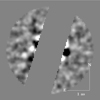 |
Fig. 1 First (2019-05-24) of the 16 VLT/VISIR NEAR observations used to search for a companion to α CenA with K-Stacker. A diagonal strip covering approximately 36% of the field-of-view is masked out to remove defects due to detector persistence. |
2.2 The K-Stacker algorithm
At its core, K-Stacker is an algorithm that looks for the maximum value of the S/NKS as a function of orbital parameters. For each set of orbital parameters tested, the algorithm determines the expected positions x1,…, x16 of the planet at each epoch and integrates the flux at the corresponding position in each image. This gives the signal in each image, namely: s1, …, s16. In parallel, the algorithm also determines the noise levels n1,…, n16 at the same separations (the noise is assumed to be centrosymmetric in each image) by computing the standard deviation of a set values obtained by integrating the flux in 1000 random circles of diameter equal to one Full Width at Half Maximum – Point Spread Function (FWHM-PSF).
The S/N value is then defined as:
 (1)
(1)
Out of all the orbits tested by the algorithm on the grid of orbital parameters, the best 100 orbits are re-optimized using Large-scale Bound-constrained Gradient (L-BFGS-B) optimization algorithm (Zhu et al. 1997). After this step, those orbits which yield a (S/N)KS that is higher than a given threshold (S/N)thresh are considered to be detections of potential planets.
We may note that Eq. (1) does not take into account any correction for small sample statistics, as described in Mawet et al. (2014), and the quadratic sum of the individual noise terms in the denominator is a valid estimate of the total noise only in the case of uncorrelated noise between the different images of the series. Therefore, this (S/N)KS quantity should be regarded only as the “gain function” optimized by our algorithm, and any interpretation in terms of the signal-to-noise ratio should be taken with caution. In particular, we draw attention to the fact that this (S/N)KS cannot be directly compared to the S/N value found by Wagner et al. (2021), which does include a Students’ correction (Mawet et al. 2014), and is based on an estimate of the noise in the centro-symmetric recombined image which takes into account possible correlations between the individual images.
2.3 Search space
As already noted in Wagner et al. (2021), at a separation of ≃1 au, the orbital motion of the planet, corresponding approximately to the size of a resolution element cannot be neglected over the time spanned by the observations. For a circular orbit, the orbital velocity is given by:
 (2)
(2)
where Mstar is the mass of the star expressed in Solar masses, a the semi major-axis expressed in au, and vEarth = 29.8 km s−1 is the Earth’s orbital velocity.
For a face-on circular a = 1 au orbit around α CenA (a 1.1 M⊙ star at 1.34 pc) this corresponds to a projected angular velocity of 12.8 mas day−1, and a total orbital motion of more than 350 mas between the first and last epochs, comparable to the Airy pattern’s full width at half maximum (FWHM). Such displacement can be taken into account by a K-Stacker algorithm (Le Coroller et al. 2020) in order to find the best possible way to combine all epochs accounting for the orbital motion of a putative planet.
We configured K-Stacker to search for planets over the entire field-of-view of the reduced NEAR images (1.5″ in radius), with the persistent diagonal strip masked (see Fig. 1). This corresponds to projected separations ranging from 0.95 to 2 au. We did not constrain the eccentricity and we explored the range 0.00.9. All other parameters are explored over their entire range of possible values, with the notable exception of the stellar parameters (mass and distance), which are taken as fixed values. The number of steps in the grid of parameters explored by the brute-force stage of K-Stacker was determined using an empirical method described in Nowak et al. (2018). A total of 3.5 × 10⁵ orbits with companions positions outside the masks (at the epochs of observation), covering the range of parameters given in Table 1, were set.
3 Recovery of the C1 planet candidate
Over the 3.5 × 10⁵ orbits tested, K-Stacker found 100 orbits that all yield S/N > 5.4 in the recombined image. Following the same method presented in Fig. 2 of Le Coroller et al. (2020), we kept the 84 best orbits corresponding to a relatively constant level of S/N ≈ 5.5, before a first strong decrease. The corresponding combined image is given in Fig. 2.
Although they have different orbital parameters, typically ranging from a = 0.95 au to a = 1.32 au and e spread over the full range of 0 to 0.9 (see corner plots in Fig. 3), all these orbits pass by similar positions at the epochs of observations (see grey curves in Fig. 4). This is evidence of the repeated presence of a significant feature in the data set, whose motion is compatible with Kepler’s laws. Interestingly, the positions at all epochs along these best 84 orbits found by K-Stacker are not only similar between different orbits, but also closely match the astrometric positions derived for the C1 candidate by Wagner et al. (2021). The K-Stacker orbits are slightly to the right of the astrometric points Wagner et al. (2021) at less than a quarter of the instrument PSF of ≈300mas (see grey curves and green crosses in the zoom of Fig. 4). This small systematic discrepancy may be due to the very faint signal (S/N ≈ 1–2) in the Wagner et al. (2021) images to extract the astrometry of CI. Their measurements may have been biased toward the stripes artifact parallel to the chopping direction while K-Stacker is more sensitive to the part of the signal that moves (i.e. less affected by this systematic). Moreover, Wagner et al. (2021) extracted the astrometric positions of C1 via an injection of a negative PSF in groups of two nights (i.e. if the astrometry is shifted at one epoch, it will be also shifted at the next epoch). Finally, most of the K-Stacker orbits have their separations that increase with the epochs, but Fig. 4 shows that a few possible K-Stacker orbits have separations that increase and then decrease, in accordance to the astrometric solutions given by Wagner et al. (2021, see supplementary Fig. 5), where the separation decreases in the last two epochs.
The K-Stacker orbits (Fig. 3) are very similar to the orbital solution derived by Wagner et al. (2021) from their astrometric solutions using a Keplerian model fit (Blunt et al. 2020). Both methods find a semi-major axis a ≈ 1 au with an inclination of i ≈ 60–80 deg, similar to the inclination of the binary’s orbit of 79° (Kervella et al. 2016). The other orbital parameters are not well constrained, due to the limited motion (≈1 PSF) over the range of epochs spanned by the observations (see also discussion in Sect. 5). Overall, the fact that K-Stacker reaches a S/N > 5.4 over 84 different orbits, which all corresponds to positions similar to the one derived by Wagner et al. (2021) for their C1 candidate, leads us to conclude that K-Stacker has detected the same candidate. In accordance with the Wagner et al. (2021) study, the 84 best orbits found by K-Stacker give all a maximum displacement smaller than 6 pixels during the period of observation. Within the error bars, there is no significant gain in terms of S/N obtained using K-Stacker over a simple co-addition of the images, as used in Wagner et al. (2021). Given the limited motion of the candidate over the range of epochs, K-Stacker is also unable to unambiguously distinguish a true planet candidate from, for example, a disk. When masking the candidate in all images and injecting an inclined disk model of similar brightness to C1 (see Supplementary material in Wagner et al. 2021) at a different position angle in the images, K-Stacker also tends to converge towards a solution with S/NKS > 5.0, confusing the edge of a disk with a true planet candidate.
Figure 5 shows the distribution of the maximum displacement along the orbits tested by K-Stacker that peaks at ≈5 pixels (≈half a PSF), but the tail of the distribution reaches a displacement of 11 pixels. Assuming a linear motion of the planet with time, adopting a series of 16 epochs spaced in a similar way as in the observations taken by Wagner et al. (2021) and using the post-ADI PSF structure of the VLT/VISIR observations, we find that the loss in (S/N)KS (without accounting for this motion by computing the noise and signal always at the middle epoch) reaches ≃15% for a total displacement of 7 pixels, and 25% that can not be ignored for a displacement of 11 pixels.
This has two consequences: (1) compared to the co-addition performed by Wagner et al. (2021), our K-Stacker based approach provides a (S/N)KS boost of 15%, for a large number of possible orbits (≃30%), and up to 25% in some cases, which could potentially have led to new detection in the field of view of the NEAR-VISIR reduced images (see Fig. 6, in which we provide an example of the impact of K-Stacker in such a case); (2) the loss in S/N induced by the orbital motion should be accounted for in the calculation of the detection limits.
Search space for K-Stacker run on the NEAR α CenA images.
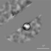 |
Fig. 2 Alpha CenA NEAR images recombined by using the best orbital parameters recovered by K-Stacker (a = 0.96 au, e = 0.78, t0 = −0.11 yr, Ω = 5.34 rad, i = 1.052 rad, θ0 = 0.54 rad). At each epoch, the images are rotated and shifted to put C1 on its periastron position found by K-Stacker, and the frames are co-added. The candidate planet is detected at a (S/N)KS level of 5.5. |
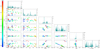 |
Fig. 3 Corner plots of the orbital parameters found by K-Stacker for α CenA CI. At left and bottom: scale of the orbital parameters. Right: scale of the histograms. The 84 points showed in each 2D diagram corresponds to the 84 orbits with the highest (S/N)KS found by K-Stacker. The color of each point gives the K-Stacker signal to noise indicated at left. The origin of the t0 K-Stacker date is 2019 - 05 - 24. |
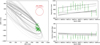 |
Fig. 4 Plot at two dimensions of the orbits projected on the sky, shown on the left. The 84 best orbits found by K-Stacker are shown in grey. The green crosses show the astrometric positions with their error bar given by Wagner et al. (2021). The red circle shows the size of the FWHM-PSF used to integrate the flux in K-Stacker. Right: zoom at the positions found by K-Stacker and Wagner et al. (2021) in ID plots in separation and position angles. |
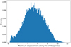 |
Fig. 5 Distribution of the maximum displacement of searched planets along the orbits tested by K-Stacker for the orbital parameters ranges shown at Table 1. |
4 Search completeness analysis
Each term sk in Eq. (1) is the sum of two components: the signal arising from speckles and other sources of noise q, and a potential planet contribution p. Considering an orbit tested by K-Stacker which results in a given value of (S/N)KS and assuming that no planet is present in the images on this orbit, the measured (S/N)KS corresponds only to the speckle and noise contributions. In that case, an additional planet would be detected on this orbit if its integrated fluxes in all images f1,…, f16 is such that:
![$\matrix{{{f_1} + \ldots + {f_{16}}} \hfill \cr {\quad = \left[ {{{\left( {S/N} \right)}_{{\rm{thresh}}}} - {{\left( {S/N} \right)}_{{\rm{KS}}}}} \right] \times \sqrt {{n_1}^2 + {n_2}^2 + \ldots + {n_{16}}^2} .} \hfill \cr }$](/articles/aa/full_html/2022/11/aa43576-22/aa43576-22-eq3.png) (3)
(3)
To relate the f1,…, f16 terms to the true planet to star contrast, the images need to be flux-calibrated. In order to do so, we injected a planet at a contrast ratio of 10-4 in all raw images, and measured the reference planet signal fref1,…, fref16 after the reduction as calculated by K-Stacker at the position where the planet was injected. We performed this injection at several values of separations (ranging from 0.7 to 1.5 au) to take into account the impact of the ADI reduction on the planet flux. The minimum contrast required for the planet to be detected can then be expressed as:
![${C_{\min }} = {{\left[ {{{\left( {S/N} \right)}_{{\rm{thresh}}}} - {{\left( {S/N} \right)}_{{\rm{KS}}}}} \right] \times \sqrt {{n_1}^2 + \ldots + {n_{16}}^2} } \over {{f_{{\rm{ref1}}}} + \ldots + {f_{{\rm{ref16}}}}}} \times {10^{ - 4}}$](/articles/aa/full_html/2022/11/aa43576-22/aa43576-22-eq4.png) (4)
(4)
This equation assumes that all the flux of the planet PSF is properly integrated by K-Stacker. Since we are working with heavily masked images (see Fig. 1), we also need to consider the case when the planet falls behind the masked area. For this, we increase the required minimum contrast Cmin by a factor 1/fout where fout is the fraction of the flux of the PSF actually detectable by K-Stacker (i.e. outside of all masked areas).
We calculated the value of this minimum contrast for each of the 3.5 × 10⁵ orbits tested by K-Stacker, and grouped the results by value of semi-major axis. This gives a set of about 6 × 10⁴ orbits for each of the six values of semi major-axis, covering a range of possible orientation in the images. For each set, we can then proceed to extract the value of the different percentiles of the distribution of Cmin, which give estimates of the probability of detecting a planet at this contrast level with K-Stacker. This method of calculating the detection limits overlooks several different problems, such as the fact that the search on the grid can underestimate the flux of the planet, or the fact that low-flux undetected planets in the images can already contribute to the calculation of the (S/N)KS term of Eq. 4.
To convert the contrast ratios to planetary radii, we used the same method as Wagner et al. (2021). For a given semi major-axis a, the equilibrium temperature of the planet is calculated using:
 (5)
(5)
where Tstar = 5500 K, Rstar = 1.2 R⊙, and AB, the Bond albedo, is 0.3.
The temperature of the planet is set by radiation from the star, plus an extra contribution from internal heating:
 (6)
(6)
To allow for a direct comparison with Wagner et al. (2021), we consider two cases: a hot case with fextra = 0.5 and a cold case with fextra = 0.1. The results obtained for both the cold and hot cases are presented in Fig. 7.
The completeness of our search is typically about 30% at a radius of ≃8 REarth and limited to about 60% for all radii, due to the significant area impacted by defects and excluded of the search area (see Fig. 1).
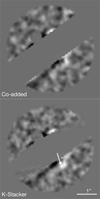 |
Fig. 6 Sum of the 16 reduced images of Wagner et al. (2021), shown at the top, where a fake planet moving of ≈9 pixels along one of the orbit (a = 1.58 au, e = 0.13, t0 = −1.78 yr, Ω = −3.14 rad, i = 0.38 rad, θ0 = 2.2 rad) tested by K-Stacker (see Fig. 5) has been injected at S/N ≈ 1. C1 has been masked by a small circle visible at top-left. The planet is not detectable with a simple co-addition of the images. Bottom: same images recombined by K-Stacker. We detected the planet at the position shown by the arrow at an (S/N)KS ≈ 5. |
5 The case for a more efficient K-Stacker based observing strategy
Wagner et al. (2021) have observed on a short period of one month in order to be able to sum the reduced images at all the epochs without needing to take into account the Keplerian motion to avoid large losses in S/N. This strategy, while it does alleviate the need for an algorithm capable of dealing with Keplerian motion in the recombination (at least in most cases; see Sect. 3 for a discussion on the impact of the orbital motion on the S/N) also significantly hampers our ability to determine the orbital motion of the planet and, thus, its true separation from the star.
Given the ability of K-Stacker to recombine images while properly taking into account the orbital motion, we decided to simulate an hypothetical scenario in which the NEAR observations would have been acquired over a few months, covering a significant part of the expected orbital period (i.e.  for a planet at about one au from α CenA). The NEAR data set was recorded over three weeks in quite variable conditions, so the data should be representative for a campaign of several months as well. The goal was to determine whether or not K-Stacker would have been capable of properly recovering the orbital parameters in such a scenario. To test this scenario, we rotated the NEAR/VISIR reduced images by 180 degrees and injected a fake planet in the reduced images at the same S/N ≈ 1 in each image (i.e. equivalent to injecting a companion at a location of 180 deg from the C1 position), using the best orbital parameters recovered by K-Stacker for the C1 candidate (a = 0.96 au, e = 0.78, t0 = −0.11 yr, Ω = 5.34 rad, and i = 1.052 rad, θ0 = 0.54 rad). Assuming that the observations were obtained regularly (i.e. one image every 11 days) over a period of 6 months (about half of the orbital period), the planet drifts significantly in the images and a naive co-addition results in a non-detection (see Fig. 8). However, when the images are combined with K-Stacker, the planet is detected at a S/N level of 5.5, similar to the S/N obtained on the true C1 candidate (see Fig. 8). The distribution of the most probable orbital parameters resulting from this recombination are given in Fig. 9 and shows that the orbital parameters are overall well constrained, with a strong peak in the distribution around a = 0.95 au, e = 0.7, t0 = −0.18 yr, i = 1.4 rad, Ω = 5.5 rad, and θ0 = 0.1 rad. These results should be compared with the data in Fig. 3, which gives the contraints derived from the observations actually obtained. Although the total observing time is the same in both cases, the orbital parameter estimates are much better when splitting the observations and relying on K-Stacker to perform the recombination properly. In Appendix A, we also provide a second example of the same scenario, using a different set of orbital parameters, with our conclusions remaining unchanged.
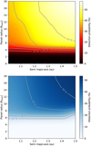 |
Fig. 7 Results of our completeness analysis showing the probability of detecting a planet of a given radius at a given semi major-axis, in the case of a hot planet (upper panel, fextra = 0.5 in Eq. (6)) and a cold planet (bottom panel, fextra = 0.1). |
6 Discussion and conclusion
K-Stacker detected a point source at the same position as the C1 candidate found by Wagner et al. (2021). The (S/N)KS is equal to 5.5 in the recombined image, corresponding to a planet of ≈4 and ≈7 Earth radius, respectively, for the hot and cold models fextra = 0.5 or 0.1 in Eq. (6)). These findings are in very good agreement with the values reported by Wagner et al. (2021).
We show that for ≈15% of the orbits tested by K-Stacker, the inclusion of the orbital motion in the recombination of the images provided a boost of ≃20–25% in terms of S/N. However, despite this boost, we report no new detection in this data set. This study demonstrates, for the first time in mid-infrared high-contrast imaging, that K-Stacker is able to detect hidden planets (here at an S/N ≈ 1 in each image) in a series of images by significantly increasing the S/N values. This new K-Stacker validation is fundamental for future observations. Indeed, Wagner et al. (2021) have been able to detect C1 by summing several observations without taking into account the Keplerian motion smaller than 1 PSF in the mid-infrared during their period of ≈3 weeks of observations. However, this will not be always possible. For example, the detection of C1 in the visible with an instrument like SPHERE-Zimpol would take about 70 h. At visible wavelengths, the orbital motion will be much larger than one PSF over a minimum of ≈30–50 nights required to reach this amount of observing time. Thus, an algorithm such as K-Stacker becomes a key component in establishing such an observation. K-Stacker could also help to search for Jupiter at 3–10 au around the nearest young stars, with the first-generation European Extremely Large Telescope (E-ELT) instruments such as the Multi-AO Imaging Camera for Deep Observations (MICADO) and the High Angular Resolution Monolithic Optical and Near-infrared Integral field spectrograph (HARMONI). Theoretically, an Earth-like planet will be detectable without K-Stacker in 5–10 h with the future Mid-infrared ELT Imager and Spectrograph (METIS) instrument. However, if nothing is detected, K-Stacker will become absolutely necessary to reach the higher contrast with long exposure time under the best atmospheric conditions (i.e. for observations spread over more than 10 days with METIS).
This could be an opportunity to revise our direct-imaging observing strategy, namely: instead of concentrating all the data around a single epoch to allow for a simple stacking of the images, we recommend that the observations be split around several epochs, covering as much of the orbital period as possible, and then recombined using K-Stacker to better constrain the orbital parameters. This K-Stacker strategy will also allow for the scheduling of observations only under excellent weather conditions, in order to reach the ultimate contrast that the instruments can provide. The K-Stacker code is available on gitlab.lam1 and github2. It can be used for both the preparation and exploitation of direct imaging observations with current and future planet imagers.
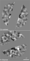 |
Fig. 8 Fake planet has been injected on the same orbit than C1, but with 0.03 yr between each observation (i.e. ≈0.5 yr during the 16 epochs). Top: planet is undetectable when the images are co-added without taking into account the Keplerian motion. Bottom: best recombined image resulting from the K-Stacker run. The planet is easily detected at a (S/N)ks level of ≈5.5. |
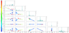 |
Fig. 9 Corner plots of the orbital parameters found on a planet injected on the best C1 K-Stacker orbit but observed during 0.5 yr. At left and bottom: scale of the orbital parameters. At right: scale of the histograms. The 84 points showed in each 2D diagram corresponds to the 84 orbits with the highest (S/N)KS found by K-Stacker. The color of each point gives the K-Stacker (S/N)KS indicated at left. |
Acknowledgments
Acknowledgements. NEAR was made possible by contributions from the Breakthrough Watch program, as well as contributions from the European Southern Observatory, including director’s discretionary time. Breakthrough Watch is managed by the Breakthrough Initiatives, sponsored by the Breakthrough Prize Foundation. K.W. acknowledges support from NASA through the NASA Hubble Fellowship grant HST-HF2-51472.001-A awarded by the Space Telescope Science Institute, which is operated by the Association of Universities for Research in Astronomy, Incorporated, under NASA contract NAS5-26555. This work was supported by the Programme National de Planétologie (PNP) of CNRS-INSU co-funded by CNES. This research has made use of computing facilities operated by CeSAM data center at LAM, Marseille, France.
Appendix A K-Stacker observing strategy gain
In this second example of a hypothetical scenario in which the NEAR images would have been acquired with a different strategy (see Section 5), we have inject a fake planet into the α CenA images (rotated by 180 deg and with CI masked) alongside another possible orbit found by K-Stacker (see Figs. 3 & 4). This orbit corresponds to a larger semi-major axis and a moderate eccentricity (i.e. a = 1.55 au, e = 0.3, t0 = −1.09 yr, Ω = 2.44 rad, i = 1.41 rad, and θ0 = 1.65 rad).
When the observations span a significant part of the orbit (6 months), the histograms of the orbital parameters have their peaks well centered on the injected values (see histograms and star symbol in Fig. A.1). Howerver, when the observations only span a small fraction of the orbit (1 month), the correct orbital parameters are not well recovered (except for t0; see the star symbol that is not at the position of the histogram peaks in Fig. A.2).
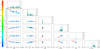 |
Fig. A.1 Corner plots of the orbital parameters found by K-Stacker in a hypothetical scenario in which the NEAR images span a total of 6 months (one observation every 11 days) and assuming that the planet is following an orbit given by a = 1.55 au, e = 0.3, t0 = 0.72 yr, Ω = 2.44 rad, i = 1.41 rad, and θ0 = 1.65 rad. The 84 points showed in each 2D diagram corresponds to the 84 orbits with the highest (S/N)KS found by K-Stacker. The color of each point gives the K-Stacker S/N values indicated at left. The star symbol shows the position of the injected planet in the corner plots. |
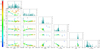 |
Fig. A.2 Corner plots of the orbital parameters found by K-Stacker using the true epochs of observations, as reported in Wagner et al. (2021). The star symbol shows the position of the injected planet in the corner plots (a = 1.55 au, e = 0.3, t0 = 0.72 yr, Ω = 2.44 rad, i = 1.41 rad, and θ0 = 1.65 rad). The 84 points showed in each 2D diagram corresponds to the 84 orbits with the highest (S/N)KS found by K-Stacker. The color of each point gives the K-Stacker S/N values indicated at left. |
References
- Beuzit, J. L., Vigan, A., Mouillet, D., et al. 2019, A&A, 631, A155 [NASA ADS] [CrossRef] [EDP Sciences] [Google Scholar]
- Blain, C., Marois, C., Bradley, C., et al. 2018, SPIE Conf. Ser., 10702, 107024A [NASA ADS] [Google Scholar]
- Blunt, S., Wang, J. J., Angelo, I., et al. 2020, AJ, 159, 89 [NASA ADS] [CrossRef] [Google Scholar]
- Jovanovic, N., Martinache, F., Guyon, O., et al. 2015, PASP, 127, 890 [NASA ADS] [CrossRef] [Google Scholar]
- Kasper, M., Arsenault, R., Käufl, H. U., et al. 2017, The Messenger, 169, 16 [NASA ADS] [Google Scholar]
- Kasper, M., Arsenault, R., Käufl, U., et al. 2019, The Messenger, 178, 5 [Google Scholar]
- Kervella, P., Mignard, F., Mérand, A., & Thévenin, F. 2016, A&A, 594, A107 [NASA ADS] [CrossRef] [EDP Sciences] [Google Scholar]
- Le Coroller, H., Nowak, M., Arnold, L., et al. 2015, in Proceedings of colloquium ’Twenty years of giant exoplanets’ held at Observatoire de Haute Provence, France, October 5-9, 2015, eds. I. Boisse, O. Demangeon, F. Bouchy, & L. Arnold, 59 (Observatoire de Haute-Provence, Institut Pythéas), http://ohp2015.sciencesconf.org [Google Scholar]
- Le Coroller, H., Nowak, M., Delorme, P., et al. 2020, A&A, 639, A113 [NASA ADS] [CrossRef] [EDP Sciences] [Google Scholar]
- Macintosh, B., Graham, J. R., Ingraham, P., et al. 2014, Proc. Natl. Acad. Sci., 111, 12661 [NASA ADS] [CrossRef] [Google Scholar]
- Mawet, D., Milli, J., Wahhaj, Z., et al. 2014, ApJ, 792, 97 [Google Scholar]
- Nowak, M., Le Coroller, H., Arnold, L., et al. 2018, A&A, 615, A144 [NASA ADS] [CrossRef] [EDP Sciences] [Google Scholar]
- Otten, G. P. P. L., Vigan, A., Muslimov, E., et al. 2021, A&A, 646, A150 [EDP Sciences] [Google Scholar]
- Wagner, K., Boehle, A., Pathak, P., et al. 2021, Nat. Commun., 12, 922 [Google Scholar]
- Zhu, C., Byrd, R., Lu, P., & Nocedal, J. 1997, ACM Transac. Math. Softw., 23, 550 [CrossRef] [Google Scholar]
All Tables
All Figures
|
Fig. 1 First (2019-05-24) of the 16 VLT/VISIR NEAR observations used to search for a companion to α CenA with K-Stacker. A diagonal strip covering approximately 36% of the field-of-view is masked out to remove defects due to detector persistence. |
| In the text | |
|
Fig. 2 Alpha CenA NEAR images recombined by using the best orbital parameters recovered by K-Stacker (a = 0.96 au, e = 0.78, t0 = −0.11 yr, Ω = 5.34 rad, i = 1.052 rad, θ0 = 0.54 rad). At each epoch, the images are rotated and shifted to put C1 on its periastron position found by K-Stacker, and the frames are co-added. The candidate planet is detected at a (S/N)KS level of 5.5. |
| In the text | |
|
Fig. 3 Corner plots of the orbital parameters found by K-Stacker for α CenA CI. At left and bottom: scale of the orbital parameters. Right: scale of the histograms. The 84 points showed in each 2D diagram corresponds to the 84 orbits with the highest (S/N)KS found by K-Stacker. The color of each point gives the K-Stacker signal to noise indicated at left. The origin of the t0 K-Stacker date is 2019 - 05 - 24. |
| In the text | |
|
Fig. 4 Plot at two dimensions of the orbits projected on the sky, shown on the left. The 84 best orbits found by K-Stacker are shown in grey. The green crosses show the astrometric positions with their error bar given by Wagner et al. (2021). The red circle shows the size of the FWHM-PSF used to integrate the flux in K-Stacker. Right: zoom at the positions found by K-Stacker and Wagner et al. (2021) in ID plots in separation and position angles. |
| In the text | |
|
Fig. 5 Distribution of the maximum displacement of searched planets along the orbits tested by K-Stacker for the orbital parameters ranges shown at Table 1. |
| In the text | |
|
Fig. 6 Sum of the 16 reduced images of Wagner et al. (2021), shown at the top, where a fake planet moving of ≈9 pixels along one of the orbit (a = 1.58 au, e = 0.13, t0 = −1.78 yr, Ω = −3.14 rad, i = 0.38 rad, θ0 = 2.2 rad) tested by K-Stacker (see Fig. 5) has been injected at S/N ≈ 1. C1 has been masked by a small circle visible at top-left. The planet is not detectable with a simple co-addition of the images. Bottom: same images recombined by K-Stacker. We detected the planet at the position shown by the arrow at an (S/N)KS ≈ 5. |
| In the text | |
|
Fig. 7 Results of our completeness analysis showing the probability of detecting a planet of a given radius at a given semi major-axis, in the case of a hot planet (upper panel, fextra = 0.5 in Eq. (6)) and a cold planet (bottom panel, fextra = 0.1). |
| In the text | |
|
Fig. 8 Fake planet has been injected on the same orbit than C1, but with 0.03 yr between each observation (i.e. ≈0.5 yr during the 16 epochs). Top: planet is undetectable when the images are co-added without taking into account the Keplerian motion. Bottom: best recombined image resulting from the K-Stacker run. The planet is easily detected at a (S/N)ks level of ≈5.5. |
| In the text | |
|
Fig. 9 Corner plots of the orbital parameters found on a planet injected on the best C1 K-Stacker orbit but observed during 0.5 yr. At left and bottom: scale of the orbital parameters. At right: scale of the histograms. The 84 points showed in each 2D diagram corresponds to the 84 orbits with the highest (S/N)KS found by K-Stacker. The color of each point gives the K-Stacker (S/N)KS indicated at left. |
| In the text | |
|
Fig. A.1 Corner plots of the orbital parameters found by K-Stacker in a hypothetical scenario in which the NEAR images span a total of 6 months (one observation every 11 days) and assuming that the planet is following an orbit given by a = 1.55 au, e = 0.3, t0 = 0.72 yr, Ω = 2.44 rad, i = 1.41 rad, and θ0 = 1.65 rad. The 84 points showed in each 2D diagram corresponds to the 84 orbits with the highest (S/N)KS found by K-Stacker. The color of each point gives the K-Stacker S/N values indicated at left. The star symbol shows the position of the injected planet in the corner plots. |
| In the text | |
|
Fig. A.2 Corner plots of the orbital parameters found by K-Stacker using the true epochs of observations, as reported in Wagner et al. (2021). The star symbol shows the position of the injected planet in the corner plots (a = 1.55 au, e = 0.3, t0 = 0.72 yr, Ω = 2.44 rad, i = 1.41 rad, and θ0 = 1.65 rad). The 84 points showed in each 2D diagram corresponds to the 84 orbits with the highest (S/N)KS found by K-Stacker. The color of each point gives the K-Stacker S/N values indicated at left. |
| In the text | |
Current usage metrics show cumulative count of Article Views (full-text article views including HTML views, PDF and ePub downloads, according to the available data) and Abstracts Views on Vision4Press platform.
Data correspond to usage on the plateform after 2015. The current usage metrics is available 48-96 hours after online publication and is updated daily on week days.
Initial download of the metrics may take a while.