| Issue |
A&A
Volume 671, March 2023
|
|
|---|---|---|
| Article Number | A134 | |
| Number of page(s) | 31 | |
| Section | Stellar structure and evolution | |
| DOI | https://doi.org/10.1051/0004-6361/202243519 | |
| Published online | 15 March 2023 | |
Stripped-envelope stars in different metallicity environments
II. Type I supernovae and compact remnants
1
Institute of Astrophysics, FORTH, Dept. of Physics, University of Crete, Voutes, University Campus, 71003
Heraklion, Greece
e-mail: davidrad@ia.forth.gr
2
Argelander-Institut für Astronomie, Universität Bonn, Auf dem Hügel 71, 53121
Bonn, Germany
3
Max-Planck-Institut für Radioastronomie, Auf dem Hügel 69, 53121
Bonn, Germany
4
School of Physics and Astronomy, Monash University, VIC, 3800
Australia
5
Institut d’Astrophysique de Paris, CNRS-Sorbonne Université, 98 bis boulevard Arago, 75014
Paris, France
6
Max-Planck-Institut für Astrophysik, Karl-Schwarzschild-Str. 1, 85748
Garching, Germany
7
Niels Bohr International Academy, Niels Bohr Institute, Blegdamsvej 17, 2100
Copenhagen, Denmark
8
Department of Physics and Astronomy, Seoul National University, Gwanak-gu, Seoul, 08826
Republic of Korea
Received:
10
March
2022
Accepted:
14
December
2022
Stripped-envelope stars can be observed as Wolf-Rayet (WR) stars or as less luminous hydrogen-poor stars with low mass-loss rates and transparent winds. Both types are potential progenitors of Type I core-collapse supernovae (SNe). We used grids of core-collapse models obtained from single helium stars at different metallicities to study the effects of metallicity on the transients and remnants these stars produce. We characterised the surface and core properties of our core-collapse models and investigated their ‘explodability’ using three criteria. In the cases where explosions are predicted, we estimated the ejecta mass, explosion energy, nickel mass, and neutron star (NS) mass. Otherwise, we predicted the mass of the resulting black hole (BH). We constructed a simplified population model and find that the properties of SNe and compact objects depend strongly on metallicity. The ejecta masses and explosion energies for Type Ic SNe are best reproduced by models with Z = 0.04 that exhibit strong winds during core helium burning. This implies that either their mass-loss rates are underestimated or that Type Ic SN progenitors experience mass loss through other mechanisms before exploding. The distributions of ejecta masses, explosion energies, and nickel mass for Type Ib SNe are not well reproduced by progenitor models with WR mass loss, but are better reproduced if we assume no mass loss in progenitors with luminosities below the minimum WR star luminosity. We find that Type Ic SNe become more common as metallicity increases, and that the vast majority of progenitors of Type Ib SNe must be transparent-wind stripped-envelope stars. We find that several models with pre-collapse CO masses of up to ∼30 M⊙ may form ∼3 M⊙ BHs in fallback SNe. This may have important consequences for our understanding of SNe, binary BH and NS systems, X-ray binary systems, and gravitational wave transients.
Key words: stars: massive / supernovae: general / stars: Wolf-Rayet / binaries: general / stars: winds / outflows
© The Authors 2023
 Open Access article, published by EDP Sciences, under the terms of the Creative Commons Attribution License (https://creativecommons.org/licenses/by/4.0), which permits unrestricted use, distribution, and reproduction in any medium, provided the original work is properly cited.
This article is published in open access under the Subscribe to Open model.
Open access funding provided by Max Planck Society.
1. Introduction
Most massive stars are thought to be members of binary or multiple systems that eventually interact via mass transfer (e.g., Sana et al. 2011, 2012, 2014; Moe & Di Stefano 2017). This binary interaction is expected to at least partially remove the hydrogen envelope (e.g., Podsiadlowski et al. 1992; Yoon et al. 2010; Gilkis et al. 2019; Langer et al. 2020; Laplace et al. 2020; Klencki et al. 2020, 2022; Sen et al. 2022), leaving behind a stripped-envelope star. Stripped-envelope stars differ substantially from their hydrogen-rich counterparts in terms of their observational properties, their evolution, and the possible outcomes that they lead to. The most massive and luminous among them are observed to be classical Wolf-Rayet (WR)-type stars. These objects are distinguished by very strong mass-loss rates and optically thick winds, which lead to their characteristic emission-line-dominated spectra, with strong nitrogen (WN sub-class), carbon (WC sub-class), or oxygen features (WO sub-class; see e.g., Crowther 2007 for a review). It has been empirically found that there is a metallicity-dependent threshold luminosity above which stripped-envelope stars may become observable as WR stars. (Shenar et al. 2020). Stars below this luminosity limit are thought to have weaker, optically thin winds (Vink 2017; Sander & Vink 2020). Such stars are also UV-bright, but optically faint, which renders them difficult to observe (Wellstein et al. 2001; Götberg et al. 2017).
In Aguilera-Dena et al. (2022, hereafter referred to as Paper I), we present a grid of detailed 1D evolutionary models of stripped-envelope stars and proposed a method for characterising the minimum WR luminosity as a function of metallicity. We then use stellar evolution models to explore the influence of metallicity during late evolutionary phases of stripped-envelope stars. We find that the properties of our models depend sensitively on the metallicity-dependent mass loss. Combining our theoretical and numerical findings, we constructed a model population of stripped-envelope stars, finding that the populations of WR and transparent-wind stripped-envelope stars are shaped by a combined effect of the minimum WR luminosity and the strength of their mass loss, both of which change as a function of metallicity at different rates.
Stripped-envelope stars are also progenitors of hydrogen-poor supernovae (SNe; of Type IIb, Ib, or Ic), which are characterised by very weak or absent hydrogen features in their spectra near maximum light (e.g., Filippenko 1997). Envelope stripping has been found to have a strong influence on the evolution of massive stars and on the properties that determine what kind of SN explosion they lead to (e.g., Woosley 2019; Schneider et al. 2021; Laplace et al. 2021). With this in mind, in this paper we aim to study the effect of metallicity on stripped-envelope stars through the study of hydrogen-poor SNe, which can be observed in detail at much larger distances than their progenitors. These transients are relatively frequent in the local Universe. The most common are ‘normal’ Type IIb, Type Ib, and Type Ic SNe, which account for around 30% of all nearby core-collapse SNe (Cappellaro et al. 1999; van den Bergh et al. 2005; Prieto et al. 2008; Smartt et al. 2009; Li et al. 2011; Shivvers et al. 2017). Less frequent sub-classes of stripped-envelope SNe include Type Ic-BL SNe, often found in association with long gamma-ray bursts (Hjorth & Bloom 2012), and Type I super-luminous SNe (Perley et al. 2016; Japelj et al. 2016; Schulze et al. 2018), typically found in environments of lower metallicity (Lunnan et al. 2014). A common origin for these transients has been proposed that relies on an evolutionary channel that is different from the ordinary stripped-envelope SNe (Aguilera-Dena et al. 2018, 2020), and their host galaxies have been found to have different properties compared to the typical Type Ic SN hosts (Modjaz et al. 2020).
The absence of hydrogen lines in the spectra of ordinary Type Ib and Type Ic SNe indicates that their progenitors have completely lost their hydrogen-rich envelope by the time they collapse (Dessart et al. 2011; Hachinger et al. 2012). Both SN types have light curves that are often indistinguishable from each other (Drout et al. 2011). However, Type Ib SNe are characterised by helium lines, which are absent in Type Ic SNe. The spectra of Type Ib SNe are consistent with stripped-envelope progenitors that end their evolution with a helium envelope that is rich in nitrogen. On the contrary, Type Ic SNe originate in stripped-envelope stars that have lost this layer through winds and have exposed the products of helium burning (e.g., Dessart et al. 2012, 2020). Modjaz et al. (2011) found that Type Ib and Type IIb SNe typically originate in environments that are less metal rich than Type Ic SNe. These properties indicate that metallicity-dependent wind mass loss is a key factor in the late evolution of their progenitors.
Although massive WR stars are often considered progenitors of hydrogen-poor SNe (Gaskell et al. 1986), the observed ejecta masses (Taddia et al. 2018; Barbarino et al. 2021) are lower than typical WR masses (e.g., Sander et al. 2019). Rather, their observed light curves and spectra are better reproduced by explosion models of relatively low-mass helium stars (e.g., Dessart et al. 2011, 2020). Some SNe have been found to have properties that suggest WR stars as more likely progenitor candidates (e.g., Gal-Yam et al. 2022), but their properties are unusual compared to the majority of the population of stripped-envelope SNe.
Several studies of evolutionary channels for interacting binaries as likely progenitors of Type I core-collapse SNe have also been carried out in recent years. Several approaches have been taken, including detailed binary evolution (e.g., Wellstein & Langer 1999; Yoon et al. 2010, 2017), rapid binary population synthesis (e.g., Zapartas et al. 2017; Kruckow et al. 2018; Vigna-Gómez et al. 2018), and detailed evolutionary calculations of single (e.g., Arnett 1974; Woosley et al. 1995; McClelland & Eldridge 2016; Yoon 2017; Woosley 2019; Ertl et al. 2020) and binary helium stars (e.g., Dewi et al. 2002; Dewi & Pols 2003; Tauris et al. 2015). Evolutionary channels for Type I core-collapse SNe have been widely found in these studies, but explaining the rate, distribution of the ejecta mass, and SN types remains challenging.
In a recent study, Yoon (2017) find that an increase in the metallicity-dependent mass-loss rate observed in carbon-rich WC stars could account for the formation of the faintest WC- and WO-type stars in our Galaxy. The detailed SN light curve and spectral models of Dessart et al. (2020) confirm that an increase in the metallicity-dependent mass-loss rate of WR stars can lead to the production of Type Ic SNe; this results in a sharp dichotomy in the chemical compositions and a change of trend in the initial-to-final mass relation of progenitors of Type Ic and Type Ib SNe.
Unlike the case of Type II SNe, where several progenitors have been directly identified in observations, most attempts to recognise progenitor systems of Type Ibc SNe in archival data of their fields have failed, setting only upper limits (Smartt 2009). As of today, there have only been two progenitor identifications for Type Ib SNe (Cao et al. 2013; Kilpatrick et al. 2021). A candidate progenitor for Type Ic SN was proposed (Kilpatrick et al. 2018), and a candidate for a progenitor companion has recently been reported (Fox et al. 2022). Non-detections place constraints on the progenitor stars of these explosions (and the binary companions, if present), which suggests that they are likely hot and compact (Yoon et al. 2012). The lack of hydrogen in their spectra also sets a stringent constraint on the pre-collapse surface hydrogen abundance of less than 0.001 M⊙ (Dessart et al. 2011). With this in mind, two main evolutionary channels have been proposed to explain the inferred abundances of these SNe: (i) single massive stars that become stripped via strong stellar winds (e.g., Georgy et al. 2009) and (ii) binary stars that have been stripped due to interactions (Podsiadlowski et al. 1992; Langer 2012).
Evidently, variations in surface abundances and metallicity in WR mass loss have a very strong impact on the observed properties of WR stars, as well as the SNe that might result from them. Motivated by this, we study the evolution of helium stars as a proxy for stripped-envelope stars, including wind mass loss, in a fashion similar to Yoon (2017) and Woosley (2019). We extend the initial conditions to cover different metallicity environments, focusing on high metallicities, which are not often addressed in the literature but can account for changes in properties of populations of WR stars and Type I core-collapse SNe. We also pay particular attention to the lower luminosity limit of WR stars through the method found in Paper I and explore its effect on the properties of stripped-envelope SNe.
We have divided the paper as follows: In Sect. 2 we briefly describe the models of stripped-envelope stars at the pre-collapse stage that we use and the methods we employ to analyse them. In Sect. 3 we present our main results, and in Sect. 4 we discuss our predictions for SN and compact-object populations. We finalise our paper with a discussion in Sect. 5 and conclusions in Sect. 6.
2. Method
2.1. Pre-supernova evolution of stripped-envelope stars
To quantify the effect of metallicity on populations of stripped-envelope SNe, we study the structure and composition of grids of stellar evolutionary calculations of helium stars at core collapse, defined as the time when the iron core reaches an infall velocity of more than 1000 km s−1. These core-collapse stellar structure models correspond to the end-points of the evolutionary calculations presented in Paper I. Here, we give a short description of the models, but refer the reader to Paper I for more details on the numerical and physical parameters employed in the stellar evolution calculations. The grids of core-collapse models of non-rotating helium stars models were computed using the Modules for Experiments in Stellar Astrophysics (MESA) code (Paxton et al. 2011, 2013, 2015, 2018), version 10398.
The grids of evolutionary calculations analysed here correspond to seven metallicities, from 0.01 to 0.04 in steps of 0.005, scaled from solar abundances found by Grevesse et al. (1996). Each grid has models with initial masses between 1.5 and 70 M⊙ in steps of 0.5 M⊙. However, only evolutionary sequences with an initial mass greater than 4.0 − 4.5 M⊙ (depending on metallicity) were calculated up to the collapse of the core. Evolutionary sequences with lower initial masses either failed to converge to core collapse because of the presence of off-centre carbon and neon burning layers that are numerically difficult to resolve or did not experience core collapse at all.
The initial models of these calculations were generated through pre-main sequence models of standard composition that were evolved with artificial mixing and no mass loss until core-hydrogen depletion. After that, they were relaxed until thermal equilibrium was reached, without mass loss but with standard mixing. This guarantees that the surface abundances of our models correspond to CNO equilibrium abundances, with enhanced nitrogen and reduced amounts of carbon and oxygen.
Convection was modelled through mixing length theory (Böhm-Vitense 1958), with αMLT = 2.0. We adopted the Ledoux criterion for convection and modelled semi-convection using αSC = 1.0. To calculate the rate of energy generation and changes in chemical composition, we use the approx21 nuclear network in MESA, which includes 21 species from 1H to 56Ni and neutrons.
To avoid convergence issues, we employ MESA’s mlt++ (Paxton et al. 2013), and exclude radiative acceleration in the envelope by setting the velocity to 0 in layers with T > 108 K during the late evolution. We use the mass-loss rates for WN and WC stars of Yoon (2017), who adapts the observed relations of each class, as measured by Hainich et al. (2014) and Tramper et al. (2016), respectively. The mass-loss rates are given by
for Y = 1 − Zinit, and by
for Y < 0.9. The intermediate range is linearly interpolated between the two regimes, using

with x = (1 − Zinit − Y)/(1 − Zinit − 0.9). We set fWR = 1.58, and scale these equations assuming Z⊙ = 0.02.
2.2. Explodability criteria and observable supernova properties
To assess the ‘explodability’ of the core-collapse models, we employ four different tests. First, we measure the so-called compactness parameter at core collapse, as proposed by O’Connor & Ott (2011). It is defined as
and is evaluated at mass coordinate 2.5 M⊙ (and therefore labelled ξ2.5). A high value of this quantity is indicative of a lower probability of a successful SN within the neutrino-driven explosion paradigm. However, a clear boundary between successful and failed SN explosions cannot be drawn from this one-parameter check alone.
To complement this, we employed the two-parameter criterion proposed by Ertl et al. (2016). They propose an explodability test based on a relation between proxies of the core mass and the core density gradient of stars at collapse via the following parameters:
the mass coordinate at the location where the specific entropy, s, is equal to 4; and
The former is thought to be a good proxy of the core mass, while the latter is a measure of the steepness of the density gradient at the same location. Ertl et al. (2016) provide a test using a combination of these two values to determine the final fate of a stellar model.
As a final approach, we use the semi-analytical model proposed by Müller et al. (2016), and the updated version of the same model presented by Mandel & Müller (2020), which includes the effect of fallback onto the newly formed compact object. These semi-analytical models were constructed within the context of the neutrino-driven SN explosion mechanism and were calibrated against the results of 3D numerical simulations. These models also yield predictions for several SN and compact-object observables, such as neutron star (NS) and black hole (BH) gravitational masses, explosion energy, and nickel mass produced in the resulting explosions. Using the predictions for explosion energy and remnant mass, we also calculate the kick velocity imparted on the newly formed compact object following Vigna-Gómez et al. (2018). If the initial energy of the explosion is small, then the asymmetric inner ejecta is expected to fall back completely. This results in a weak explosion launched when the initial ejecta become subsonic. In this case, the transport of energy by the sound pulse becomes decoupled from the transport of matter. The sound pulse quickly becomes spherical, and any explosion asymmetry becomes attenuated. Therefore, in cases where explosion energies are low, the kick velocity is set to 0 km s−1, as it is expected to be very small.
The model of Müller et al. (2016) is a set of equations that treats the pre-explosion and explosion phases of a core-collapse event in a simplified form. The model takes the density, chemical composition, binding energy, sound speed and entropy profiles of a stellar model at core collapse, and computes the amount of mass that is accreted by the proto-NS, and the location of the formed shock as a function of time. It then computes the location of the heating region behind the shock and estimates if and when the neutrino heating conditions become sufficient to trigger an explosion. If the gain region acquires enough energy to produce an explosion, then it calculates the evolution of the NS mass and the explosion energy until they settle to their final state. During the explosion phase, the model accounts for energy input by neutrinos, and energy loss and gain by nuclear disassociation and explosive nuclear burning.
In the version of the model presented by Mandel & Müller (2020), the shock is allowed to propagate further out even if the NS reaches the maximum mass threshold due to ongoing accretion after an explosion has been triggered. The shock is left to evolve until it either exceeds escape velocity (resulting in the termination of accretion onto the remnant) or is attenuated to a weak sound pulse that ejects a small part of the envelope.
These two explosion models depend on several variable parameters that affect the explodability of each stellar model and the properties of successful SN explosions. The main variable parameters in the explosion model are αout, the volume fraction occupied by neutrino-driven outflows far away from the gain radius; αturb, a correction to the expansion of the shock radius due to turbulent stresses; βexpl, the shock compression ratio during the explosion phase; ζ, the efficiency factor for the conversion of accretion energy into neutrino luminosity; τ1.5, the cooling timescale for a 1.5 M⊙ NS and the maximum gravitational mass of a NS.
We calculate the explosion properties of our models with a wide range of values for all parameters. In the main text, we present the outcome of these calculations using a fiducial set of parameters. They correspond to αout = 0.4, αturb = 1.18, βexpl = 4, ζ = 0.75 and τ1.5 = 1.2. We set the maximum NS gravitational mass to 2.05 M⊙. This choice corresponds to a lower value of αout and ζ, compared to the standard values used by Müller et al. (2016). We use this particular combination of parameters, as it more closely resembles the outcome expected from the use of the Ertl et al. (2016) explodability criterion. We discuss the impact of parameter variation, as well as the impact of the binding energy that is used to calculate the outcome of the explosions in the Appendix B. Models from Set B, presented in Appendix B.2, correspond to those used by Antoniadis et al. (2022).
2.3. Population synthesis models
To gain a better understanding of how the measurable parameters of Type I SN explosions evolve as a function of metallicity, we generated populations of helium stars in a similar way as described in Paper I. We randomly sample main sequence stars from a Salpeter initial mass function (IMF; Salpeter 1955), and use the relation between zero-age main sequence (ZAMS) and helium core masses from Woosley (2019), given by
We count the number of transients generated, independently of the lifetime of helium stars, assuming a constant star-formation rate, and convolve this with our results from Sect. 3.2. Counting every transient generated from this sampling, assuming that they are all stripped, and then looking at the relative distribution of their properties is equivalent to assuming that the stripping probability is the same at each mass, and ignores the contribution of Type Ib and Type Ic SNe that are generated through other channels. While the assumptions in this population model are an oversimplification, they allow us to crudely estimate how the fate of stripped-envelope stars change across cosmic time.
A caveat in our calculations is that our models with initial masses below 4 − 4.5 M⊙ do not reach core collapse, since they ignite nuclear burning above a degenerate core and experience convergence problems. Therefore, we cannot assess the minimum mass at which stars produce SNe, and stars with masses smaller than our least massive core-collapse model that produce SNe cannot be analysed using the Müller et al. (2016) model; which does not allow us to infer their explosion properties. To account for the number of successful SNe regardless of the results of our evolutionary calculations, we follow Chanlaridis et al. (2022) and set the lower limit in the initial helium core mass for core collapse at 3 M⊙, which they find to be metallicity independent if no core overshooting is included during helium burning. This is further justified since stripped-envelope stars of this mass are always below  , implying that their mass-loss rates are very small during core helium burning (although they may experience intense mass loss after core helium depletion; see Chanlaridis et al. 2022). Consequently, the evolution of stripped-envelope stars near the boundary between core-collapse progenitors and white dwarfs or thermonuclear explosions is similar, independent of their initial chemical composition. We estimate the distribution of observables in this regime by extrapolating our finding for higher-mass stars. More specifically, NS gravitational masses are assigned a random value between 1.22 and 1.3 M⊙, explosion energies are in the range of 0.5–0.8×1051 erg, and nickel masses are in the range 0.04–0.15 M⊙. Kick velocities are assigned through these values, according to Eq. (2) of Mandel & Müller (2020), and the mass of the ejecta is inferred by extrapolating the initial mass–final mass relation and removing the corresponding baryonic mass that was lost to the formation of the NS (see below for further justification).
3. Impact of metallicity on Type I supernovae and compact remnants
In this section we study the effect of metallicity on the structure and chemical composition of stripped-envelope stars at the end of their evolution, and how it affects the transients that they produce. To do this, we characterise the final output of the models described Paper I. To remain consistent in our notation, in Table 1 we recall the definitions of key quantities from Paper I, which are important for the analysis of the core-collapse models.
Notation definitions.
To determine the stellar models for which our wind prescriptions are accurate, we employ the analytical method derived in Paper I to find the metallicity-dependent transition luminosity between WR stars and their low-mass counterparts, which have optically thin winds and lower mass-loss rates. That is, we set these luminosities as follows:
For WC-type stars, the fit to the observations takes the form of
These luminosities are converted to stellar mass estimates using the mass-luminosity relation of Langer (1989). The explosion properties of stripped-envelope stars with luminosities below the minimum WR luminosities are also shown, but the implications of lower mass-loss rates on transparent-wind stripped-envelope stars are considered a posteriori.
We have subdivided this section into the following parts: in Sect. 3.1 we present the distribution of final masses and surface chemical compositions in our models. In Sect. 3.2 we characterise the internal structure of our models at core collapse and apply several tests to assess which models are more likely to produce SNe and which ones are more likely to form BHs as a result of core collapse.
3.1. Pre-collapse masses and chemical compositions of Type I supernova progenitors
The pre-collapse masses of our helium-star models, presented in Fig. 1, are determined by an interplay between their lifetime and the intensity of their winds. A change in the trend in their final mass occurs between around 7 and 11 M⊙, indicated by dots in Fig. 1, and is also observed in the models of Yoon (2017) and Woosley (2019). As discussed in Paper I, it corresponds to the metallicity-dependent transition mass between stars that lose mass as WNs for most of their lives and those that spend a significant time as WC and WO stars with stronger mass-loss rates. The ejecta mass of SNe can be estimated, to first order, from Fig. 1, but a thorough analysis of this is presented in Sects. 3.2 and 4.
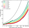 |
Fig. 1. Final mass (at core collapse) as a function of initial mass for helium star models of different metallicities. The dots on each line indicate, for each metallicity, the initial helium star mass at which the transition between WN- and WC-type mass loss is observed to occur in the models. The rhombi indicate the value of the minimum luminosity WN-type models obtained from Eq. (8), and using the mass-luminosity relation of Langer (1989). Helium stars below this limit do not have optically thick WR winds and have overestimated mass-loss rates. |
The type of SN that helium stars may produce depends not only on the final mass or ejecta mass, but also on the mass and composition of their envelope (Dessart et al. 2020). According to Hachinger et al. (2012), approximately only 0.01 M⊙ of helium in the envelope of a hydrogen-poor star at core collapse is enough to produce detectable helium lines in the SN spectrum. This would render all of our Type Ib SNe progenitor models candidates. However, Dessart et al. (2011, 2012) determined that the spectral type is sensitive not only to the helium mass but also to the envelope composition at core collapse and the mixing that takes place during the SN explosion. Furthermore, the model spectra of Dessart et al. (2020), produced by progenitors similar to ours, show that Type Ic SNe spectra can be produced by helium stars if their mass loss is strong enough to remove the helium-nitrogen envelope. Thus, there is a sharp transition between the evolution of progenitors of Type Ib and Ic SNe, which roughly corresponds to the transition between WN- and WC-type stars. A peculiar large-scale mixing of nickel and helium might cause some WN-type progenitors to appear as Type Ic SNe. Although helium-deficient WR stars can only produce Type Ic SNe, the complexity of 3D mixing and the excitation of HeI lines by non-thermal processes do not exclude the possibility that some helium-rich WR progenitors appear as helium-deficient Type Ic SNe.
Figure 2 shows the remaining mass of helium in the envelope as a function of the initial mass at the time of core collapse. We calculated this quantity as
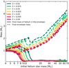 |
Fig. 2. Final mass of helium in the envelope, as calculated by Eq. (10), shown in solid lines as a function of the initial mass of helium stars of different metallicities. The final total mass of the helium-rich envelope is shown in dashed lines for comparison. The dots on each line indicate, for each metallicity, the initial helium star mass at which the transition between WN- and WC-type mass loss is observed to occur in the models. The rhombi indicate the value of the minimum initial mass above which helium stars are observable as WN-type stars, obtained via Eq. (8). Helium stars below this limit do not have optically thick WR winds and have overestimated mass-loss rates. |
where, by only considering the regions with temperature smaller than 108 K, we exclude the helium formed in the core during collapse, thereby accounting for only the envelope content. We note that this is different from the envelope mass (i.e. the total mass above the carbon-oxygen core), since only the mass in the form of helium is accounted for.
As shown in Fig. 2, our helium star models sharply transition from having abundant helium in their envelope to having only very little. Most models that lose mass as WN stars throughout their evolution have between 0.8 and 1.4 M⊙ of helium in their envelopes. On the other hand, the amount of helium in the envelope converges at a value of around 0.2 M⊙ for models with initial masses large enough to produce WC-type stars (denoted by dots in the figure), with very few models reaching core collapse between these two regimes. However, as shown in Fig. 2, the total final envelope mass increases monotonically with the initial helium star mass, except at the point where stars transition into the WC regime.
The position where this transition occurs depends on metallicity, but models with intermediate helium masses occur at all metallicities and may lead to SNe with ‘intermediate’ spectra between a Type Ib and a Type Ic (see model he9 from Dessart et al. 2020). Since the number of models that were found in this transition region is small, and it is impossible to determine the exact width of the parameter space in the intermediate region without performing detailed radiation transfer models, we chose the presence or absence of a nitrogen- and helium-rich envelope to distinguish models we classify as possible progenitors of Type Ib SNe, from those that we classify as possible progenitors of Type Ic SNe. We highlight, however, that the exact spectral properties of a Type I SN depend on nickel mixing, and some WN-type stars may also produce Type Ic SNe.
Contrary to the convective helium-burning cores of hydrogen-rich stars, the convective cores of helium stars shrink in size as they evolve. As their convective cores decrease in mass, a smooth composition gradient develops in the formerly convective region, followed by a sharp transition between the helium and nitrogen envelopes and the layers enriched with carbon and oxygen. The layers directly above the helium-free core later become part of a convective helium-burning shell, which can grow in mass due to the smooth composition gradient left behind by the gradual retreat of the convective helium core. This means that most of the helium is stored in the nitrogen-rich envelope, and stars that lose these layers have a similarly low amount of helium at core collapse.
However, the total helium mass is not the only factor that determines whether a star explodes as a Type Ib or a Type Ic SN. Figure 3 shows the behaviour of the surface abundances of He, C, N, and O in our core-collapse models as a function of the initial mass. As can be seen, there is a clear dichotomy in the surface chemical composition. In particular, we find a steep change in N abundance and also a gradual reduction of He and an increase of C and O as a function of initial mass, transitioning from CNO equilibrium abundances to the abundances that result from helium burning. Our models have a sharp divide between these two populations of helium stars with no intermediate cases. The surface nitrogen abundance has the sharpest drop since it burns at a temperature lower than that of helium, leading to a sharp transition in its abundance between the initially convective region and the envelope. The absence of nitrogen-rich layers corresponds to the transition between Type Ib and intermediate Type Ibc and Type Ic spectra in Dessart et al. (2020). Therefore, we use that as the dividing line between the two cases in the following sections.
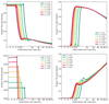 |
Fig. 3. Surface mass fractions of 4He, 12C, 14N, and 16O of our helium star models at core collapse, as a function of initial mass, for different metallicities. The dots on each line indicate, for each metallicity, the initial helium star mass at which the transition between WN- and WC-type mass loss is observed to occur in the models. |
As the initial mass increases, there is a trend for the carbon abundance to initially increase and then decrease again. A similar trend is observed for surface oxygen, except that the trend has a local maximum and a minimum before continuing to increase for the highest final masses. Above ∼20 M⊙, final surface abundances seem to depend primarily on the initial mass. This implies that this quantity is determined early in the evolution and leads to small variations in the surface abundances for models of similar final mass, independent of metallicity.
The two observed trends of change of final composition as a function of initial mass correspond to the change in mass-loss rate. The decrease in helium and nitrogen between 7 and 12 M⊙ (depending on metallicity) occurs when a model initially exposes the layers that were formerly part of the convective helium core. This change is accompanied by an increase in the mass-loss rate. The increased mass-loss rate also causes the convective core to retreat at a faster rate (see Fig. 1 in Paper I). The second trend, beginning around 10–18 M⊙, corresponds to models that expose layers that were part of the convective core after the mass loss increased, which caused the chemical gradient to be different as a result of the increase in the mass-loss rate.
3.2. Properties of supernova explosions from stripped-envelope stars
Since the final masses and surface compositions of models of stripped-envelope stars with similar initial masses change with metallicity, the relative rate of different SN types coming from them is also metallicity dependent. This is a consequence of the way that the type of SN depends on the chemical composition of the surface (Dessart et al. 2020). However, SN rates also depend on the number of stars that actually become SNe, instead of collapsing into a BH directly (Patton & Sukhbold 2020). The change in the chemical composition of the surface with mass and metallicity has been addressed in Sect. 3.1. The latter issue is discussed here. First, we discuss the carbon-oxygen core masses and central carbon content at the end of helium burning in our models. Then, to gauge the explodability of our core-collapse models, we employ the four methods described in Sect. 2. The results from these analyses are discussed here, and a different visualisation of the outcome of these tests is presented in the Appendix.
The carbon core mass and the carbon mass fraction at the end of helium burning are quantities that will influence the subsequent carbon and neon burning stages and the final fates of helium stars of different helium masses and metallicities (Chieffi & Limongi 2020; Patton & Sukhbold 2020; Sukhbold & Adams 2020). Lower core carbon abundances at the end of helium burning result in weaker carbon burning, which does not require convection to transport the energy generated away from the burning region. This will impact the structure of the core, making it more compact, resulting in a higher gravitational binding energy, and therefore SN explosions are less likely to occur as the metallicity increases (Sukhbold & Woosley 2014). We find that our helium star models of the same initial mass will progressively have less massive carbon-oxygen cores as metallicity increases, as shown in the top panel of Fig. 4. More massive carbon-oxygen core masses will in turn result in a lower central carbon mass fraction at the end of helium burning, as shown in the bottom panel.
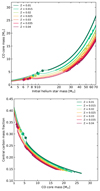 |
Fig. 4. Properties of the carbon-oxygen core at the end of helium burning. Top: carbon-oxygen core mass at the end of helium burning, as a function of initial helium star mass. Bottom: central carbon abundance at the end of helium burning, as a function of carbon-oxygen core mass. Thin lines represent models where core carbon burning occurs convectively, whereas thick lines represent models where carbon burning occurs radiatively. The dots on each line indicate, for each metallicity, the initial helium star mass at which the transition between WN- and WC-type mass loss is observed to occur in the models. The rhombi indicate the value of the minimum initial mass above which helium stars are observable as WN-type stars, obtained via Eq. (8). Helium stars below this limit do not have optically thick WR winds and have overestimated mass-loss rates. |
The threshold mass above which models spend some time as WC-type stars before core collapse corresponds to the change in the trend of final mass as a function of initial helium mass (see Fig. 1), and this division is accompanied by different trends in carbon-oxygen core masses and central carbon mass fractions at the end of helium burning as a function of initial mass. This is broadly consistent with the results of Schneider et al. (2021) but shows that the dependence of WR winds on metallicity and surface composition (or WR type) has a strong impact on the core evolution of helium stars.
Figure 5 shows the compactness parameter at core collapse of our models, as a function of both the initial helium star mass and the final mass. Because helium stars experience shrinking of their convective core during helium burning, a helium star of a given initial mass will often have a lower compactness than a hydrogen-rich, non-stripped star whose ZAMS mass corresponds to the same helium core mass at the beginning of core helium burning, and the first sharp increase in the value of ξ2.5 will occur at a corresponding lower ZAMS mass than for stars with a hydrogen envelope (Schneider et al. 2021; Laplace et al. 2021).
 |
Fig. 5. Compactness parameter as a function of initial mass (top) and final mass (bottom) for helium star models of different metallicities. Circles represent models with final surface abundances that correspond to Type Ib SN progenitors, whereas crosses represent models with surface abundances that correspond to Type Ic SN progenitors. The dashed horizontal line at ξ2.5 = 0.35 divides the majority of exploding models from those that produce BHs. |
We observe a general trend for features in the behaviour of compactness as a function of initial helium star mass, such as peaks and valleys, to be displaced to higher initial helium star masses with increasing metallicity, correlated with the drop in final mass for similar initial masses, as shown in the bottom panel of Fig. 5.
Although the compactness parameter alone is not enough to determine whether a stellar model at core collapse will lead to a successful neutrino-driven SN explosion or not, we find that most cases with ξ2.5 < 0.35 are predicted to explode according to the Ertl et al. (2016) test, as well as with the Müller et al. (2016) test (see Fig. A.1). At every metallicity, we find that most helium star models with initial mass below ∼35–40 M⊙ will produce successful explosions, with a few exceptions located mostly at the peak in ξ2.5, found at a final mass of around 8 M⊙. The similarity in ξ2.5 for models with similar final masses is due to the fact that the final mass is roughly determined before the beginning of carbon burning. The remaining lifetime is too short for stars to lose a significant amount of mass, and since the core structure is mostly determined by the mass of the carbon oxygen core, features such as the transition between models with convective and radiative core carbon burning occur at similar final masses, correlated to the first peak in ξ2.5 (Sukhbold & Woosley 2014). However, variations occur between models with similar masses at different metallicities, likely related to differences in their core composition and mass, and although subtle, they have an effect on the outcome of SN and compact object populations that result from our models (see Sect. 4).
An interesting feature in the behaviour of ξ2.5 appears at final masses greater than 15 M⊙, where we find a region in which two solutions to the compactness parameter appear. The two branches of the values of the compactness parameter models in this region correspond to values of ξ2.5 between 0.4–0.6 and 0.6–0.8. All values are above the limit of ξ2.5 ∼ 0.35 where we expect to find exploding models, and all models are predicted to form BHs without SNe, according to both the Ertl et al. (2016) and the Müller et al. (2016) tests with our choice of parameters. However, variations in the parameter values in the Müller et al. (2016) model can lead to SN explosions in this regime, and some of these progenitor models are expected to produce fallback SNe and BHs in the lower-mass gap, when analysed with the Mandel & Müller (2020) model (see Fig. A.2). Because all of the explosions predicted in this regime are powered by fallback, we refer to this region as the ‘island of fallback explodability’ (see Antoniadis et al. 2022, for a discussion). The exact number of fallback SNe, as well as their properties, depend sensitively on the model parameters. However, every set of parameters we explored produces at least some fallback SNe in this regime (see Appendix B). Explosions could also be facilitated in this regime by the presence of strong rotation (e.g., Aguilera-Dena et al. 2020), which can produce successful SN explosions even when neutrino emission is not enough to revive the SN shock (e.g., Summa et al. 2018). However, rotation is not expected to be high in the cores of stripped-envelope stars formed by case A and case B mass transfer due to the loss of angular momentum during this phase (Yoon et al. 2010).
For the fiducial set of parameters that we employed (see Sect 2.2), the explodability, and the estimates for the explosion energies, gravitational masses of NSs and BHs, and nickel masses obtained by analysing our models with the Müller et al. (2016) and Mandel & Müller (2020) are summarised in Figs. 6 and 7, respectively. The black line in the figures indicates the value of the minimum mass above which models evolve as WC-type stars, which we take as a threshold below which successfully exploding stars are expected to be observable as Type Ib SNe and above as Type Ic. We find that most of these quantities are comparable to those inferred from stripped-envelope SN observations (e.g., Taddia et al. 2018; Barbarino et al. 2021), but discuss this in more detail in Sect. 4.
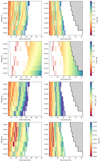 |
Fig. 6. Summary of key parameters obtained from the core-collapse models of helium stars through the explosion model of Müller et al. (2016), as a function of the initial mass (left) and the final mass (right). We include the NS gravitational mass obtained for core-collapse models that successfully explode, the BH mass for models that directly collapse (which corresponds to their final mass), the explosion energy, and the nickel mass. The dashed black lines indicate the division between Type Ib and Type Ic progenitors, and the hashed region corresponds to areas that our model grid does not cover. The horizontal dashed line corresponds to the minimum mass above which models reach core collapse as a WC- or WO-type star, and models to the right of this line are therefore expected to be Type Ic SN progenitors. |
As Ertl et al. (2020) had already found with their models with enhanced mass loss, the initial (helium) masses of stars located in the so-called islands of explodability become displaced if wind mass-loss rates are different. However, as Figs. 6 and 7 suggest, the final mass is not the only defining factor that determines the explodability of a model and the properties it will have upon explosion. A region around final masses of ∼8 M⊙ exists where low-mass BHs can form for most metallicities, but the location and extent of this region varies significantly as a function of metallicity. There is a tendency for the highest final mass where explosions occur to increase with decreasing metallicity (see Fig. 6 and Sect. 4). This implies that explosions with high ejecta masses are more likely to occur in environments with low metallicity. Such explosions also tend to be more energetic. However, the exact morphology and location of these regions depend on the choice of parameters in the Müller et al. (2016) model. Because the maximum ejecta mass of Type Ic SNe decreases in high-metallicity environments, the minimum mass of BHs that come from these very massive stars decreases twofold, both because of the increase in mass loss and also because of this effect.
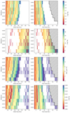 |
Fig. 7. Same as Fig. 6, but using the explosion model of Mandel & Müller (2020), which includes the effect of fallback. |
As shown in Fig. 7, the number and mass of models that experience fallback also vary as a function of metallicity, but it is a relatively small number. Many fallback SNe are predicted to be more energetic explosions (with energies ranging from 6 × 1051) erg, and up to a few times 1052 erg), with nickel masses higher than those of the rest of the sample (often in excess of 0.2 M⊙). Including the effect of fallback in our model does not change the predictions of the properties of the explosions we calculated without including fallback but produces models that successfully explode in places where explosions were not originally expected. However, this depends on the input parameters of the model, and we may underestimate transients that originate from progenitors of lower mass, which are likely more numerous in the Universe (see Appendix B).
The NS gravitational masses predicted for our models range between 1.32 and 2.03 M⊙. It is noteworthy that we observe a tight correlation between compactness and NS mass (see Fig. A.3), and that the smallest NS mass is larger than the least massive known NS (Antoniadis et al. 2016). We attribute this to the lack of core-collapse models below 4 M⊙ in our grid. The maximum NS mass we find is close to the maximum known NS mass (Cromartie et al. 2020), and it is also close to the limit of 2.05 M⊙ that is imposed in the Müller et al. (2016) model. Exploring the effect of variations on this maximum mass in the resulting SN parameters might help us understand the origin of the distribution of the NS mass distribution, but is beyond the scope of this work.
The real distribution of compact object masses cannot be directly drawn from our single stellar models. One reason for this, in particular for BH masses, is that the range of final masses in our models, which will roughly correspond to the range in BH masses, is metallicity dependent. Another reason is that we do not have models in the range of (pulsational) pair instability, which will in turn determine the maximum mass of BHs. Furthermore, binarity might have a role in determining the distribution of BH masses in the Universe beyond that of creating stripped-envelope stars. However, this distribution has been computed by other authors in different works (Farmer et al. 2020; Woosley & Heger 2021), and is particularly relevant at metallicities lower than those of our models. Low-metallicity environments are believed to be more efficient in producing the binary BHs that we observe today as mergers (e.g., Neijssel et al. 2019).
However, we can draw some conclusions from the distributions in Figs. 6 and 7. For instance, a lower-mass BH population comes for models with final masses of around 6–9 M⊙. This distribution will dominate the BH mass distribution, as is favoured by the IMF, and the number and mass of the said BHs will depend on the metallicity. The BHs in this regime produced at low metallicity will peak at the final masses of low metallicity models, since they correspond to stars of lower initial mass. Similarly, the most massive BHs formed by helium stars will be formed at low metallicity, regardless of whether the maximum BH mass depends on or not in metallicity. In the case where the effect of fallback is considered, we also expect a population of mass-gap BHs to appear.
The explosion energies predicted for our models range from approximately 0.5 × 1051 erg, up to approximately 5.6 × 1051 erg; and the kinetic energy is correlated with the final mass (see Fig. A.3), likely due to its dependence on the binding energy of the progenitor at core collapse. We find that the most energetic explosions correspond to those models that have higher values of ξ2.5, which also correlates with high values of μ4M4 (in the regime where models explode), implying that high-energy explosions come from models that are on the verge between a successful explosion and collapsing into a BH. Progenitors that are predicted to form a low-mass BH, but explode nevertheless due to fallback accretion according to the Mandel & Müller (2020) model have extremely high energies that reach up to ∼1.2 × 1052 erg. Such explosions, however, come from very high-mass stars and thus might form a rare sub-class of Type Ic SN.
The nickel masses that we predict are predominantly in the range of 0.025–0.15 M⊙; somewhat lower than what is inferred for most stripped-envelope SNe (e.g., Taddia et al. 2018; Barbarino et al. 2021, but see Sect. 5.3.3 for a discussion about potential biases). These nickel yields have a large spread as a function of initial and final helium star mass, but they are correlated very closely with μ4, which may reflect the size of the region where nickel is synthesised during the explosion. The fallback SNe found in our models are predicted to have higher nickel masses, in the range of 0.2–0.3 M⊙, with the exception of a model that produces ∼0.45 M⊙.
In Fig. 8 we present the ratio of explosion energy to ejecta mass, E/M, which we find using the Mandel & Müller (2020) model. We find that most models have a value of this quantity that ranges between 3 and 8 × 1050 erg/M⊙. Models that are predicted to produce fallback SNe are found to have only large values of this quantity, whereas ordinary SNe cover the whole range. This is similar to the value of 5 × 1050 erg/M⊙ used in Dessart et al. (2020), which was found to reproduce the light curves of Type I SNe, but we predict a significant variation of this parameter, allowing SNe to have varying light curve properties depending on their progenitor. The narrow range of values E/M, along with the narrow range of nickel masses predicted for most of our SN models, regardless of whether they are Type Ib or Ic, is consistent with the fact that the light curves of Type Ib and Ic SNe are often indistinguishable from each other (Drout et al. 2011).
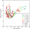 |
Fig. 8. Ratio of explosion energy to ejecta mass inferred using the Mandel & Müller (2020) model as a function of the final mass. The horizontal line at 5 × 1050 erg/M⊙ shows the value of E/M used in Dessart et al. (2020) to produce light curves of Type I SNe. |
However, we highlight that the uncertainties in the predictions of explodability, explosion energy, nickel mass, and remnant mass are more uncertain in BH that form SNe (i.e. fallback SNe) than in explosions that form NS. However, we find that the trends and correlations we present are robust inasmuch as the physical assumptions in our models are robust, but the outcome of our explodability analysis can vary depending on the choice of parameters (see Appendix B). A prediction that is rather robust is that the ejecta masses predicted from our models are found to be larger at low metallicity for a fixed initial mass (since lower metallicity models lose less mass; see Figs. 1 and A.3). Another prediction that may vary quantitatively, but is qualitatively robust, is that the transition between Type Ib and Type Ic progenitors shifts to lower initial helium star masses as metallicity increases. This implies that the maximum mass of the ejecta at which Type Ib SNe are observed will be larger at low metallicities. The maximum ejecta mass at which Type Ic SNe can be observed in different metallicity environments is also expected to decrease at high metallicity, due to the fact that the maximum final mass at which explosions take place decreases with increasing metallicity.
All of these results correspond purely to the outcome of our models, but do not correspond to number of observable events, or the real distribution of SN observables. An estimate of how these distributions will change is estimated in the next section through a simplified population model.
4. Type I supernova and compact object populations
In this section we discuss the properties of Type I SN and compact remnants that result from the simple population synthesis model described in Sect. 2.3. In Sect. 4.1 we present the resulting compact object populations, and in Sect. 4.2 we discuss the resulting distribution of SN observables.
4.1. Compact object populations
The resulting distributions of NS masses, presented in Fig. 9, depend only weakly on the metallicity. We find that the average NS mass is around 1.42 M⊙, but the distributions are skewed towards slightly lower NS masses as the metallicity increases. The distributions resemble the low-mass peak in the millisecond pulsar mass distribution inferred by Antoniadis et al. (2016), but their contribution to the high-mass peak is negligible. These distributions are not affected by our implementation of fallback, but we do not rule out that some massive NS may be formed by late fallback in models where we do not predict it with our formulation. We also find that the lowest-mass NSs in our populations are formed in Type Ib SNe, whereas the most massive components originate in Type Ic SNe, as shown in the lower panel of Fig. 9 (see Fig. A.3). This is due to the correlation between ξ2.5 and the resulting NS mass. Type Ib SNe are produced in models whose final masses are predicted to be below the first compactness peak, and most of them have low values of ξ2.5 due to their smaller final mass. The progenitors of Type Ic SNe, on the other hand, have a larger scatter of values of ξ2.5 since many of them come from models in the region where core carbon burning transitions from radiative to convective, and have a larger scatter in ξ2.5 (Sukhbold & Woosley 2014), and consequently in NS mass. Alternatively, the calculations presented in Appendix B.1 have a few cases where high-mass NSs are produced in low-energy explosions, which probably do not receive sizeable kicks. In this scenario, although rare, these systems may be favourably created in binary systems that statistically are much more likely to stay bound after explosion, therefore biasing the sample of NSs in binary systems.
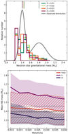 |
Fig. 9. Properties of NS gravitational mass distribution in different metallicities. Top: distribution of NS gravitational masses that result from analysing our core-collapse models with the Mandel & Müller (2020) model, weighted by the IMF from Salpeter (1955), compared to the observed distribution inferred by Antoniadis et al. (2016). The average values of the distributions are represented by vertical lines at the top of the figure. The lowest-mass NSs correspond to progenitors outside of our model grid, and their resulting mass has been assumed to be between 1.22 and 1.3 M⊙. Bottom: Mean value (solid lines) and standard deviation (hatched, shaded regions) of the total distributions and the distributions separated by SN type. The mean value (dashed black line) and the standard deviation (grey line) of the first NS mass peak of the observed distribution of Antoniadis et al. (2016) is shown for comparison. |
The distribution of BH masses that results from our calculations, shown in Fig. 10, has a stronger metallicity dependence. The peak that corresponds to the high-mass BHs, with masses larger than ∼10 M⊙, comes from the models in our grid with the highest initial masses. This peak tends to be at a higher mass for lower metallicities, owing both to the decrease in mass loss and to the decrease in final mass of the location of the threshold between models that form BHs and models that form SNe.
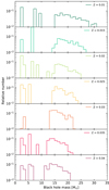 |
Fig. 10. Distribution of BH masses at different metallicities, which results from the analysis of our model with the Mandel & Müller (2020) model, weighted by the IMF from Salpeter (1955). |
The more abundant intermediate mass peak, located at 5–8 M⊙, corresponds to models that form BHs in the first high compactness peak. Given our assumptions on the population, we expect that BHs of this mass should be much more frequent than the high-mass models.
There is a gap between these two regions, also present in the results of other groups (e.g., Ertl et al. 2020; Woosley et al. 2020), but the precise width and location of this gap are found to depend on the metallicity. Extrapolating from our results might suggest that predicting the location and shape of this gap is a difficult (but necessary) effort. The location of this gap at some metallicity may be masked by BHs coming from different environments, so establishing a metallicity behaviour for this gap and convolving it with our knowledge of the metallicity evolution of galaxies of different redshifts is key to properly interpret the observations of BH masses in the Universe, which will become more numerous in the future, with the advent of ongoing and future gravitational wave observatories. Our models also show an apparent dearth of BHs above a maximum mass, but this limit is artificial and corresponds only to the maximum mass of the models in our grid.
Fallback SNe produce a low-mass peak in the distribution, predicted to be around 3 M⊙, and generally less populated than the other two. However, this is sensitive to the number of fallback SNe produced, which may vary in reality. If fallback SNe tend to appear in a certain range of masses, they can create patterns in the distribution of high-mass BHs that manifest themselves as valleys where fewer BHs of a certain mass are found, since they instead inhabit the lowest-mass peak. If this is indeed the case, then the need arises to study this effect in more detail, to be able to better interpret the distributions of BH masses that will become available from future observations of binary BH mergers. The formation of such systems may help explain the asymmetric mergers of compact objects that have recently been detected by the Laser Interferometer Gravitational-Wave Observatory (LIGO) and Virgo collaborations (Antoniadis et al. 2022).
A final trend that is notable in the BH mass distribution is a change in the slope of the BH distribution above a certain mass, also found by Woosley et al. (2020), caused by the change in the implemented mass-loss rate from WN-type mass loss to WC-type mass loss; it corresponds to the change in the trend in the final mass shown in Fig. 1. If this is resolved with the increasing number of gravitational wave sources observed, it could potentially aid in constraining the mass-loss rates of very massive stars.
4.2. Distribution of supernova properties
We present the obtained distributions for ejecta masses, explosion energies, kick velocities, and nickel masses for Type Ib and Type Ic SNe, as cumulative distribution functions in Fig. 11. The observed distributions obtained for Type Ib SNe are shown compared to the observed sample of Type Ib and Type IIb SNe from Taddia et al. (2018), and Type Ic SNe are compared to the previous sample, combined with that of Barbarino et al. (2021), who conducted a similar study focused on Type Ic SNe. We compare our results with observations only after separating them by SN type in hopes that the results of Taddia et al. (2018) and Barbarino et al. (2021) are representative of the distributions of explosion properties of each SN type, but refrain from comparing them with the combined sample, since the observed SN properties do not reflect the relative occurrence of different SN types.
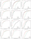 |
Fig. 11. Cumulative distribution functions of ejecta masses, explosion energies, nickel masses, and kick velocities, separated for the full sample of models and separated between Type Ib and Ic SNe that result from analysing our core-collapse models with the Mandel & Müller (2020) model, weighted by the IMF from Salpeter (1955). Different colour lines represent different metallicities. The observed distributions of ejecta masses, explosion energies and nickel masses are drawn from Taddia et al. (2018) for Type Ib, IIb (grouped with Type Ib), and Ic SNe, and additionally from Barbarino et al. (2021) for a larger sample of Type Ic SNe. The average values of each distribution are indicated with vertical lines at the top of each panel. |
Many trends become apparent in our estimation of the distribution of SN observables. The predicted distribution of the ejecta masses of Type Ic SNe resembles the distributions we obtain at high metallicity, but the metallicity range that likely corresponds well with the observed distribution is much too high to explain most Type Ic SNe. We also find that, regardless of the metallicity, no Type Ic SNe are produced within our models with ejecta masses lower than about 2 M⊙.
The predicted distribution of the ejecta masses of Type Ib SNe is skewed to considerably lower values than the observations. These results, however, have been taken at face value from the outcome of our stellar evolution tracks, and many of them overestimate the mass-loss rates of the progenitors of Type Ib SNe, since they have luminosities below  . To remedy this, we repeat our calculation using the initial mass as a better proxy of the final mass, but retaining the same distribution of NS masses. This results in the distribution shown in Fig. 12, which yields a better fit to the data.
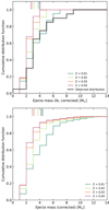 |
Fig. 12. Cumulative distribution of ejecta masses for Type Ib SNe (top) and for all stripped-envelope SNe (bottom) that result from our models, but corrected for the strong variation in wind between WR stars and low-mass helium stars. Here, ejecta masses for stars with initial mass above the minimum mass of WN-type stars are drawn from our model results, and for the rest we assume no mass loss, but the same NS mass as predicted from its original model. |
As expected, we find that the ejecta masses of stripped-envelope SNe, both in Type Ib and Type Ic, decrease as the metallicity increases. As shown by the mean values and standard deviations of the distributions in Fig. 13, the ejecta masses for both types of SNe decrease dramatically as a function of metallicity, but even by applying a correction for the progenitors of Type Ib SNe with very low mass, the range at which these events are found cannot be reproduced from our models.
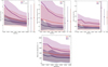 |
Fig. 13. Mean values (lines) and standard deviation (shaded region) of the ejecta masses, explosion energies, nickel masses and kick velocities of model populations, obtained by analysing our core-collapse models with the Mandel & Müller (2020) model, weighted by the IMF from Salpeter (1955). These values are shown for the total population of stripped-envelope stars (orange), as well as separated into Type Ib (violet) and Type Ic SNe (blue). For comparison, the mean values and standard deviations of the ejecta masses, the explosion energies, and the nickel masses inferred from the samples of Taddia et al. (2018) and Barbarino et al. (2021) are shown on the right. |
We find that the average explosion energies estimated for our models range between about 1.3 and 1.8 × 1051 erg. We find that this average decreases as a function of metallicity. The average values of Type Ib SNe tend to be below the observed average energy at every metallicity, whereas our Type Ic SN models have larger average energies than the observed samples. The explosion energies of Type Ib SNe vary relatively little as a function of metallicity, whereas those of Type Ic SNe tend to decrease quite drastically with increasing metallicity. The energies estimated for Type Ib SNe are considerably lower, but we have not corrected for these values for the different wind-mass-loss rates for low-mass helium stars. The energies predicted for Type Ic SNe at high metallicity agree well with the observed values, although the number of explosions below 1051 erg is underestimated.
We find that the amount of 56Ni synthesised in SNe decreases as the metallicity increases. The distributions of the 56 Ni mass peak around 0.05 M⊙ and there are few cases with nickel masses higher than 0.1 M⊙. For both SN types, we find that the amount of nickel synthesised during the explosion decreases with increasing metallicity. The values we find are systematically lower than the observed values, which also have a much broader distribution, and are found to have closer to 0.15 M⊙ of nickel on average.
The distribution of kick velocities obtained from our models peaks at around 300–400 km s−1, and we find that kick velocities tend to decrease with increasing metallicity. We also find that Type Ic SNe tend to produce SNe with kicks considerably larger, on average, than those coming from Type Ib SNe.
Except for the emergence of a new, low-mass peak in the BH mass distribution, fallback SNe are found to be too rare to have a perceivable effect on the distribution of SN observables in large samples. This happens because these events predominantly originate in very high-mass stars, which are therefore very rare.
Another immediate consequence of the metallicity dependence of stellar winds is an increase in SNe Type Ic rates with respect to SNe Type Ib for higher metallicity. We estimate the number ratio of Type Ic SNe to Type Ib SNe as a function of metallicity and find that it is strongly metallicity dependent, as shown in Fig. 14.
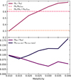 |
Fig. 14. Number ratios of different quantities as a function of metallicity, as obtained from our model population. Top: number ratio of Type Ib SNe to Type Ic SNe, ⟨NIc/NIb⟩, compared to the observed ratio of Type Ib SNe to Type Ic SNe ⟨NIc/NIb⟩obs and of Type Ib SNe plus Type IIb to Type Ic SNe ⟨NIc/(NIb + NIIb)⟩obs in the local Universe, inferred from the relative rates of Shivvers et al. (2017). Bottom: Number ratio of BHs to SN explosions ⟨NBH/NSN⟩ and number ratio of Type Ib SNe with WR progenitors to Type Ib SNe with transparent-wind helium star progenitors ⟨NIb from WR/NIb from TWHS⟩. |
According to our models, the number ratio of Type Ic to Type Ib SNe should increase as a function of metallicity, starting from approximately 0.2 at a metallicity of 0.01, to about 0.7 at a metallicity of 0.04. This rising trend is mainly due to the fact that the initial helium mass threshold for the production of a Type Ic SN decreases with increasing metallicity. We compare our calculation to the observed ratio of stripped-envelope SNe using the observed rates of different types of SN in the local Universe from Shivvers et al. (2017). We find that the value estimated from our models around solar metallicity is between the observed ratio of Ic to Ib in the local Universe, which represents an upper limit to our model; and the ratio of Type Ic SNe and the rest of stripped-envelope SNe (Types Ib and IIb), which is a more realistic quantity to compare our results to.
Two final quantities that we derive from our population model and present on the right y axis of Fig. 14 are the relative ratio of BHs to SNe and the relative ratio of Type Ib SNe that have WR-type progenitors to those that have transparent-wind helium stars as progenitors (i.e. stars that have luminosities below  ). We find that as metallicity increases, the number of massive stars that produce BHs tends to decrease. At a metallicity of 0.01, we find that around 16% of massive stars produce BHs, whereas the number decreases to about 8% in the metallicity range 0.025–0.04. This is due to the reduction in final mass as a function of initial helium star mass (see Fig. 1), combined with the location of the islands of explodability (see e.g., Fig. 5). On the other hand, as metallicity increases, the number of Type Ib SNe that have WR stars as progenitors tends to increase. This result is non-trivial because even though the minimum luminosity at which we expect stripped-envelope stars to be WRs decreases as a function of metallicity, so does the minimum luminosity at which our models produce WC-type stars, meaning that even though there are more WN-type stars at lower luminosities, the threshold at which they explode as Type Ic SNe also decreases. In the metallicity range of our models, this number tends to increase, but the behaviour is likely different in metallicities beyond those in our grids. However, the absolute value of this ratio at all metallicities in our grid is below 18%, implying that most Type Ib SNe originate from low-mass helium stars with transparent winds, and not WR stars. The number is likely to be even lower at metallicities corresponding to environments like the SMC and below, and this trend should be reflected in the methods that are employed in the search of direct imaging of Type Ib SN progenitors.
5. Discussion
The results presented in this work were derived from evolutionary calculations of helium stars with metallicities in the range 0.01–0.04, and their resulting core-collapse models. The aim of studying helium stars in this metallicity range is to explore a possible evolutionary channel that can help explain the observed prevalence of Type Ic SNe in high metallicity environments (Modjaz et al. 2011), and to address the discrepancy between the predicted final masses of stripped-envelope SN progenitors (e.g., Woosley et al. 1993; Meynet & Maeder 2005; Yoon et al. 2010; Georgy et al. 2012), and the distribution of ejecta masses observed in SNe, particularly of Type Ic (e.g., Taddia et al. 2018; Barbarino et al. 2021).
We divide our core-collapse models into possible progenitors of either Type Ib or Type Ic SNe according to whether their surface has a helium abundance of Y = 1 − Zinit and high nitrogen abundance, or whether it has decreased helium abundance and is instead enriched with the products of helium burning, respectively. This dichotomy has been found to be at the heart of the differences in the spectral characteristics of Type I core-collapse SNe by Dessart et al. (2020).
We then analysed our results according to the explodability tests of O’Connor & Ott (2011), Ertl et al. (2016), and Müller et al. (2016), the last of which includes the effect of fallback following Mandel & Müller (2020). Their explodability test consists of a parameterised, semi-analytical model of the explosion, which yields predictions of NS gravitational masses, ejecta masses, and nickel masses in successfully exploding models. We also estimate the distribution of kick velocities following Mandel & Müller (2020). Finally, we construct a simple synthetic population of stripped-envelope SNe to contrast our results with observations.
In this section we discuss and interpret the results obtained from analysing our core-collapse models and the resulting population, as well as the uncertainties that might have an impact on our results.
5.1. Uncertainties in core-collapse stellar models
Some uncertainties in our models are inherent to our physical and numerical assumptions, and others stem from poorly constrained physical parameters. Many are discussed in detail in Paper I, but here we list some, paying particular attention to those that affect our models at core collapse.
5.1.1. Uncertainties in the mass at core collapse
Our evolutionary calculations are modelled using the empirical mass-loss rates suggested by Yoon (2017). However, stars with luminosities below  are believed to lose mass at a much lower rate. The precise mass-loss rates of these stars are unknown, but the simulations of Vink (2017) suggest that the mass-loss rates of such stars are orders of magnitude below those of WR stars.
Since we extrapolate WR mass-loss rates into this regime, the final masses of models with luminosities below  are overestimated. Furthermore, the core evolution of these models does not correspond to that of helium stars of the appropriate final mass. This probably has no effect on whether they explode or not, since models with luminosities below
  have low initial masses and are expected to have low values of ξ2.5, leading to successful SN explosions. The approach we take to overcome this limitation in our population models is to assume that the helium stars that produce SNe in this regime have final masses that can be approximated by their initial masses, since they have very low mass-loss rates. We further justify this assumption a posteriori arguing that this makes our estimates for the ejecta masses resemble the observed distribution more closely. For these stars, we assume that the NS gravitational mass is 1.22–1.3 M⊙, and we assume that the minimum mass at which stars explode as SNe is 3 M⊙, following Chanlaridis et al. (2022).
The mass-loss rates of WR stars are also uncertain. Recent theoretical estimates of WR winds (Sander et al. 2020; Sander & Vink 2020) suggest that WR winds have a weaker dependence on metallicity and that the WC star mass-loss rates are lower than the empirically obtained values of Tramper et al. (2016). This would imply that the final masses of WC stars in our models are underestimated, as well as those of models with high Z.
The masses of our models at core collapse may also be overestimated due to the implementation of MESA’s mlt++, which enhances the efficiency of energy transport by convection, and results in more compact stars that show very little or no envelope inflation (e.g., Sanyal et al. 2015). The mass-loss rates of WR stars should not be affected by this assumption since they only depend on the luminosity and metallicity of helium stars, which are well constrained by our models. However, if they exceed the Eddington limit in their envelopes by a large amount, it can lead to episodic mass loss (e.g., Owocki 2015). Furthermore, if inflation causes helium stars to expand significantly beyond their initial radius, it might trigger a second episode of mass transfer with their companion, which will also reduce their final mass.
Another uncertainty in our models comes from ignoring the main-sequence and envelope stripping phases, and modelling directly fully stripped helium stars. As discussed in detail in Paper I, envelope stripping is not always efficient in removing all hydrogen from the surface of a star. Therefore, they are likely to spend a fraction of their helium-burning lifetime with a hydrogen envelope of varying mass, which can result in higher final and ejecta masses than those predicted in our models.
5.1.2. Uncertainties in the core structure
In addition to the uncertainties introduced in our modelling by ignoring the main sequence evolution of the progenitors of stripped-envelope stars and by their mass-loss rates; other issues affect the accuracy of numerical simulations of massive star evolution, which are not unique to helium stars, but affect stellar evolution models in general. Numerical resolution and the choice of nuclear network are known to lead to different core structures in core collapse, which, in turn, may affect the explodability of stellar models (Farmer et al. 2016). We used a nuclear network with only 21 isotopes, which led to uncertainties in the final core structure of our models. We made this choice for practical reasons, since we wanted to cover a large mass-and-metallicity parameter space. We argue that, while the exact masses at which models transition from convective to radiative nuclear burning is uncertain due to our choice in nuclear network, our calculations seem to be in broad agreement with those of other works, where simulations with larger nuclear networks are performed (e.g., Sukhbold & Woosley 2014; Sukhbold et al. 2018; Ertl et al. 2016; Laplace et al. 2021; Farmer et al. 2020; Schneider et al. 2021), in particular on the morphology of the compactness parameter ξ2.5 as a function of final mass (see Fig. 5). Furthermore, they cover a broad enough range that this uncertainty will likely not affect the main conclusions we draw from our results. However, although we expect that the global properties we infer are robust, we highlight that simulations with larger nuclear networks are a complicated, but necessary test to confirm the predictions made in this paper, in particular those that concern the explodability of individual models.
The efficiency of the 12C(α,γ)16O reaction in particular remains uncertain (deBoer et al. 2017), and can have a large effect on the evolution and outcome of stripped-envelope stars, as it may influence the amount of carbon remaining at the end of helium burning, which in turn influences whether carbon burning proceeds radiatively or convectively (Imbriani et al. 2001). This is known to have a large effect on the explodability of massive stars (Sukhbold & Woosley 2014; Patton & Sukhbold 2020; Schneider et al. 2021), as well as on the upper limit for BH formation (Farmer et al. 2019, 2020). The effect of these uncertainties is beyond the scope of this work, but they can have an effect on the exact predictions of our analysis. However, we argue that because of the size of our model grids, the effect of metallicity-dependent mass loss on the evolution of helium stars explored in this work will have a larger impact than that of the uncertainties inherent to stellar evolution models.
The efficiency of convection and the presence of overshooting in helium stars are also uncertain. Varying these parameters may lead to convective helium-burning cores of different mass. This will result in different lifetimes and lead to significant differences in evolution, particularly in the lower-mass regime. Overshooting in low-mass helium stars will most significantly affect the locations of the boundaries in initial mass that lead to different final outcomes Chanlaridis et al. (2022). This uncertainty is perhaps the largest in our population models, as it might imply that the minimum mass at which stars become core-collapse SNe is dependent on metallicity. We believe that variations in this limit will likely have an effect on real populations of stripped-envelope SNe, but the conclusions derived from our simplistic model will remain broadly valid. However, we highlight the need for a more detailed population synthesis model of stripped-envelope stars, which additionally includes the efficiency of stripping as a function of both mass and metallicity.
5.1.3. Determination of supernova properties
Using the Müller et al. (2016) SN explosion model, we estimate the properties of the resulting explosions of individual models. These properties are relatively uncertain on their own, and accurate estimations of the explosion outcome can only be more accurately determined through detailed 3D simulations. However, this model can produce predictions on much shorter timescales and predicts trends in the behaviour of large sets of models, revealing the consequences of the assumptions made to produce them. These explosion models, however, depend on a series of free parameters (see Sect. 2, and Appendix B) and variations in their value produce different results.
We have performed several tests to characterise the effect of variations in these parameters. We find that, within a reasonable range of values, the result of the models is broadly similar. The distributions produced by simulating SNe explosions with a different set of parameters change the individual values of the predicted outcomes and the range where explosions are expected to occur, so we chose the set of parameters that more closely resembles the predictions of the Ertl et al. (2016) explodability test.
5.2. Comparison to previous stellar evolution models
Numerical studies to investigate evolutionary channels for the progenitors of stripped-envelope SNe have been carried out extensively in the context of single star evolution (e.g., Meynet & Maeder 2003; Georgy et al. 2009, 2012; Chieffi & Limongi 2013), massive stars in binaries (e.g., Podsiadlowski et al. 1992; Yoon et al. 2017; Schneider et al. 2021; Laplace et al. 2021), and through the evolution of helium stars (e.g., Dessart et al. 2020; Ertl et al. 2020).
Single-star models where wind stripping is the only component that produces hydrogen-free stars at core collapse require very large initial masses (≳25 M⊙), which may be in conflict with the rate of stripped-envelope SNe, and predict high final masses, which is in conflict with the observed distribution of ejecta masses (e.g., Yoon 2015). Binary stellar models are much less restrictive in the minimum mass that is required to produce stripped-envelope stars, but often grids of binary models have very few suitable progenitors for Type Ic SNe (e.g., Yoon et al. 2010, 2017).
Yoon (2017) suggested that modifying the mass-loss rates of WR stars could contribute to producing models in the right mass and composition range, and these models were found to reproduce the spectral properties of Type Ib and Type Ic SNe by Dessart et al. (2020). The models in this work have properties and evolution very similar to those of Dessart et al. (2020), but extend the applicability of their predictions by covering a larger range of mass and metallicity and analysing their explodability properties.
We find that the core properties of our models at core collapse are consistent with previous models of stripped-envelope stars coming from binary calculations, and – like other single helium star models (e.g., Woosley 2019; Ertl et al. 2020) – form a distinct family of transient progenitors with properties that differ from those obtained for single stars: stripped-envelope stars tend to have lower compactness, lower central carbon mass fraction at the end of helium burning, and lower carbon-oxygen core masses than stars with similar main sequence masses that did not become stripped (Woosley 2019; Laplace et al. 2021; Schneider et al. 2021).
Studying several metallicities, however, allows us to isolate the effect of mass loss in the core and surface properties of helium stars. We find that the effect of distinct mass loss in the WN and WC phases can have a strong effect on the pre-collapse properties of WR stars. Most notably, we find features that were either absent or not reported in previous models: compactness parameters of helium stars with final masses above ∼16–25 M⊙ bifurcate, creating two families of solutions that have typical compactness parameters of ∼0.4–0.6 and ∼0.6–0.8. Explodability tests (O’Connor & Ott 2011; Ertl et al. 2016; Müller et al. 2016) predict these models to form BHs with approximately the final stellar mass, but using the model of Mandel & Müller (2020), we find that many of the low-compactness models are candidates for forming fallback SNe (i.e. a fallback island of explodability). These models may be similar to successfully exploding models of M > 60 M⊙ of Ertl et al. (2016), but the connection between them and the reason for the bifurcation are unclear.
5.3. Transients and compact objects
5.3.1. Explodability of stripped-envelope stars
We find that the distribution of ξ2.5 is similar for helium stars of different metallicities that have similar final masses. However, differences between the distributions of ξ2.5 as a function of final mass probably arise due to differences in CO core masses and central carbon abundances at the end of helium burning and result in variations in the core structure. These discrepancies are reflected in the different values of M4 and μ4 that we find for stars of similar final mass, as well as in the results obtained from applying the Müller et al. (2016) and Mandel & Müller (2020) model to our stellar models at core collapse (see Fig. A.3).
The difference in core structure in models of equal final mass implies that the ejecta mass and remnant mass distribution at different metallicities will be affected by more than just a displacement in the final mass distribution of models (see Figs. 6 and 7). The imprint of these differences is summarised in Figs. 11 and 10, and is further discussed below.
5.3.2. Ejecta masses of stripped-envelope supernovae
Many of our predictions are agnostic to the assumptions and uncertainties inherent in the SN model. In particular, the masses of models that explode or implode are in agreement with the predictions obtained from the Ertl et al. (2016) test. This suggests that the distributions of BH masses and of SN ejecta masses are roughly independent of the way they were obtained and reflect only the metallicity dependence of the WR mass loss.
We find that the distribution of ejecta masses for Type Ic SNe is reproduced by our models, preferentially at very high metallicity (0.03–0.04). This suggests several interesting possibilities for the progenitors of these SNe. Modjaz et al. (2011) found that most Type Ic are indeed produced in environments of super-solar metallicity, but it is unlikely that the typical metallicity of their progenitors is twice solar and higher. Instead, this might reflect that the mass-loss rates inferred for WN-type stars, WC-type stars, or both are higher than what is reported in the literature, in stark contrast with the predictions of Sander et al. (2020) and Sander & Vink (2020).
Another possibility is that stripped-envelope stars experience short episodes of mass loss at the end of their lives, likely originating from their proximity to the Eddington limit. Another explanation is that, since many of them are likely to be formed in binaries, they may experience episodes of mass transfer after they have been stripped and therefore reach the end of their lives with lower masses. Because helium stars lose mass at such a high rate, both their radii and their luminosities decrease during their core helium-burning lifetime. This implies that even if they are in a close binary, helium stars will not interact with their companions during core helium burning and can only interact in later stages if helium shell burning drives a radial expansion.
We also find that the ejecta masses of our models, even at the highest metallicities in our grid, fail to reproduce the lowest observed ejecta masses. This phenomenon could be explained by the reasons stated above, or it could be caused by a larger fraction of their progenitors experiencing late-time fallback during explosion, leading to the formation of massive NSs or low-mass BHs and low-mass ejecta explosions (although fallback SNe are not predicted in the relevant mass regime by Ertl et al. 2020, but see Vigna-Gómez et al. 2021 and Appendix B).
The observed distribution of Type Ib SNe is closer to the results of our models at low metallicity, but the predicted distributions of ejecta masses for Type Ib SNe obtained by taking the output from the models at face value are overestimated. Helium stars with initial masses below or near the minimum mass at which stripped-envelope stars are observable, because WN-type stars lose less mass than their WN counterparts. Through our simplistic population model, we find that most progenitors of Type Ib SNe will in fact not be WR stars, but rather helium stars with transparent winds that lie below this limit. We propose this as an explanation for the stark discrepancy between the ejecta masses of Type Ib SNe predicted from our models and the observed sample from Taddia et al. (2018), who find Type Ib SNe with significantly larger ejecta masses than those that result from our models, and find that correcting for this produces a distribution of ejecta masses that is more similar to the observed distribution. However, Type Ib SNe progenitors that come from stars that are stripped of their hydrogen envelope after a significant fraction of their helium-burning lifetimes have taken place may also contribute to increasing the number of Type Ib progenitors with high ejecta mass and to increasing the scatter in the distribution.
5.3.3. Explosion energies, nickel yields, and kicks
The values predicted for SN explosion energies, nickel yields, and kick velocities from our helium star models rely on the Müller et al. (2016) model. We calibrated the input parameters of the model to agree with the predictions of the explodability test of Ertl et al. (2016) and to produce explosion energies and values of E/M in a range that we found reasonable.
For many models, we find explosion energies that are larger than those predicted by the more detailed study of Ertl et al. (2020), even when only neutrino-driven explosions are considered. However, recent 3D simulations of SN explosions from massive progenitors (e.g., Powell & Müller 2020) have found that the production of SNe with energies in excess of about 3 × 1051 erg is plausible. The highest energies in our models come from fallback SNe. The models in which we predict the fallback SNe to take place are typically of higher mass, so a larger energy is required to unbind the envelope of the progenitor. As the fallback prescription of Mandel & Müller (2020) has been calibrated based on 3D fallback simulations of relatively weak explosion, the extrapolation to the very energetic fallback SNe predicted in this study is quantitatively uncertain, and the largest explosion energies, which well exceed any 3D models of neutrino-driven models, may be overestimated. On the other hand, late-time fallback accretion provides an additional energy source that allows explosions to occur even after the central proto-NS has reached its maximum mass. This is not included in our analytical treatment.
Furthermore, the nickel masses in fallback explosions are more uncertain than the energetics. Whereas the transfer of energy from the engine to the ejecta in a fallback explosion can be approximated analytically in a quasi-spherical picture, the amount of Ni that survives fallback will depend sensitively on mixing instabilities, for which we presently do not have an effective treatment in our analytic SN models.
Regardless of the high energies that some individual models reach, the predicted distribution of energies in our population models does not contain many of these very high energy explosions, as they originate predominantly in high-mass models. The energy distribution we obtain for Type Ib SNe at Z = 0.01 seems to be in rough agreement with the observed sample of Taddia et al. (2018), although it is skewed to slightly lower energies (see Fig. 11). A possible explanation for this behaviour might be that the progenitor mass of the majority of our models is underestimated, since they correspond to helium stars below the minimum WN luminosity limit. A larger final mass will result in larger carbon-oxygen core masses at core collapse, which is, in turn, likely to shift the distribution to higher energies. Furthermore, progenitors of Type Ib SNe that come from stars that were not fully stripped after the main sequence may also result in more energetic explosions since they are expected to have higher final mass and higher core mass. This conjecture can be tested when accurate progenitor models of Type Ib SNe become available.
The energy distribution of Type Ic SNe, on the other hand, has the opposite effect. Since most of the progenitors of Type Ic SNe at low metallicity come from stars of higher mass (and are also, therefore, rarer), the energy distribution we obtain is skewed to much larger energies. It is only at higher metallicity that we find a broad energy distribution that also includes lower-energy explosions and resembles the observed distribution more closely.
Like ejecta masses, explosion energies of Type Ic SNe are only reproduced by very high metallicity models, and even at our highest metallicity, we find that the SNe with the lowest kinetic energies in the observed sample are missing from our predictions. This supports our claim that Type Ic SN progenitors likely experience additional mass loss, either as a result of winds or a different effect that acts on shorter timescales.
However, it should be noted that the masses of ejecta and the explosion energies inferred from the light curves of stripped-envelope SNe are degenerate (i.e. several combinations of these two parameters can produce identical light curves; see Dessart et al. 2020). However, comparing the value of E/Mej predicted by our models with the observed result in a distribution that is similar to those obtained in observations. However, we note that there is a large scatter in the value of E/Mej that results from our models. The distribution of this quantity ranges from about 0.3 × 1050 erg/M⊙ in models with the lowest masses, monotonically increasing with initial mass up to about 2 in the models with the highest initial mass, while some models with initial masses in the range of 20–40 M⊙ reach slightly larger values, as well as those that are predicted to become fallback SNe.
Nickel masses in our models tend to be considerably lower than those found by Taddia et al. (2018) and Barbarino et al. (2021) at every metallicity. Our population model predicts that the median nickel mass of Type Ib SNe is about a factor of 3 lower than that of the analysed sample. In Type Ic SNe, the difference is less stark, about a factor of 2, but is still widely underestimated. We find that the nickel mass has a tendency to decrease with the metallicity.
The nickel mass in the observed samples is obtained by means of Arnett’s rule (Arnett 1974). This estimate has been found to overestimate the nickel mass produced in SNe stripped envelopes of all types (Dessart et al. 2016; Afsariardchi et al. 2021), which may help explain the discrepancy between our estimations and the observed sample. As with explosion energies and ejecta masses, in the case of Type Ib SNe, an additional cause for the prediction of low nickel masses might be that their final mass is underestimated, since we find that most Type Ib SNe originate in stars with luminosities below the minimum WR luminosity and, therefore, have overestimated mass-loss rates.
Kick velocities are computed following Vigna-Gómez et al. (2018). They depend on the explosion energy and the remnant mass (as well as in the mass enclosed between the acceleration region and the point where the shock exceeds the escape velocity of the material below it) and are therefore correlated (see Fig. A.3). The distribution of kick velocities in our models is similar to that of Mandel & Müller (2020) and is similar to the velocity distribution of pulsars (Hobbs et al. 2005). However, we find that the distribution has a tendency to decrease with increasing metallicity, probably as a consequence of the decrease in the mass of SN progenitors.
5.3.4. Neutron star and black hole mass distributions
We find that Type Ic SNe produce more massive NSs than Type Ib SNe. In agreement with Ertl et al. (2020) and Schneider et al. (2021), we find that NS gravitational mass is correlated to ξ2.5 (see Fig. A.3). This implies that the prediction is also independent of the SN explosion model, since most Type Ic progenitors come from stars that are more massive than those of Type Ib SNe at the time of core collapse, and also tend to have a higher value of ξ2.5.
Variations in the location of the islands of explodability as a function of metallicity are clearly reflected in different BH mass distributions. Our results resemble those of Woosley et al. (2020), but we find that variations in metallicity result in more drastic changes in the locations of the peaks and valleys of the BH mass spectrum.
The emergence of a low-mass peak at around 3 M⊙ in some of our grids arises from fallback SNe that result from some high-mass models with relatively low values of ξ2.5. The intermediate mass peak in our distributions is displaced from around 9 M⊙ at Z = 0.01 to around 6 M⊙ at Z = 0.04 and has a structure that results from variations in the properties of the core as a function of mass in models in this regime, consequence of the transition between carbon burning in the convective and radiative core (Sukhbold & Woosley 2014).
The peak mass in the distribution that corresponds to high-mass BHs, above 10 M⊙, also decreases as a function of metallicity. Due to variations in explodability that arise as a function of metallicity, even in models with the same final mass, it is enough to bring this peak from about 15 M⊙ in the Z = 0.01 grid, down to about 11 M⊙ at Z = 0.04. The highest-mass BH at each metallicity corresponds to the highest-mass model and does not carry information on whether the location of the BH mass gap depends on the metallicity.
This behaviour reflects the need to take the metallicity dependence of BH mass production into account when generating predictions for the BH mass distributions in the Universe and when interpreting the findings of the LIGO and VIRGO collaborations (e.g., Acernese et al. 2015; Fishbach et al. 2021) and future gravitational wave observatories.
5.3.5. The metallicity evolution of progenitors of stripped-envelope supernovae
We find that the number ratio of Type Ib SNe to Type Ic SNe increases as a function of metallicity because of the metallicity-dependent mass-loss rates of WR stars. Our findings are in general agreement with the relative rates found in the local Universe (Shivvers et al. 2017), and with the fact that Type Ic SNe are found in environments of higher metallicity than other core collapse SNe (Modjaz et al. 2011). According to our analysis in Paper I, stars in our sample that evolve to become progenitors of Type Ic SNe will be luminous enough to be observable as WC-type stars, meaning that they are unaffected by the uncertainty in the mass-loss rates of low luminosity helium stars.
However, we find that although the relative number of Type Ib SNe with transparent-wind stripped-envelope stars as progenitors relative to those that have WR progenitors both tends to increase as a function of metallicity, it is below 0.2 even at the highest metallicity in our grid and about 0.06–0.08 at approximately solar metallicity. Even though the value of the minimum luminosity of WR stars as a function of metallicity is approximate, this implies that, in our simplistic model, the overwhelming majority of progenitors of Type Ib SNe are, in fact, not WR stars, but rather stripped-envelope stars with transparent winds and luminosities below the WR threshold. This result is further backed by the fact that, making this assumption, the distribution of ejecta masses we obtain for Type Ib SNe resembles the observed distribution more closely.
Because all of our explodability tests roughly coincide in their results, the inferred values of ratios presented in Fig. 14 are independent of our SN calculations, and their uncertainties stem from uncertainties in our determination of the minimum WR luminosity, the minimum mass at which helium stars produce core-collapse SNe, and the stripping efficiency of stars as a function of metallicity.
The number of SNe coming from low luminosity helium stars is not expected to be affected by a reduction in the mass-loss rate of their progenitor, since their low initial mass also implies a low value of ξ2.5. Therefore, we argue that our calculations on the relative rate of SN types and the spectral class of the progenitors of Type Ib SNe (Fig. 14) are not dependent on the effect of decreasing winds for helium stars with luminosities below the minimum WR luminosity, but they are uncertain, as the minimum WR luminosity and the minimum mass at which stars produce SNe are uncertain.
Although WR stars are not very luminous in optical bands, since they are compact and hot, the problem becomes more dramatic for low-mass stripped-envelope stars, as they do not show strong emission lines and are less luminous and comparably compact. The fact that we predict that most Type Ib SNe form in transparent-wind helium stars could be the reason why many searches for archival images of their progenitors at SN explosion sites have been unfruitful (e.g., Smartt 2009). During the core-helium-burning phase, low-mass helium stars with transparent winds are not very bright in optical wavelengths (Götberg et al. 2018), where searches for their progenitors have taken place. Models predict that, below a certain mass, helium stars expand during the late phases of their evolution. This expansion is caused by a combination of inflation and the presence of a helium-burning shell (e.g., Yoon et al. 2010; Woosley 2019). This implies that the temperatures of helium stars after core helium depletion will decrease, leading to a larger brightness in the optical band (Yoon et al. 2012; Kim et al. 2015). The transition mass at which expansion becomes important cannot be directly assessed from our models, since it requires a more detailed treatment of the envelope (i.e. without the use of mlt++). However, our current models indicate that this is metallicity dependent and may have consequences for the fate of these stars, particularly if they are in binaries (Yoon et al. 2010; Vigna-Gómez et al. 2021).
Direct observations have been so far limited by the fact that most of these explosions have not been detected in the nearby Universe. Regardless, new atmosphere and stellar evolution models of low-mass stripped-envelope stars are required to constrain their properties at core collapse. Their mass-loss rates and the response of their envelopes to expansion (both due to inflation and helium shell burning) as a function of metallicity are paramount for understanding current and future identifications of progenitors of Type Ib SNe and currently available upper limits on their optical brightness. Together with direct observations of stripped-envelope stars, this may reveal phenomena that occur in the final few thousand years of the evolution of stripped-envelope stars, which are so far poorly constrained.
5.4. Implications for double compact object assembly and gravitational wave sources
Massive binaries are believed to be the progenitors of double compact object mergers and gravitational wave sources. Furthermore, massive binaries that interact are believed to be common in the field (e.g., Sana et al. 2012), and these interactions usually result in mass transfer episodes and subsequent envelope stripping (e.g., Bhattacharya & van den Heuvel 1991; Tutukov & Yungelson 1993; Belczynski et al. 2016). Additionally, wind stripping can also occur in massive binaries, particularly at high metallicities (e.g., Georgy et al. 2012). Therefore, the evolution of stripped helium stars plays a fundamental role in the assembly and characterisation of double compact objects.
5.4.1. Compact object formation and islands of explodability
The predictions of the properties of a compact object remnant is a difficult problem. The main question, in the context of gravitational wave sources, is what the mass of a remnant is given a stellar progenitor. Although for decades the answer seemed to be that increasing masses lead to increased remnants (e.g., Fryer et al. 2012), more recent and more detailed studies suggest that the structure of the star at core collapse plays a crucial and complex role (e.g., O’Connor & Ott 2011; Ertl et al. 2016, 2020; Patton & Sukhbold 2020). One of the main features that has emerged from the discovery of ‘islands of explodability’ can be interpreted as models that are similar in mass at core collapse but lead to significantly different compact object remnants, the most extreme case scenario being a light NS and a heavy BH. Additionally, it represents regions in the progenitor mass space that are very discontinuous in the remnant mass space. According to our results, the picture may be further complicated by the presence of fallback SNe resulting from the evolution of very massive stars (see Fig. A.2), which lead to the formation of remnants with very small masses. This probably has important implications for the rates of double compact objects. If these islands of explodability are real (i.e. not a numerical artefact), that would decrease the rates of binary BH mergers and likely increase the rate of NS–BH mergers (modulo disruption via NS natal kicks).
Double compact object mergers with highly asymmetric mass ratios, such as the ≈23.0–2.6 M⊙ gravitational wave event GW190814 (Abbott et al. 2020), might be the right candidates to probe the explodability island hypothesis. Currently, rapid population synthesis models struggle to predict such asymmetric mergers (e.g., Zevin et al. 2020), even when considering the possibility of explodability islands (Mandel et al. 2021). This idea is further explored by Antoniadis et al. (2022).
5.4.2. High-mass X-ray binaries
High-mass X-ray binaries are observed systems that can potentially become double compact objects. The outbursts of Be X-ray binaries (e.g., Rappaport & van den Heuvel 1982), composed of Be stars (e.g., Rivinius et al. 2013) and a compact accretor, have been observed in the Milky Way and Magellanic Clouds (Reig 2011). The compact object progenitor is believed to have been stripped in a mass transfer episode with the stellar companion (e.g., Vinciguerra et al. 2020), and therefore probably spends a fraction of its lifetime as a stripped-envelope star. Its behaviour will be determined by whether or not its luminosity is above the minimum WR luminosity (i.e. if it is a WR star or not). Furthermore, the presence of inflation will determine whether binaries that include a stripped-envelope star will have episodes of accretion, and the question remains whether this accretion will be stable or lead to a merger.
If the star in an X-ray binary is indeed a WR, its winds are expected to widen the orbit. Moreover, higher mass-loss rates, as those expected at higher metallicities, lead to longer period orbits. Heavier X-ray binary systems are composed of O-type stars with BH companions, which have been the archetype of interacting compact object binaries since the discovery of Cygnus X-1 (e.g., Bowyer et al. 1965; Webster & Murdin 1972; Bolton 1972). Recently, the inferred BH mass of Cygnus X-1 has been corrected from 14.8 M⊙ to 21.2 M⊙ (Miller-Jones et al. 2021), suggesting that winds from massive stars at high metallicities have been overestimated in the last decades. The canonical evolutionary pathway in the formation of Cygnus X-1 involves a helium star with a stripped (initial) mass between 22 − 30 M⊙, depending on the metallicity (Neijssel et al. 2021).
Having a better understanding of the evolution of stripped-envelope stars is essential to understanding the observable time of X-ray binary progenitors as WR stars (van den Heuvel et al. 2017), the evolution of the orbit and assembly of the X-ray binary phase (e.g., Repetto et al. 2017), and the fate of the system as a double compact object (e.g., Klencki & Nelemans 2019). The results presented in this paper and in Paper I show that metallicity, WR winds and inflation can significantly alter the evolution of stripped-envelope stars, and consequently the populations of X-ray binary systems that contain them. Future work should focus on the effect of winds and inflation on the evolution of such systems, which have been found to have different properties as a function of metallicity (e.g., Kouroumpatzakis et al. 2021).
5.4.3. Gravitational wave sources
Most double compact objects formed in isolation are expected to participate in at least one mass transfer episode throughout their evolution. The canonical binary BH formation scenario from isolated binaries includes stripping via the common envelope phase (e.g., Belczynski et al. 2016; Stevenson et al. 2017). However, more recent studies suggest that stable mass transfer might be frequent during binary BH formation (Neijssel et al. 2019; Marchant et al. 2021). The details of stripping are complex and not well understood (e.g., Vigna-Gómez et al. 2022), but it is not unreasonable to expect that stripped stars will (eventually) be stripped-envelope stars. The fate of a binary system is deeply entangled with the evolution of stripped helium stars. The post-stripping radial evolution dictates whether or not they will engage in an additional mass-transfer episode, as well as if they can merge within the age of the Universe. Stellar winds not only widen the orbit but directly affect the mass of the stellar core of what will become the compact object remnant. This combined effect suggests that higher stellar winds of stripped stars, which are likely to widen the orbits and decrease remnant masses, increase the coalescence time of the double compact object. Less frequent and less massive double compact object mergers are less likely to be detected by ground-based gravitational wave observatories.
Progenitors of binary NSs (e.g., Bhattacharya & van den Heuvel 1991) or NS–BH (e.g., Lipunov et al. 1994) binaries are also believed to host stripped stars at point in their evolutionary history. The initially most massive star is usually stripped first and leads to configurations such as the aforementioned X-ray binaries. The stripping of the companion is very important in the context of gravitational wave sources: in principle, light stripped stars will lead to binary NSs, and heavy stripped stars to NS–BH binaries. However, as previously mentioned, the mass and radial evolution of stripped stars is determinant of the fate of double compact objects. In the canonical formation channel of NS binaries (e.g., Bhattacharya & van den Heuvel 1991; Tauris et al. 2017), light stripped stars expand and are likely to engage in a final (stable) mass transfer episode, which will further strip the donor star and might spin-up the pulsar companion. Slightly more massive stripped stars, which also expand, have been predicted to lead to a common envelope which results in short orbits (∼1 min) and leads to fast (∼1 Myr) double compact object mergers (Vigna-Gómez et al. 2018; Romero-Shaw et al. 2020).
Recently, Vigna-Gómez et al. (2021) used models presented in Paper I and the present paper to show that heavy stripped stars, which do not expand significantly before core collapse, will not have a final mass transfer episode and will form radio quiet double compact objects. Vigna-Gómez et al. (2021) also showed that the fate of the remnant, to become either a NS or a BH, does not depend only on the mass at core collapse but also on the explosion energy. It also showed that this formation avenue is a plausible formation channel to form NSs with heavy NS or light BH companions.
In the context of NS binaries, there is a particular scenario of interest for low-mass stripped stars: the double core common envelope scenario (Brown 1995). In this scenario, a nearly equal-mass binary experiences an early common envelope phase in which both stars are giants. The common envelope now comprises both envelopes and the ejection leads to a close binary with two stripped stars. Rapid population synthesis studies predict that ≈20% of binary NSs formed at solar metallicity form in this way (Vigna-Gómez et al. 2018). Moreover, this formation channel might even be more abundant at lower metallicities.
A more exotic avenue predicts the late double-core common envelope episode of stripped stars (Belczyński & Kalogera 2001). This formation channel results in very short period (≲ a few hours) binaries where both stars will explode as Type Ic SNe. The remaining lifetime of stars that have been stripped late is short and conforms to less than 1% of binary NSs in high-metallicity environments (Vigna-Gómez et al. 2018). However, they remain interesting candidates for the models presented in this paper. In the context of rare gravitational wave sources, Antoniadis et al. (2022) showed that the prediction of fallback SNe originating from massive stripped-envelope stars (cf. Fig. 6) can naturally explain asymmetric mergers such as GW190814.
The predictions regarding mass loss, explodability and explosion properties are qualitative in nature, as there are uncertainties in the evolutionary calculations and the explosion calculations; as well as in the assumptions made to construct our model populations. However, including the effect of metallicity on both the evolution and explodability of stripped-envelope stars has been shown to have a strong impact on the predictions for observable gravitational wave sources. Future work should include these metallicity-dependent effects, and detailed binary models are also necessary to obtain a more complete picture, assessing the effects of orbital evolution and inflation in the evolution of binary systems that harbour stripped-envelope stars.
6. Conclusions
We have estimated the final outcome after core collapse of the models of helium stars presented in Paper I. These models approximate the late evolution of stripped-envelope stars, with the simplifying assumption that they are fully stripped at the onset of helium burning. We analysed the resulting core-collapse models using several explodability tests. The outcome of these tests allowed us to constrain the observables of Type I core-collapse SNe that result from the evolution of stripped-envelope stars and to construct a synthetic population model of the obtained properties to compare with observations.
These stars have a helium- and nitrogen-rich envelope and a convective helium-burning core enriched in carbon and oxygen. As they lose mass, some of them lose their nitrogen-rich envelopes due to mass loss. As we used the mass-loss rate of Yoon (2017), this change in surface abundance is also accompanied by an increase in the mass-loss rate, as they transition from WN- to WC-type WR stars, creating a bifurcation in the resulting final masses of our models. This dichotomy is also associated with the different spectral properties of Type Ib and Type Ic SNe (Dessart et al. 2020). Using the method derived in Paper I, we also recognised which stars will be observable as WRs and which ones will have transparent winds and low mass-loss rates.
We find that the core properties of our models are different from those of stars that do not experience stripping but are rather consistent with recent works that study stripped-envelope stars (e.g., Woosley 2019; Ertl et al. 2020; Sander et al. 2020; Law-Smith et al. 2020). However, we find that core properties of stripped-envelope stars, such as core compactness, carbon-oxygen core mass, and central carbon fraction after helium burning, are metallicity dependent and are also altered by the dichotomy in mass-loss rate.
We find that core properties that are related to the explodability of massive stars, such as ξ2.5, M4, and μ4, tend to have similar values for stars of similar final masses. However, subtle differences in relative core mass and core composition alter the explodability landscape enough to have an effect on the resulting distribution of SN properties and remnant masses that result from our models.
After assessing the explodability of our models, we constructed a synthetic model for the distribution of SN properties and BH masses as a function of metallicity, assuming that the probability of stripping the progenitor star to form a helium star is equal for the entire mass and metallicity range. We find that NSs produced by helium stars tend to have a distribution that resembles the low-mass peak of the distribution, as inferred by Antoniadis et al. (2016), and the total distribution of NS masses decreases only weakly with increasing metallicity. However, we find that Type Ic SNe preferentially form more massive NSs than those that result from Type Ib SNe.
We find that although the overall structure of ξ2.5, M4, and μ4 is similar as a function of the final mass, the resulting BH mass distributions differ. The location and width of the intermediate-mass and high-mass peaks, and therefore also the mass gaps where we do not expect to find any BHs, are displaced to lower masses as a function of metallicity. We also find a low-mass peak in the distribution of BH masses, around 3 M⊙, that emerges from rare fallback SNe that come from very high-mass stars (with initial helium star masses ≳50 M⊙). We need to convolve this behaviour with the metallicity evolution of the Universe before we can draw any conclusions from the observed distributions that will become available as the sample of known stellar mass BHs with measured masses increases.
Using the value of the minimum luminosity of WC-type stars in Eq. (9), we find that the progenitors of Type Ic SNe are observable as WC-type stars in the metallicities covered in our simulations. Comparing the distribution we predicted for the masses of ejecta in Type I SNe to the observations, we find that the observed distribution of the masses of ejecta of Type Ic SNe resembles our results most closely at very high metallicities, while they are underestimated at ∼Z⊙ and below. This may imply that WC mass-loss rates, WN mass-loss rates, or both are higher than what we have accounted for. Alternatively, it might suggest that late binary interactions or eruptive mass-loss episodes are common in the later phases of evolution of these stars. We find that the explosion energy distribution of Type Ic SNe is also better reproduced by high-metallicity models, which we interpret as confirmation that their progenitors experience subsequent mass loss beyond what is predicted by WR winds.
In our simplified population model, we find that the vast majority of progenitors of Type Ib SNe are below the minimum luminosity of WN-type stars; that is, they are not WR stars but low-mass helium stars with transparent winds. Assuming that Type Ib SN progenitors have very low mass-loss rates does a better job at reproducing the distribution of observed Type Ib ejecta masses. The distributions of the explosion energy and nickel mass of Type Ib SNe are underestimated in our model compared to those of the observed sample. We conclude that this is further evidence that the progenitors of most Type Ib SNe must have low mass-loss rates. This highlights the need to characterise, both theoretically and observationally, the properties of low-mass helium stars with optically thin winds. Such systems can be studied during their core-helium-burning phase, when they are most likely to be found, but the final years of their evolution deserve special attention to understand why campaigns to directly detect Type Ib SNe progenitors have been generally unsuccessful.
We argue that detailed modelling of stripped-envelope stars – as individual systems, as components in binary systems, and in rapid population synthesis codes – must include the considerations utilised in this paper to have a better understanding of several important phenomena. The properties and populations of SNe depend not only on the efficiency of binarity and wind mass loss in creating stripped-envelope stars, but also on the subsequent wind mass loss of stripped-envelope stars. The metallicity dependence of WR winds and the existence of transparent-wind helium stars with very low mass-loss rates will shape the resulting islands of explodability and, therefore, the populations and properties of Type I core-collapse SNe and the mass distributions of their remnants. Differences in their evolution and outcome will affect systems such as X-ray binaries and gravitational wave sources.
The physics of stripped-envelope stars is still uncertain. Their mass-loss rates are unconstrained in some regimes, it is unknown whether they commonly experience outbursts or second episodes of mass transfer, and it is unknown how common they are and what their mass distribution is. A holistic approach, combining theory and observations of stripped-envelope stars and stripped-envelope SNe, can be a very powerful tool for understanding many far-reaching open questions in massive star physics.
Acknowledgments
D.R.A.-D. and J.A. are supported by the Stavros Niarchos Foundation (SNF) and the Hellenic Foundation for Research and Innovation (H.F.R.I.) under the 2nd Call of “Science and Society” Action Always strive for excellence – “Theodoros Papazoglou” (Project Number: 01431). B.M. acknowledges support from the ARC Future Fellowship FT160100035. S.-C.Y. has been supported by the National Research Foundation of Korea (NRF) grant (NRF-2019R1A2C2010885). A.V.-G. received support through Villum Fonden grant no. 29466. D.R.A.-D. acknowledges valuable discussions with Eva Laplace, Jakub Klencki, and Mathieu Renzo. This research made extensive use of NASA’s ADS and MESA (http://mesastar.org), (Paxton et al. 2011, 2013, 2015, 2018).
References
- Abbott, R., Abbott, T. D., Abraham, S., et al. 2020, ApJ, 896, L44 [Google Scholar]
- Acernese, F., Adams, T., Agathos, M., et al. 2015, J. Phys. Conf. Ser., 610, 012014 [NASA ADS] [CrossRef] [Google Scholar]
- Afsariardchi, N., Drout, M. R., Khatami, D. K., et al. 2021, ApJ, 918, 89 [NASA ADS] [CrossRef] [Google Scholar]
- Aguilera-Dena, D. R., Langer, N., Moriya, T. J., & Schootemeijer, A. 2018, ApJ, 858, 115 [NASA ADS] [CrossRef] [Google Scholar]
- Aguilera-Dena, D. R., Langer, N., Antoniadis, J., & Müller, B. 2020, ApJ, 901, 114 [NASA ADS] [CrossRef] [Google Scholar]
- Aguilera-Dena, D. R., Langer, N., Antoniadis, J., et al. 2022, A&A, 661, A60 [NASA ADS] [CrossRef] [EDP Sciences] [Google Scholar]
- Antoniadis, J., Tauris, T. M., Ozel, F., et al. 2016, ArXiv e-prints [arXiv:1605.01665] [Google Scholar]
- Antoniadis, J., Aguilera-Dena, D. R., Vigna-Gómez, A., et al. 2022, A&A, 657, L6 [NASA ADS] [CrossRef] [EDP Sciences] [Google Scholar]
- Arnett, W. D. 1974, ApJ, 194, 373 [NASA ADS] [CrossRef] [Google Scholar]
- Barbarino, C., Sollerman, J., Taddia, F., et al. 2021, A&A, 651, A81 [NASA ADS] [CrossRef] [EDP Sciences] [Google Scholar]
- Belczyński, K., & Kalogera, V. 2001, ApJ, 550, L183 [CrossRef] [Google Scholar]
- Belczynski, K., Holz, D. E., Bulik, T., & O’Shaughnessy, R. 2016, Nature, 534, 512 [NASA ADS] [CrossRef] [Google Scholar]
- Bhattacharya, D., & van den Heuvel, E. P. J. 1991, Phys. Rep., 203, 1 [Google Scholar]
- Böhm-Vitense, E. 1958, ZAp, 46, 108 [NASA ADS] [Google Scholar]
- Bolton, C. T. 1972, Nature, 235, 271 [NASA ADS] [CrossRef] [Google Scholar]
- Bowyer, S., Byram, E. T., Chubb, T. A., & Friedman, H. 1965, Science, 147, 394 [NASA ADS] [CrossRef] [Google Scholar]
- Brown, G. E. 1995, ApJ, 440, 270 [NASA ADS] [CrossRef] [Google Scholar]
- Cao, Y., Kasliwal, M. M., Arcavi, I., et al. 2013, ApJ, 775, L7 [NASA ADS] [CrossRef] [Google Scholar]
- Cappellaro, E., Evans, R., & Turatto, M. 1999, A&A, 351, 459 [NASA ADS] [Google Scholar]
- Chanlaridis, S., Antoniadis, J., Aguilera-Dena, D. R., et al. 2022, A&A, 668, A106 [NASA ADS] [CrossRef] [EDP Sciences] [Google Scholar]
- Chieffi, A., & Limongi, M. 2013, ApJ, 764, 21 [Google Scholar]
- Chieffi, A., & Limongi, M. 2020, ApJ, 890, 43 [NASA ADS] [CrossRef] [Google Scholar]
- Cromartie, H. T., Fonseca, E., Ransom, S. M., et al. 2020, Nat. Astron., 4, 72 [NASA ADS] [CrossRef] [Google Scholar]
- Crowther, P. A. 2007, ARA&A, 45, 177 [Google Scholar]
- deBoer, R. J., Görres, J., Wiescher, M., et al. 2017, Rev. Mod. Phys., 89, 035007 [NASA ADS] [CrossRef] [Google Scholar]
- Dessart, L., Hillier, D. J., Livne, E., et al. 2011, MNRAS, 414, 2985 [NASA ADS] [CrossRef] [Google Scholar]
- Dessart, L., Hillier, D. J., Li, C., & Woosley, S. 2012, MNRAS, 424, 2139 [NASA ADS] [CrossRef] [Google Scholar]
- Dessart, L., Hillier, D. J., Woosley, S., et al. 2016, MNRAS, 458, 1618 [NASA ADS] [CrossRef] [Google Scholar]
- Dessart, L., Yoon, S.-C., Aguilera-Dena, D. R., & Langer, N. 2020, A&A, 642, A106 [NASA ADS] [CrossRef] [EDP Sciences] [Google Scholar]
- Dewi, J. D. M., & Pols, O. R. 2003, MNRAS, 344, 629 [NASA ADS] [CrossRef] [Google Scholar]
- Dewi, J. D. M., Pols, O. R., Savonije, G. J., & van den Heuvel, E. P. J. 2002, MNRAS, 331, 1027 [CrossRef] [Google Scholar]
- Drout, M. R., Soderberg, A. M., Gal-Yam, A., et al. 2011, ApJ, 741, 97 [NASA ADS] [CrossRef] [Google Scholar]
- Ertl, T., Janka, H. T., Woosley, S. E., Sukhbold, T., & Ugliano, M. 2016, ApJ, 818, 124 [NASA ADS] [CrossRef] [Google Scholar]
- Ertl, T., Woosley, S. E., Sukhbold, T., & Janka, H. T. 2020, ApJ, 890, 51 [CrossRef] [Google Scholar]
- Farmer, R., Fields, C. E., Petermann, I., et al. 2016, ApJS, 227, 22 [NASA ADS] [CrossRef] [Google Scholar]
- Farmer, R., Renzo, M., de Mink, S. E., Marchant, P., & Justham, S. 2019, ApJ, 887, 53 [Google Scholar]
- Farmer, R., Renzo, M., de Mink, S. E., Fishbach, M., & Justham, S. 2020, ApJ, 902, L36 [CrossRef] [Google Scholar]
- Filippenko, A. V. 1997, ARA&A, 35, 309 [NASA ADS] [CrossRef] [Google Scholar]
- Fishbach, M., Doctor, Z., Callister, T., et al. 2021, ApJ, 912, 98 [NASA ADS] [CrossRef] [Google Scholar]
- Fox, O. D., Van Dyk, S. D., Williams, B. F., et al. 2022, ApJ, 929, L15 [NASA ADS] [CrossRef] [Google Scholar]
- Fryer, C. L., Belczynski, K., Wiktorowicz, G., et al. 2012, ApJ, 749, 91 [Google Scholar]
- Gal-Yam, A., Bruch, R., Schulze, S., et al. 2022, Nature, 601, 201 [NASA ADS] [CrossRef] [Google Scholar]
- Gaskell, C. M., Cappellaro, E., Dinerstein, H. L., et al. 1986, ApJ, 306, L77 [NASA ADS] [CrossRef] [Google Scholar]
- Georgy, C., Meynet, G., Walder, R., Folini, D., & Maeder, A. 2009, A&A, 502, 611 [NASA ADS] [CrossRef] [EDP Sciences] [Google Scholar]
- Georgy, C., Ekström, S., Meynet, G., et al. 2012, A&A, 542, A29 [NASA ADS] [CrossRef] [EDP Sciences] [Google Scholar]
- Gilkis, A., Vink, J. S., Eldridge, J. J., & Tout, C. A. 2019, MNRAS, 486, 4451 [CrossRef] [Google Scholar]
- Götberg, Y., de Mink, S. E., & Groh, J. H. 2017, A&A, 608, A11 [NASA ADS] [CrossRef] [EDP Sciences] [Google Scholar]
- Götberg, Y., de Mink, S. E., Groh, J. H., et al. 2018, A&A, 615, A78 [NASA ADS] [CrossRef] [EDP Sciences] [Google Scholar]
- Grevesse, N., Noels, A., & Sauval, A. J. 1996, ASP Conf. Ser., 99, 117 [Google Scholar]
- Hachinger, S., Mazzali, P. A., Taubenberger, S., et al. 2012, MNRAS, 422, 70 [NASA ADS] [CrossRef] [Google Scholar]
- Hainich, R., Rühling, U., Todt, H., et al. 2014, A&A, 565, A27 [NASA ADS] [CrossRef] [EDP Sciences] [Google Scholar]
- Hjorth, J., & Bloom, J. S. 2012, The Gamma-Ray Burst - Supernova Connection (Cambridge: Cambridge University Press), 169 [CrossRef] [Google Scholar]
- Hobbs, G., Lorimer, D. R., Lyne, A. G., & Kramer, M. 2005, MNRAS, 360, 974 [Google Scholar]
- Imbriani, G., Limongi, M., Gialanella, L., et al. 2001, ApJ, 558, 903 [NASA ADS] [CrossRef] [Google Scholar]
- Japelj, J., Vergani, S. D., Salvaterra, R., Hunt, L. K., & Mannucci, F. 2016, A&A, 593, A115 [NASA ADS] [CrossRef] [EDP Sciences] [Google Scholar]
- Kilpatrick, C. D., Takaro, T., Foley, R. J., et al. 2018, MNRAS, 480, 2072 [CrossRef] [Google Scholar]
- Kilpatrick, C. D., Drout, M. R., Auchettl, K., et al. 2021, MNRAS, 504, 2073 [CrossRef] [Google Scholar]
- Kim, H.-J., Yoon, S.-C., & Koo, B.-C. 2015, ApJ, 809, 131 [NASA ADS] [CrossRef] [Google Scholar]
- Klencki, J., & Nelemans, G. 2019, IAU Symp., 346, 417 [Google Scholar]
- Klencki, J., Nelemans, G., Istrate, A. G., & Pols, O. 2020, A&A, 638, A55 [NASA ADS] [CrossRef] [EDP Sciences] [Google Scholar]
- Klencki, J., Istrate, A., Nelemans, G., & Pols, O. 2022, A&A, 662, A56 [NASA ADS] [CrossRef] [EDP Sciences] [Google Scholar]
- Kouroumpatzakis, K., Zezas, A., Wolter, A., et al. 2021, MNRAS, 500, 962 [Google Scholar]
- Kruckow, M. U., Tauris, T. M., Langer, N., Kramer, M., & Izzard, R. G. 2018, MNRAS, 481, 1908 [CrossRef] [Google Scholar]
- Langer, N. 1989, A&A, 210, 93 [NASA ADS] [Google Scholar]
- Langer, N. 2012, ARA&A, 50, 107 [CrossRef] [Google Scholar]
- Langer, N., Schürmann, C., Stoll, K., et al. 2020, A&A, 638, A39 [NASA ADS] [CrossRef] [EDP Sciences] [Google Scholar]
- Laplace, E., Götberg, Y., de Mink, S. E., Justham, S., & Farmer, R. 2020, A&A, 637, A6 [NASA ADS] [CrossRef] [EDP Sciences] [Google Scholar]
- Laplace, E., Justham, S., Renzo, M., et al. 2021, A&A, 656, A58 [NASA ADS] [CrossRef] [EDP Sciences] [Google Scholar]
- Law-Smith, J. A. P., Everson, R. W., Ramirez-Ruiz, E., et al. 2020, ArXiv e-prints [arXiv:2011.06630] [Google Scholar]
- Li, W., Chornock, R., Leaman, J., et al. 2011, MNRAS, 412, 1473 [NASA ADS] [CrossRef] [Google Scholar]
- Lipunov, V. M., Postnov, K. A., Prokhorov, M. E., & Osminkin, E. Y. 1994, ApJ, 423, L121 [NASA ADS] [CrossRef] [Google Scholar]
- Lunnan, R., Chornock, R., Berger, E., et al. 2014, ApJ, 787, 138 [NASA ADS] [CrossRef] [Google Scholar]
- Mandel, I., & Müller, B. 2020, MNRAS, 499, 3214 [NASA ADS] [CrossRef] [Google Scholar]
- Mandel, I., Müller, B., Riley, J., et al. 2021, MNRAS, 500, 1380 [Google Scholar]
- Marchant, P., Pappas, K. M. W., Gallegos-Garcia, M., et al. 2021, A&A, 650, A107 [NASA ADS] [CrossRef] [EDP Sciences] [Google Scholar]
- McClelland, L. A. S., & Eldridge, J. J. 2016, MNRAS, 459, 1505 [NASA ADS] [CrossRef] [Google Scholar]
- Meynet, G., & Maeder, A. 2003, A&A, 404, 975 [NASA ADS] [CrossRef] [EDP Sciences] [Google Scholar]
- Meynet, G., & Maeder, A. 2005, A&A, 429, 581 [CrossRef] [EDP Sciences] [Google Scholar]
- Miller-Jones, J. C. A., Bahramian, A., Orosz, J. A., et al. 2021, Science, 371, 1046 [Google Scholar]
- Modjaz, M., Kewley, L., Bloom, J. S., et al. 2011, ApJ, 731, L4 [NASA ADS] [CrossRef] [Google Scholar]
- Modjaz, M., Bianco, F. B., Siwek, M., et al. 2020, ApJ, 892, 153 [NASA ADS] [CrossRef] [Google Scholar]
- Moe, M., & Di Stefano, R. 2017, ApJS, 230, 15 [Google Scholar]
- Müller, B., Heger, A., Liptai, D., & Cameron, J. B. 2016, MNRAS, 460, 742 [Google Scholar]
- Neijssel, C. J., Vigna-Gómez, A., Stevenson, S., et al. 2019, MNRAS, 490, 3740 [Google Scholar]
- Neijssel, C. J., Vinciguerra, S., Vigna-Gómez, A., et al. 2021, ApJ, 908, 118 [NASA ADS] [CrossRef] [Google Scholar]
- O’Connor, E., & Ott, C. D. 2011, ApJ, 730, 70 [Google Scholar]
- Owocki, S. P. 2015, in Instabilities in the Envelopes and Winds of Very Massive Stars, ed. J. S. Vink, 412, 113 [NASA ADS] [Google Scholar]
- Patton, R. A., & Sukhbold, T. 2020, MNRAS, 499, 2803 [NASA ADS] [CrossRef] [Google Scholar]
- Paxton, B., Bildsten, L., Dotter, A., et al. 2011, ApJS, 192, 3 [Google Scholar]
- Paxton, B., Cantiello, M., Arras, P., et al. 2013, ApJS, 208, 4 [Google Scholar]
- Paxton, B., Marchant, P., Schwab, J., et al. 2015, ApJS, 220, 15 [Google Scholar]
- Paxton, B., Schwab, J., Bauer, E. B., et al. 2018, ApJS, 234, 34 [NASA ADS] [CrossRef] [Google Scholar]
- Perley, D. A., Quimby, R. M., Yan, L., et al. 2016, ApJ, 830, 13 [NASA ADS] [CrossRef] [Google Scholar]
- Podsiadlowski, P., Joss, P. C., & Hsu, J. J. L. 1992, ApJ, 391, 246 [Google Scholar]
- Powell, J., & Müller, B. 2020, MNRAS, 494, 4665 [NASA ADS] [CrossRef] [Google Scholar]
- Prieto, J. L., Stanek, K. Z., & Beacom, J. F. 2008, ApJ, 673, 999 [NASA ADS] [CrossRef] [Google Scholar]
- Rappaport, S., & van den Heuvel, E. P. J. 1982, in Be Stars, eds. M. Jaschek, & H. G. Groth, 98, 327 [NASA ADS] [CrossRef] [Google Scholar]
- Reig, P. 2011, Ap&SS, 332, 1 [Google Scholar]
- Repetto, S., Igoshev, A. P., & Nelemans, G. 2017, MNRAS, 467, 298 [Google Scholar]
- Rivinius, T., Carciofi, A. C., & Martayan, C. 2013, A&ARv, 21, 69 [Google Scholar]
- Romero-Shaw, I. M., Farrow, N., Stevenson, S., Thrane, E., & Zhu, X.-J. 2020, MNRAS, 496, L64 [NASA ADS] [CrossRef] [Google Scholar]
- Salpeter, E. E. 1955, ApJ, 121, 161 [Google Scholar]
- Sana, H., & Evans, C. J. 2011, IAU Symp., 272, 474 [Google Scholar]
- Sana, H., de Mink, S. E., de Koter, A., et al. 2012, Science, 337, 444 [Google Scholar]
- Sana, H., Le Bouquin, J. B., Lacour, S., et al. 2014, ApJS, 215, 15 [Google Scholar]
- Sander, A. A. C., & Vink, J. S. 2020, MNRAS, 499, 873 [Google Scholar]
- Sander, A. A. C., Hamann, W. R., Todt, H., et al. 2019, A&A, 621, A92 [NASA ADS] [CrossRef] [EDP Sciences] [Google Scholar]
- Sander, A. A. C., Vink, J. S., & Hamann, W. R. 2020, MNRAS, 491, 4406 [Google Scholar]
- Sanyal, D., Grassitelli, L., Langer, N., & Bestenlehner, J. M. 2015, A&A, 580, A20 [NASA ADS] [CrossRef] [EDP Sciences] [Google Scholar]
- Schneider, F. R. N., Podsiadlowski, P., & Müller, B. 2021, A&A, 645, A5 [NASA ADS] [CrossRef] [EDP Sciences] [Google Scholar]
- Schulze, S., Krühler, T., Leloudas, G., et al. 2018, MNRAS, 473, 1258 [NASA ADS] [CrossRef] [Google Scholar]
- Sen, K., Langer, N., Marchant, P., et al. 2022, A&A, 659, A98 [NASA ADS] [CrossRef] [EDP Sciences] [Google Scholar]
- Shenar, T., Gilkis, A., Vink, J. S., Sana, H., & Sander, A. A. C., 2020, A&A, 634, A79 [NASA ADS] [CrossRef] [EDP Sciences] [Google Scholar]
- Shivvers, I., Modjaz, M., Zheng, W., et al. 2017, PASP, 129, 054201 [NASA ADS] [CrossRef] [Google Scholar]
- Smartt, S. J. 2009, ARA&A, 47, 63 [NASA ADS] [CrossRef] [Google Scholar]
- Smartt, S. J., Eldridge, J. J., Crockett, R. M., & Maund, J. R. 2009, MNRAS, 395, 1409 [CrossRef] [Google Scholar]
- Stevenson, S., Vigna-Gómez, A., Mandel, I., et al. 2017, Nat. Commun., 8, 14906 [Google Scholar]
- Sukhbold, T., & Adams, S. 2020, MNRAS, 492, 2578 [Google Scholar]
- Sukhbold, T., & Woosley, S. E. 2014, ApJ, 783, 10 [NASA ADS] [CrossRef] [Google Scholar]
- Sukhbold, T., Woosley, S. E., & Heger, A. 2018, ApJ, 860, 93 [NASA ADS] [CrossRef] [Google Scholar]
- Summa, A., Janka, H.-T., Melson, T., & Marek, A. 2018, ApJ, 852, 28 [Google Scholar]
- Taddia, F., Stritzinger, M. D., Bersten, M., et al. 2018, A&A, 609, A136 [NASA ADS] [CrossRef] [EDP Sciences] [Google Scholar]
- Tauris, T. M., Langer, N., & Podsiadlowski, P. 2015, MNRAS, 451, 2123 [NASA ADS] [CrossRef] [Google Scholar]
- Tauris, T. M., Kramer, M., Freire, P. C. C., et al. 2017, ApJ, 846, 170 [Google Scholar]
- Tramper, F., Sana, H., & de Koter, A. 2016, ApJ, 833, 133 [CrossRef] [Google Scholar]
- Tutukov, A. V., & Yungelson, L. R. 1993, MNRAS, 260, 675 [Google Scholar]
- van den Bergh, S., Li, W., & Filippenko, A. V. 2005, PASP, 117, 773 [CrossRef] [Google Scholar]
- van den Heuvel, E. P. J., Portegies Zwart, S. F., & de Mink, S. E. 2017, MNRAS, 471, 4256 [Google Scholar]
- Vigna-Gómez, A., Neijssel, C. J., Stevenson, S., et al. 2018, MNRAS, 481, 4009 [Google Scholar]
- Vigna-Gómez, A., Schrøder, S. L., Ramirez-Ruiz, E., et al. 2021, ApJ, 920, L17 [CrossRef] [Google Scholar]
- Vigna-Gómez, A., Wassink, M., Klencki, J., et al. 2022, MNRAS, 511, 2326 [CrossRef] [Google Scholar]
- Vinciguerra, S., Neijssel, C. J., Vigna-Gómez, A., et al. 2020, MNRAS, 498, 4705 [NASA ADS] [CrossRef] [Google Scholar]
- Vink, J. S. 2017, A&A, 607, L8 [NASA ADS] [CrossRef] [EDP Sciences] [Google Scholar]
- Webster, B. L., & Murdin, P. 1972, Nature, 235, 37 [Google Scholar]
- Wellstein, S., & Langer, N. 1999, A&A, 350, 148 [NASA ADS] [Google Scholar]
- Wellstein, S., Langer, N., & Braun, H. 2001, A&A, 369, 939 [NASA ADS] [CrossRef] [EDP Sciences] [Google Scholar]
- Woosley, S. E. 2019, ApJ, 878, 49 [Google Scholar]
- Woosley, S. E., & Heger, A. 2021, ApJ, 912, L31 [NASA ADS] [CrossRef] [Google Scholar]
- Woosley, S. E., Langer, N., & Weaver, T. A. 1993, ApJ, 411, 823 [NASA ADS] [CrossRef] [Google Scholar]
- Woosley, S. E., Langer, N., & Weaver, T. A. 1995, ApJ, 448, 315 [NASA ADS] [CrossRef] [Google Scholar]
- Woosley, S. E., Sukhbold, T., & Janka, H. T. 2020, ApJ, 896, 56 [NASA ADS] [CrossRef] [Google Scholar]
- Yoon, S.-C. 2015, PASA, 32, e015 [NASA ADS] [CrossRef] [Google Scholar]
- Yoon, S.-C. 2017, MNRAS, 470, 3970 [NASA ADS] [CrossRef] [Google Scholar]
- Yoon, S.-C., Woosley, S. E., & Langer, N. 2010, ApJ, 725, 940 [Google Scholar]
- Yoon, S. C., Gräfener, G., Vink, J. S., Kozyreva, A., & Izzard, R. G. 2012, A&A, 544, L11 [NASA ADS] [CrossRef] [EDP Sciences] [Google Scholar]
- Yoon, S.-C., Dessart, L., & Clocchiatti, A. 2017, ApJ, 840, 10 [NASA ADS] [CrossRef] [Google Scholar]
- Zapartas, E., de Mink, S. E., Van Dyk, S. D., et al. 2017, ApJ, 842, 125 [CrossRef] [Google Scholar]
- Zevin, M., Spera, M., Berry, C. P. L., & Kalogera, V. 2020, ApJ, 899, L1 [Google Scholar]
Appendix A: Summary of explodability tests
Additional information is provided about the analysis performed on our models using the O’Connor & Ott (2011), Ertl et al. (2016), Müller et al. (2016), and Mandel & Müller (2020) explodability tests in Figs. A.1, A.2, and A.3.
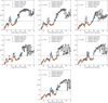 |
Fig. A.1. Compactness parameter ξ2.5of the core-collapse models in this study as a function of their initial helium star mass. The dotted line at ξ2.5 = 0.35 separates most models that might explode (below the line) or implode (above the line). Orange points indicate models that are predicted to explode according to the explodability of the Ertl et al. (2016) and Müller et al. (2016) tests (using their ‘standard’ parameters), blue points are models that are predicted to explode according the Müller et al. (2016) test but not the Ertl et al. (2016) test, green points are models that is predicted to explode according to the Ertl et al. (2016) test but not the Müller et al. (2016) test, and grey points are models that would not successfully explode according to both tests. |
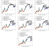 |
Fig. A.2. Compactness parameter ξ2.5of the core-collapse models in this study as a function of their initial helium star mass. The dotted line at ξ2.5 = 0.35 separates most models that might explode (below the line) or implode (above the line). Orange points indicate models that are predicted to explode according to the explodability of the Ertl et al. (2016) and Müller et al. (2016) tests (using their ‘standard’ parameters), blue points are models that are predicted to explode according the Müller et al. (2016) test but not the Ertl et al. (2016) test, green points are models that is predicted to explode according to the Ertl et al. (2016) test but not the Müller et al. (2016) test, and grey points are models that would not successfully explode according to both tests. |
 |
Fig. A.3. Summary of the distribution and relationships between a selection of stellar parameters from our simulations and parameters resulting from the analysis of core-collapse models with Mandel & Müller (2020) model. |
Appendix B: Effect of input parameter variation in the explosion model
In this section we describe the effect of varying the binding energy and the parameters that go into the Müller et al. (2016) and Mandel & Müller (2020) explosion models.
In the main text, we calculate the outcome of the explosion models using a set of parameters given by αout = 0.4, αturb = 1.18, βexpl = 4, ζ = 0.75 and τ1.5 = 1.2. The binding energy that is input into the model is calculated as the sum of the (negative) gravitational energy and the (positive) thermal energy at core collapse. The effect of kinetic energy is neglected (but the kinetic energy is small compared to the other two components), and rotation is not included.
In Sect. B.1 we show the effect of artificially increasing the binding energy of the core-collapse models, and in Sect. B.2 we briefly describe the effect of varying the model parameters.
B.1. Effects of binding energy variation on supernova explosions
To measure the effect of the binding energy of a stellar model at core collapse in the outcome of the Müller et al. (2016) and Mandel & Müller (2020) explosion models, we compare the outcome of our fiducial set of parameters (Fiducial Set) with the outcome that results from calculating the explosion properties using the same set of parameters, but using the approximation of Ebind = −3GM2/5R as a proxy for the binding energy (Set B). This approximation effectively decreases the absolute value of the binding energy outside of the iron core.
As shown in Fig. B.1, the explosion energies are reduced to lower values in Set B, with values that are more in line with the results of Müller et al. (2016). These models have a lower E/M ratio, ranging from about 0.2 to 4 × 1050 erg/ M⊙, with most models having a value of around 2.
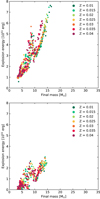 |
Fig. B.1. Explosion energy as a function of final mass from our Fiducial Set (top), and from Set B, calculated with the Müller et al. (2016) model. |
The distribution of NS masses is not heavily affected, although a few models with initial masses in the range 4–10 M⊙ are predicted to produce NSs of more than 1.5 M⊙, while they produce NSs with masses lower than 1.4 M⊙ in the Fiducial Set. However, fewer models result in successful explosions. In most cases, the models that result in successful explosions in the Fiducial Set, but do not produce explosions in Set B, are expected to produce explosions according to the Ertl et al. (2016) criterion. This implies that the resulting distribution of BH masses and the number of BHs per SN are impacted.
When the effect of fallback is included in the calculations, as shown in Fig. B.2, many models that produce NSs in the Fiducial Set produce low-energy explosions that leave behind mass gap BHs instead. In general, explosion energies are lower in Set B than in the Fiducial Set. In the latter case, fallback SNe from models with initial masses higher than about 15 M⊙ produce explosions with energies ranging from 6 × 1051 erg, but can reach energies of up to a few times 1052 erg (not shown in Fig B.2). However, as shown in Sect. 4, they are statistically rare and could be representative of rare, very luminous transients. However, fallback SNe in this regime in Set B produce explosions that are only a few times more energetic than typical SNe, and in many cases in the lower-mass regime such explosions are considerably less energetic than typical SNe.
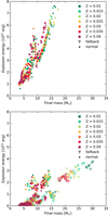 |
Fig. B.2. Explosion energy as a function of final mass from our fiducial set (top) and from set B (bottom), calculated with the Mandel & Müller (2020) model. Circles in the figures correspond to normal SNe, whereas triangles correspond to fallback SNe. |
The initial masses of most of the fallback SNe progenitors in the fiducial set range from about 35 and up to 70 M⊙, whereas in Set B, the models of all masses result in fallback SNe. This has a very large effect on the expected BH and NS mass distributions. In contrast to the Fiducial Set (see Figs. 9 and 10) in Set B we expect most of the NSs resulting from a population of stripped-envelope stars to be around the more massive peak of the NS mass distribution, and most BHs produced are expected to be mass gap objects with masses of about 3 M⊙. In particular, many fallback SNe from models with initial mass lower than 15 M⊙ produce low-energy explosions, have low nickel masses, and no kicks.
Nickel masses in Set B are lower than in the Fiducial Set, regardless of whether we include the effect of fallback or not. Kick velocities in Set B tend to be lower in Set B, and in particular, some models with low explosion energy are also predicted to have 0 kick velocity.
However, regardless of the choice of model, the resulting remnant mass distributions, shown in Fig. B.3, are similar to each other and very different from the typically assumed relations, such as the often used relationships of Fryer et al. (2012). This demonstrates the importance of including detailed, physically motivated explodability prescriptions in population synthesis studies.
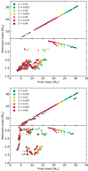 |
Fig. B.3. Remnant masses as a function of final mass from our Fiducial Set (top) and from Set B, calculated with the Müller et al. (2016) model. |
B.2. Effects of parameter variation on supernova explosions
The outcomes of the Müller et al. (2016) and Mandel & Müller (2020) explosion models depend somewhat sensitively on the choice of input parameters. However, many trends and correlations persist in the explosion outcome regardless of the parameter choices.
In this section we describe general trends observed when varying the explosion parameters in both models. In addition to the output of the fiducial set and set B, we calculated several sets of models, varying each parameter independently and keeping all the others fixed, with the same base values as those used by Müller et al. (2016).
Variations in αout result in a significant variation in the number of models that produce successful explosions. We changed the value of αout from 0.3 to 0.7 in steps of 0.1, and found that lower values result in fewer explosions, removing explosions that come from models with low ξ2.5 (below the 0.35 threshold shown in Fig. 5), ant that have low energy compared to the rest of the population. Similarly, explosions with low nickel mass and low kicks are similarly removed when increasing the value of αout. The resulting explosion energies have lower energies than models of similar mass in the Fiducial Set, and a few NSs are formed that are more massive than expected from the correlation between ξ2.5 and the NS mass.
We varied the value of ζ from 0.5 to 0.9 in steps of 0.1. We found that as ζ increases, the initial mass threshold between models that produce successful explosions and those that produce BHs increases. These explosions have a distribution of E/M similar to that of the rest of the explosions with the same given set of parameters and, therefore, are increasingly more energetic. Similarly, such explosions have a higher nickel mass and kick velocity. We varied the value of αturb from 1.14 to 1.22 in steps of 0.02, and of τ1.5 from 1.2 to 1.5 in steps of 0.1, and found no significant differences in the result of our calculations. Therefore, the set of parameters selected as our fiducial set was calibrated by varying αout and ζ to produce a better agreement with the explodability landscape predicted by the Ertl et al. (2016) criterion, resulting in the landscape shown in Fig. A.1.
All Tables
All Figures
|
Fig. 1. Final mass (at core collapse) as a function of initial mass for helium star models of different metallicities. The dots on each line indicate, for each metallicity, the initial helium star mass at which the transition between WN- and WC-type mass loss is observed to occur in the models. The rhombi indicate the value of the minimum luminosity WN-type models obtained from Eq. (8), and using the mass-luminosity relation of Langer (1989). Helium stars below this limit do not have optically thick WR winds and have overestimated mass-loss rates. |
| In the text | |
|
Fig. 2. Final mass of helium in the envelope, as calculated by Eq. (10), shown in solid lines as a function of the initial mass of helium stars of different metallicities. The final total mass of the helium-rich envelope is shown in dashed lines for comparison. The dots on each line indicate, for each metallicity, the initial helium star mass at which the transition between WN- and WC-type mass loss is observed to occur in the models. The rhombi indicate the value of the minimum initial mass above which helium stars are observable as WN-type stars, obtained via Eq. (8). Helium stars below this limit do not have optically thick WR winds and have overestimated mass-loss rates. |
| In the text | |
|
Fig. 3. Surface mass fractions of 4He, 12C, 14N, and 16O of our helium star models at core collapse, as a function of initial mass, for different metallicities. The dots on each line indicate, for each metallicity, the initial helium star mass at which the transition between WN- and WC-type mass loss is observed to occur in the models. |
| In the text | |
|
Fig. 4. Properties of the carbon-oxygen core at the end of helium burning. Top: carbon-oxygen core mass at the end of helium burning, as a function of initial helium star mass. Bottom: central carbon abundance at the end of helium burning, as a function of carbon-oxygen core mass. Thin lines represent models where core carbon burning occurs convectively, whereas thick lines represent models where carbon burning occurs radiatively. The dots on each line indicate, for each metallicity, the initial helium star mass at which the transition between WN- and WC-type mass loss is observed to occur in the models. The rhombi indicate the value of the minimum initial mass above which helium stars are observable as WN-type stars, obtained via Eq. (8). Helium stars below this limit do not have optically thick WR winds and have overestimated mass-loss rates. |
| In the text | |
|
Fig. 5. Compactness parameter as a function of initial mass (top) and final mass (bottom) for helium star models of different metallicities. Circles represent models with final surface abundances that correspond to Type Ib SN progenitors, whereas crosses represent models with surface abundances that correspond to Type Ic SN progenitors. The dashed horizontal line at ξ2.5 = 0.35 divides the majority of exploding models from those that produce BHs. |
| In the text | |
|
Fig. 6. Summary of key parameters obtained from the core-collapse models of helium stars through the explosion model of Müller et al. (2016), as a function of the initial mass (left) and the final mass (right). We include the NS gravitational mass obtained for core-collapse models that successfully explode, the BH mass for models that directly collapse (which corresponds to their final mass), the explosion energy, and the nickel mass. The dashed black lines indicate the division between Type Ib and Type Ic progenitors, and the hashed region corresponds to areas that our model grid does not cover. The horizontal dashed line corresponds to the minimum mass above which models reach core collapse as a WC- or WO-type star, and models to the right of this line are therefore expected to be Type Ic SN progenitors. |
| In the text | |
|
Fig. 7. Same as Fig. 6, but using the explosion model of Mandel & Müller (2020), which includes the effect of fallback. |
| In the text | |
|
Fig. 8. Ratio of explosion energy to ejecta mass inferred using the Mandel & Müller (2020) model as a function of the final mass. The horizontal line at 5 × 1050 erg/M⊙ shows the value of E/M used in Dessart et al. (2020) to produce light curves of Type I SNe. |
| In the text | |
|
Fig. 9. Properties of NS gravitational mass distribution in different metallicities. Top: distribution of NS gravitational masses that result from analysing our core-collapse models with the Mandel & Müller (2020) model, weighted by the IMF from Salpeter (1955), compared to the observed distribution inferred by Antoniadis et al. (2016). The average values of the distributions are represented by vertical lines at the top of the figure. The lowest-mass NSs correspond to progenitors outside of our model grid, and their resulting mass has been assumed to be between 1.22 and 1.3 M⊙. Bottom: Mean value (solid lines) and standard deviation (hatched, shaded regions) of the total distributions and the distributions separated by SN type. The mean value (dashed black line) and the standard deviation (grey line) of the first NS mass peak of the observed distribution of Antoniadis et al. (2016) is shown for comparison. |
| In the text | |
|
Fig. 10. Distribution of BH masses at different metallicities, which results from the analysis of our model with the Mandel & Müller (2020) model, weighted by the IMF from Salpeter (1955). |
| In the text | |
|
Fig. 11. Cumulative distribution functions of ejecta masses, explosion energies, nickel masses, and kick velocities, separated for the full sample of models and separated between Type Ib and Ic SNe that result from analysing our core-collapse models with the Mandel & Müller (2020) model, weighted by the IMF from Salpeter (1955). Different colour lines represent different metallicities. The observed distributions of ejecta masses, explosion energies and nickel masses are drawn from Taddia et al. (2018) for Type Ib, IIb (grouped with Type Ib), and Ic SNe, and additionally from Barbarino et al. (2021) for a larger sample of Type Ic SNe. The average values of each distribution are indicated with vertical lines at the top of each panel. |
| In the text | |
|
Fig. 12. Cumulative distribution of ejecta masses for Type Ib SNe (top) and for all stripped-envelope SNe (bottom) that result from our models, but corrected for the strong variation in wind between WR stars and low-mass helium stars. Here, ejecta masses for stars with initial mass above the minimum mass of WN-type stars are drawn from our model results, and for the rest we assume no mass loss, but the same NS mass as predicted from its original model. |
| In the text | |
|
Fig. 13. Mean values (lines) and standard deviation (shaded region) of the ejecta masses, explosion energies, nickel masses and kick velocities of model populations, obtained by analysing our core-collapse models with the Mandel & Müller (2020) model, weighted by the IMF from Salpeter (1955). These values are shown for the total population of stripped-envelope stars (orange), as well as separated into Type Ib (violet) and Type Ic SNe (blue). For comparison, the mean values and standard deviations of the ejecta masses, the explosion energies, and the nickel masses inferred from the samples of Taddia et al. (2018) and Barbarino et al. (2021) are shown on the right. |
| In the text | |
|
Fig. 14. Number ratios of different quantities as a function of metallicity, as obtained from our model population. Top: number ratio of Type Ib SNe to Type Ic SNe, ⟨NIc/NIb⟩, compared to the observed ratio of Type Ib SNe to Type Ic SNe ⟨NIc/NIb⟩obs and of Type Ib SNe plus Type IIb to Type Ic SNe ⟨NIc/(NIb + NIIb)⟩obs in the local Universe, inferred from the relative rates of Shivvers et al. (2017). Bottom: Number ratio of BHs to SN explosions ⟨NBH/NSN⟩ and number ratio of Type Ib SNe with WR progenitors to Type Ib SNe with transparent-wind helium star progenitors ⟨NIb from WR/NIb from TWHS⟩. |
| In the text | |
|
Fig. A.1. Compactness parameter ξ2.5of the core-collapse models in this study as a function of their initial helium star mass. The dotted line at ξ2.5 = 0.35 separates most models that might explode (below the line) or implode (above the line). Orange points indicate models that are predicted to explode according to the explodability of the Ertl et al. (2016) and Müller et al. (2016) tests (using their ‘standard’ parameters), blue points are models that are predicted to explode according the Müller et al. (2016) test but not the Ertl et al. (2016) test, green points are models that is predicted to explode according to the Ertl et al. (2016) test but not the Müller et al. (2016) test, and grey points are models that would not successfully explode according to both tests. |
| In the text | |
|
Fig. A.2. Compactness parameter ξ2.5of the core-collapse models in this study as a function of their initial helium star mass. The dotted line at ξ2.5 = 0.35 separates most models that might explode (below the line) or implode (above the line). Orange points indicate models that are predicted to explode according to the explodability of the Ertl et al. (2016) and Müller et al. (2016) tests (using their ‘standard’ parameters), blue points are models that are predicted to explode according the Müller et al. (2016) test but not the Ertl et al. (2016) test, green points are models that is predicted to explode according to the Ertl et al. (2016) test but not the Müller et al. (2016) test, and grey points are models that would not successfully explode according to both tests. |
| In the text | |
|
Fig. A.3. Summary of the distribution and relationships between a selection of stellar parameters from our simulations and parameters resulting from the analysis of core-collapse models with Mandel & Müller (2020) model. |
| In the text | |
|
Fig. B.1. Explosion energy as a function of final mass from our Fiducial Set (top), and from Set B, calculated with the Müller et al. (2016) model. |
| In the text | |
|
Fig. B.2. Explosion energy as a function of final mass from our fiducial set (top) and from set B (bottom), calculated with the Mandel & Müller (2020) model. Circles in the figures correspond to normal SNe, whereas triangles correspond to fallback SNe. |
| In the text | |
|
Fig. B.3. Remnant masses as a function of final mass from our Fiducial Set (top) and from Set B, calculated with the Müller et al. (2016) model. |
| In the text | |
Current usage metrics show cumulative count of Article Views (full-text article views including HTML views, PDF and ePub downloads, according to the available data) and Abstracts Views on Vision4Press platform.
Data correspond to usage on the plateform after 2015. The current usage metrics is available 48-96 hours after online publication and is updated daily on week days.
Initial download of the metrics may take a while.