| Issue |
A&A
Volume 659, March 2022
|
|
|---|---|---|
| Article Number | A172 | |
| Number of page(s) | 12 | |
| Section | Extragalactic astronomy | |
| DOI | https://doi.org/10.1051/0004-6361/202142650 | |
| Published online | 23 March 2022 | |
The variability and soft X-ray excess properties of narrow-line Seyfert 1 galaxies: The Swift view
1
School of Physical Science and Technology, Kunming University, Kunming 650214, PR China
e-mail: This email address is being protected from spambots. You need JavaScript enabled to view it.
2
School of Astronomy and Space Science, Nanjing University, Nanjing, Jiangsu 210093, PR China
e-mail: This email address is being protected from spambots. You need JavaScript enabled to view it.
3
Key Laboratory of Modern Astronomy and Astrophysics (Nanjing University), Ministry of Education, Nanjing 210093, PR China
4
Yunnan Observatories, Chinese Academy of Sciences, Kunming 650216, PR China
5
Institute of Astronomy and Astrophysics, Anqing Normal University, Anqing 246133, PR China
6
School of Electrical and Information Technology, Yunnan Minzu University, Kunming, 650091 Yunnan, PR China
7
School of Physics and Electronic Engineering, Jiangsu Second Normal University, Nanjing, Jiangsu 211200, PR China
8
College of Physics and Electronic Engineering, Qujing Normal University, Qujing 655011, PR China
Received:
12
November
2021
Accepted:
27
December
2021
Abstract
We present here a systematic study on the mechanism of the long/short timescale variability and the origin of soft X-ray excess for narrow-line Seyfert 1 galaxies (NLSy1s) based on the multi-epoch multi-band observations of the Swift telescope. The main results are as follows: (1) The ensemble structure functions of radio-quiet NLSy1s in the optical, ultraviolet, and X-ray bands all show a unique double ‘S’ structure. The structural feature reveals that the long and short timescale variability of radio-quiet NLSy1s could be generated by the accretion fluctuation propagation mechanism and the X-ray reprocessing mechanism, respectively, which together cause the complex random light variability. (2) Radio-quiet NLSy1s exhibit significant soft X-ray excess features in their X-ray spectra, but the relative strength of the soft X-ray excess (R) and the power-law spectral index (Γ) do not show a significant positive correlation, unlike what is seen in broad-line Seyfert 1 galaxies (BLSy1s), suggesting that NLSy1s and BLSy1 have different soft X-ray excess mechanisms. After combining the correlation analysis results of model parameters for individual sources at different flux states with the findings in previous work based on XMM-Newton and Suzaku data, we propose that the origin of the soft X-ray excess of NLSy1s prefers the relativistically smeared reflection scenario.
Key words: galaxies: active / galaxies: Seyfert / X-rays: galaxies
© ESO 2022
1. Introduction
In the hot and energetic universe, active galactic nuclei (AGNs) are the most energetic non-catastrophic objects. It is believed that their energies come from the supermassive black holes (SMBHs) in the centre of the galaxy accreting the surrounding matter. The radiation from AGNs spans the entire electromagnetic band, and their complex broadband energy spectrum, random variability, and extreme physical environment make them fascinating objects (see e.g. Padovani et al. 2017). Based on their optical emission lines, AGNs are classified into type-I AGNs and type-II AGNs. The optical emission lines of type-I AGNs have broad and narrow components, while type-II AGNs have only narrow emission lines. The observational differences between type-I and type-II AGNs are successfully explained in the AGN unification model that considers the different types of AGNs to be due to the different observation angles relative to the torus (e.g. Urry & Padovani 1995). Based on the full width at half maximum (FWHM) of the Hβ emission line, type-I AGNs are further divided into broad-line Seyfert 1 galaxies (BLSy1s) and narrow-line Seyfert 1 galaxies (NLSy1s). When the FWHM of the Hβ emission line of the source is less than or greater than 2000 km s−1, the source is classified as an NLSy1 or a BLSy1, respectively (e.g. Goodrich 1989; Rakshit et al. 2017). Compared with BLSy1s, NLSy1s have a strong Fe II emission line and a weak [O III] forbidden line. The FWHM of the Hβ emission line is usually associated with the size of the broad-line region, and the narrower Hβ emission line of NLSy1s implies that they have a small black hole mass. NLSy1s are often found to be accreting at a significant fraction of their Eddington limit. Together with the lower black hole mass, these pieces of information suggest that NLSy1s could be a younger population of AGNs. If this is indeed the case, the study of NLSy1s can lead to important clues on the growth and evolution of SMBHs and black hole physics in an extreme accretion environment (see e.g. Gallo 2018).
Random variability is one of the most special observational characteristics of AGNs. It occurs on different timescales, of minutes, hours, and days, and has been observed in overall accessible waves. In recent years, several phenomenological or physical variability models have been proposed to explain the variability of AGNs at different timescales and different bands, such as the accretion fluctuation propagation model (Lyubarskii 1997), accretion disk instability (Kawaguchi et al. 1998), micro-lensing (Hawkins & Taylor 1997), damped random walk (DRW; Kelly et al. 2009), and X-ray reprocessing (Nandra & George 1994). However, a unified physical picture for the origins of the random variability of AGNs in different timescales and different bands has not been obtained. For NLSy1s, which occupy extreme physical parameters, most of the current research is dedicated to individual sources with extremely significant and special variability, such as Mrk 335, I Zw 1, and PG 1148+273 (see e.g. Wilkins & Gallo 2015; Ding et al. 2021; Wilkins et al. 2021). These studies have successfully revealed that the corona of NLSy1s is highly dynamic and that the structure of the corona undergoes significant changes in a short time (such as a few weeks to several years), resulting in extreme multi-band variation and even X-ray-weak special characteristics. However, the research on the multi-band variability for an NLSy1 sample is limited. In the optical/UV band, Ai et al. (2010), and subsequently Ai et al. (2013), first studied the ensemble structure function (SF) of optical/UV variability for SDSS Strip 82 region sample sources (55 NLSy1s and 108 BLSy1s) with multi-epoch photometric data. They found that NLSy1s have systematically smaller variability than BLSy1s; the amplitude of variability increases with the width of Hβ and the strength of [O III] lines but decreases with the strength of Fe II emission. Using the data of the Catalina real-time transient survey, which span 5−9 years, Rakshit & Stalin (2017) studied the optical/UV variability characteristics of the largest AGN sample to date (5510 NLSy1s and 5510 BLSy1s). Their results further support the findings of Ai et al. (2010, 2013). Compared with the sample research on the optical/UV variability of NLSy1s, the sample research on the X-ray variability of NLSy1s is scarcer.
The emission of type-I AGNs is usually not, or only slightly, absorbed (NH ≤ 1022 cm−2), which allows us to observe the intrinsic X-ray spectrum of the innermost region of such sources. The intrinsic X-ray radiation of AGNs is believed to be the inverse Comptonization of a presumed hot (kT ∼ 100 keV), optically thin (τ ∼ 0.5) corona to the optical/UV photons from the accretion disk (Netzer 2013), and a cutoff power law can usually describe the radiation component with a spectral index of ∼1.8−2 and a cutoff energy of ∼300 keV. In addition, the X-ray spectra of some AGNs show a prominent Compton hump with a peak at ∼30 keV and fluorescence lines, the most important of which is the Fe Kα line at ∼6−7 keV. Below ∼2 keV, many AGNs, especially NLSy1s, show radiation excess compared with the intrinsic power-law emission, called soft X-ray excess. This feature was first discovered by Singh et al. (1985) and Arnaud et al. (1985) using HEAO-I and EXOSAT observations. Subsequently, several theoretical models, such as the partial covering or obstructed model, the relativistically smeared reflection model, and the warm corona model, were proposed to explain this feature. Although there are apparent differences in the physical mechanisms of these models, they can explain the X-ray spectrum with comparative goodness of fit. This makes the physical origin of soft X-ray excess subject to long-standing controversy. To break the degeneracy of these models, some works have used broadband energy spectrum analysis or temporal analysis to study some particular sources. The results show that in different sources, the origin of the soft excess is different and the excess even has ‘hybrid’ characteristics, which implies that the origin of the soft excess is diverse. Systematic sample research will be necessary to reveal the cause and mechanism of the diversity of soft X-ray excess. Gliozzi & Williams (2020) compared the features of the soft X-ray excess of 30 NLSy1s and 59 BLSy1s based on XMM-Newton data. Their results confirmed the previous finding that NLSy1s have a stronger soft X-ray excess component than BLSy1s. They also found a positive correlation between the relative strength of the soft X-ray excess and the primary X-ray spectral index and no correlation between the relative strength of the soft excess and the primary X-ray luminosity for the total sample. They argued that these results support the warm corona origin model of soft X-ray excess. On the contrary, Waddell & Gallo (2020) compared the features of soft X-ray excess of 22 NLSy1s and 47 BLSy1s based on Suzaku data. They noticed differences in the correlation between the relative strength of the soft X-ray excess and the primary X-ray spectral index for NLSy1s and BLSy1s. The two parameters have a positive correlation only in BLSy1s. Furthermore, they found a significant positive correlation between the relative strength of the soft excess and that of hard excess for NLSy1s, suggesting that the origin of the soft X-ray excess of NLSy1s could be explained by the relativistically smeared reflection model.
The Swift space telescope is a NASA space observatory designed to detect gamma-ray bursts (GRBs). It is equipped with three advanced detection instruments: the Burst Alert Telescope (BAT), the X-Ray Telescope (XRT), and the Ultraviolet/Optical Telescope (UVOT). Since the launch of Swift on 20 November 2004, a large amount of multi-band archive data has been accumulated (though not for GRBs). These data provide an excellent opportunity to study the variability and soft X-ray excess properties of NLSy1s in a systematic sample. This paper performs a systematic analysis of the long and short timescale variability and soft X-ray excess properties on an NLSy1 sample based on the Swift data. Thanks to the multi-epoch simultaneous optical/UV and X-ray data provided by the Swift-XRT and Swift-UVOT, we can compare the characteristics of optical/UV and X-ray variability and study the average properties of the soft X-ray excess of the sample or the variation in the soft X-ray excess for individual sources at different flux states, which is difficult to achieve based on XMM-Newton or Suzaku data. The paper is organized as follows. Section 2 describes the sample and data. The variability analyses are shown in Sect. 3. Section 4 presents the X-ray spectral analyses. A detailed discussion of the mechanisms of long/short timescale variability, the properties of X-ray spectra, and the origin of soft X-ray excess is presented in Sect. 5. In Sect. 6 we summarize the main results of this work. The cosmological parameters of H0 = 70 km s−1 Mpc−1, Ωm = 0.3, and ΩΛ = 0.7 are adopted in this work.
2. Sample and data
In order to construct the largest sample of NLSy1s with multi-epoch Swift observations, we cross-matched the present largest sample of NLSy1s compiled by Rakshit et al. (2017) based on the SDSS DR12 with the Swift Master Catalog. Rakshit et al. (2017) performed a spectroscopic reanalysis of 68 859 SDSS DR12 sources classified as ‘QSOs’ using an automatic SDSS spectroscopic pipeline (Richards et al. 2002). The FWHM of Hβ broad emission line < 2200 km s−1 was used as a criterion to identify NLSy1s, and finally 11 101 NLSy1s were identified. We searched the Swift Master Catalog for all observations of these 11 101 NLSy1s with an offset angle of less than 6′ from Swift launch until 1 January 2020. Finally, 699 sources (3482 Swift observations in total) were retrieved. To ensure that samples can perform reliable photometry and time-varying analyses, we require that for each source: (1) there be at least ten Swift-XRT observations with an exposure time of not less than 0.5 ks; and (2) there be at least ten Swift-UVOT observations with an exposure time of not less than 0.5 ks.
Forty-one sources (1291 observations) satisfy the above conditions. We further performed preliminary photometry on the 1291 Swift-XRT observations to obtain their net counts (NCs). The Swift-XRT data of these observations are processed by the task XRTPIPELINE (v0.13.4). The calibration files (CALDB v20180710) and the standard filtering and screening criteria are used in this process. We used the XSELECT tool to extract source NCs. A circular region with a radius of 47″ centred at the object was used as the extracted area of the source, while a source-free annular region with a radius of 70″ slightly away from the object is chosen as the extracted area of the background. To further ensure that the final sample can perform a reliable multi-epoch spectral analysis, it is required that the number of Swift-XRT observations with NC > 35 be not less than ten for each source. Finally, 15 of the 41 sources satisfy this condition, which constitutes the final sample for the analyses in this paper.
The redshift versus 5100 Å luminosity distribution of the parent and final samples is presented in Fig. 1 (left panel). The final sample sources are mainly concentrated in the low-redshift (z < 0.2) region and have relatively high 5100 Å luminosity within a comparable redshift. The black hole mass versus Eddington ratio distribution of the parent and final samples is also shown in Fig. 1 (right panel), where the black hole mass and Eddington ratio parameters are calculated using the method in Sect. 4.6 of Rakshit et al. (2017). There is no significant difference in the distributions of black hole mass and Eddington ratio between the final sample and the parent sample (the Kolmogorov–Smirnov (K-S) test values are 0.323 and 0.425, respectively). The basic information of the 15 sources is listed in Table 1.
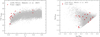 |
Fig. 1. Distributions of the redshift vs. 5100 Å luminosity (left panel) and the black hole mass vs. Eddington ratio (right panel) for the parent and final samples. |
Basic information and the parameter fitting results of the phenomenological model under average state for the 15 NLSy1s.
3. Variability analyses
This section investigates the properties of the long and short timescale variability of the 15 NLSy1s. The energy-dependent characteristic of the variability of each source under the long timescale is first investigated using excess variance spectra (Sect. 3.1). Then, the ensemble SFs of the sample in the optical, UV and X-ray bands are calculated to probe the general temporal properties of NLSy1s (Sect. 3.2).
3.1. Excess variance spectra
Excess variance spectrum, also referred to as fractional variability (Fvar) or root mean square (rms) spectrum, is a tool commonly used to quantify spectral variability (see e.g. Parker et al. 2020). This tool can resolve the energy-dependent features of variability intensity and then distinguish different variable components in the spectrum. Based on the Swift-XRT and Swift-UVOT data, we calculated broadband excess variance spectra for the 15 NLSy1s. Firstly, we performed photometry for the Swift-XRT and Swift-UVOT data of each source to obtain the light curves in the X-ray, three optical (V, B, U), and three UV (W1, M2, W2) bands. For the Swift-XRT data, we used the ‘Swift-XRT products’ generator (Evans et al. 2009) provided by the UK Swift Science Data Centre at the University of Leicester to generate finely processed X-ray light curves. For the Swift-UVOT data, the specific process of photometry is as follows. We summed multiple images in the same filter with the task UVOTIMSUM and then performed aperture photometry with the UVOTSOURCE task for each observation. Source counts are extracted from a circle with a 5″ radius centred on the object, while background counts are extracted from a circle with a 20″ radius located in a source-free region close to the object. The observed magnitudes from aperture photometry are corrected for Galactic extinction using the reddening coefficient from Schlafly & Finkbeiner (2011) and the reddening law with Rv = 3.1 from Fitzpatrick (1999). The corrected observed magnitudes are further converted into fluxes using the zero-point flux following the recipe in Breeveld et al. (2011). Then, based on the light curves obtained from the Swift-XRT and Swift-UVOT data, using Eqs. (10) and (B.2) in Vaughan et al. (2003), we calculated the fractional variability values and their uncertainties in the optical (V, B, U), UV (W1, M2, W2), and 0.3−10 keV X-ray bands to finally integrate the broadband excess variance spectrum.
Figure 2 shows the broadband excess variance spectra of the 15 sources, with the three special sources (J094857.31+002225.5, J084957.98+510829.0, J145108.76+270926.9) being individually labelled in colour. It can be seen that for most NLSy1s, the variability intensity in the X-ray band is more significant than that in the optical/UV bands. The average fraction variability in the optical, UV, and X-ray bands are ∼10%, 17%, and 40%, respectively. There are two sources (J094857.31+002225.5 and J084957.98+510829.0) with completely different characteristics. They show more significant optical variation, with an average fractional variability of up to 100%, and the variation intensity shows an inverse correlation trend with energy. Such characteristics should be attributed to the fact that the two sources are jet-dominated NLSy1s (i.e. radio-loud NLSy1s; see Table 1, they have high radio emissions), and their optical fluxes mainly come from synchrotron emission of relativistic electrons in the jet. The optical emission is usually located near the peak of the synchrotron radiation, which leads to significant variability. Another special source (J145108.76+270926.9) shows very extreme variability in the X-ray band. Compared with other NLSy1s, J145108.76+270926.9 may have additional variability incentives. It can be seen from Table 1 that J145108.76+270926.9 has the highest Eddington ratio among radio-quiet sources. Such an extreme accretion environment could make that coronal configuration (i.e. the height of corona) is highly variable. Indeed, Ding et al. (2021) conducted an in-depth study on the nature of soft X-ray excess and variability of this source by using the multi-epoch XMM-Newton observation data. The results show that the soft X-ray excess of the source is most likely to be originated by the relativistically smeared reflection scenario. In addition, it is found that the X-ray emission has very significant variability in the long and short timescales, in which the short-time variability is related to the intrinsic variation of the corona, while the long-time variability is related to the change of the distance between the corona and the accretion disk.
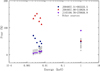 |
Fig. 2. Broadband excess variance spectra of the 15 NLSy1s. Three special sources (J094857.31+002225.5, J084957.98+510829.0, and J145108.76+270926.9) are individually marked in colour. |
3.2. Ensemble structure function
The SF quantifies the variability amplitude (rms of variability) at different time lags, and it has the functionality of the power spectral density (PSD) function (see e.g. Kozłowski 2016). Compared with PSD function, the SF is not sensitive to aliasing problems by discrete or sparse time sampling and can perform an ensemble analysis for a sample (see e.g. Hughes et al. 1992; Middei et al. 2017). The ensemble SF can maximize to extract effective information in the discrete and sparse time-sampling light curves and minimize the impact of some abnormal objects, finally obtaining general (average) variability features of the overall sample. Thus, we use the ensemble SF to analyse the variability features of our sample in the optical, UV and X-ray bands.
When calculating the ensemble SF, we exclude three sources with special variability characteristics in the sample (J094857.31+002225.5, J084957.98+510829.0, and J145108.76+270926.9; see Sect. 3.1). In addition, we combine the light curves of the U, B, and V bands to obtain the ensemble SF of the optical band and combine the light curves of the W1, M2, and W2 bands to obtain the ensemble SF of the UV band. This is because it can be found from Fig. 2 that there is very little difference in the variability in the U, B, and V bands as well as in the W1, M2, and W2 bands. The combined analyses can further overcome the deficiency of sparse sampling.
We used the defining equation of the observed SF shown in Eq. (9) in Kozłowski (2016) to calculate the ensemble SF:
 (1)
(1)
Here y(t) represents the observed fluxes in the optical or UV bands (the net photon counts in the X-ray band) at time t, and NΔt is the number of data pairs in a certain time lag. We correct the observed lag into the rest frame by dividing it by a (1 + z) factor in the calculation. It should be noted that the SF form we adopted does not deduct noise, so we obtain the observed SF rather than the true underlying SF. Therefore, when fitting the observed SF, a full four-parameter expression described by a power exponential form covariance matrix  as shown below needs to be used:
 (2)
(2)
The four parameters in the formula are spectral coefficient β, de-correlation timescale τ, variance at long timescale SF∞, and noise term σn.
Figure 3 shows the ensemble SF calculated in the optical, UV, and X-ray bands, respectively. Interestingly, the ensemble SFs in the optical, UV, and X-ray bands present two substructures: one “S”-shaped structure in the short timescale region and the other in the long timescale region, which implies that there is a transition in the structure of PSD from long timescale to short timescale. Therefore, we use the above four-parameter SF expression to fit the observed data in the short timescale region (the red shadow area in Fig. 3) and the long timescale region (the blue shadow area in Fig. 3), respectively. Here, the fitting ranges for each band are simply determined by visual assessment. The reasonable adjustments of the fitting ranges only make the fitting results change slightly within their uncertainty ranges and not affect the substantive conclusions. In the fittings, the noise term of the SF expression of the long timescale region in the optical and UV bands is determined by the fitting result of short timescale data, while in the X-ray band, the noise term of the SF expression in the short timescale region is determined by the result of the long timescale data. The fitting results are summarized in Table 2. The SF∞ value represents the maximum variability amplitude. It can be noted that the variability amplitude of the X-ray emission is most significant in the short timescale region, while in the long timescale region, the variability amplitude of the optical emission is most significant, showing an overall trend that the ratio of the short timescale maximum variability amplitude to the long timescale maximum variability amplitude decreases with increasing wavelength. The spectral coefficients of the optical/UV SFs are similar in the short and long timescale regions, with the value of ∼2.0 and ∼1.0 in the short and long timescale regions, respectively. The spectral coefficients of the X-ray SFs in the short and long timescale regions are ∼0.9 and ∼1.2, respectively. Such results strongly suggest that there are differences in the mechanisms of long and short timescale variability, and such differences may further contribute to different observed characteristics in the optical/UV and X-ray bands (see Sect. 5.1 for a further discussion).
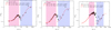 |
Fig. 3. Ensemble SFs in the optical, UV, and X-ray bands, respectively. The solid and dotted red lines are the fitting results of the full four-parameter expression for the data points in the short timescale regime (the red shaded area) and the long timescale regime (the blue shaded area), respectively. |
Fitting results of ensemble SFs in optical, UV, and X-ray bands.
4. X-ray spectra analyses
In this section we investigated the X-ray spectral features of the 15 NLSy1s. Firstly, we performed a fitting of the stacked spectrum of all high-quality X-ray observations based on a phenomenological model to obtain average state model parameters for each source. Then, based on the sample, we conducted a correlation analyses between these model parameters and some physical parameters (e.g. black hole mass). Further, we analysed the variation in the X-ray spectrum of each source to explore the physical origin of the soft X-ray excess.
4.1. Analysis of the X-ray spectra in the average state
Using the Swift-XRT products generator (Evans et al. 2009) from the UK Swift Science Data Centre at the University of Leicester, we extracted X-ray spectra for the high-quality observations (the NCs not less than 15 in both the 0.3−2 keV and 2−10 keV) of the 15 NLSy1s and meanwhile generated a stacked average spectrum for each source. We performed spectral analysis using XSPEC v12.9. All generated spectra are not grouped, and therefore a C-statistics (Cash 1979) are employed to determine the best fit in the fittings. We adopt a phenomenological model wabs*zwabs*((cflux*zpower)+const*(cflux*zbody))) to fit 0.3−10 keV X-ray spectrum, where zbbody approximately represents soft X-ray excess component. the wabs component represents the Galactic absorption, and the Galactic absorption column density of each source is taken from HI4PI Collaboration (2016). The zwabs component is the intrinsic absorption of AGNs. In the above model, the normalization factors of the zbbody and zpower components are fixed to one, and the flux of the zpower component is determined by the cflux. The flux integral range is 0.3−10 keV. The parameters of the cflux of the zbbody component are set to be the same as those of the cflux of the zpower component; the const parameter determines the flux of the zbbody component, and this parameter therefore reflects the relative intensity of the soft X-ray excess to the power-law component. Using the above phenomenological model, we performed fittings on the stacked spectrum of the 15 sources to obtain average state model parameters for each source. The fitting results are presented in Table 1 and Fig. 4.
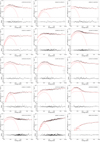 |
Fig. 4. Stacked spectrum fitting results of the 15 NLSy1s. The names of the sources are marked in the upper-left corner of each plane. |
The box plots of the average state model parameters (the relative strength of soft X-ray excess (R), the temperature parameter of zbbody (kT), power-law spectral index (Γ)) of the 13 radio-quiet NLSy1s are shown in Fig. 5. For comparison, the average state model parameters of the two radio-loud NLSy1s are also displayed in these figures with the red pentagram. The distribution of the soft X-ray excess relative strength of the 13 radio-quiet NLSy1s is consistent with the result of Gliozzi & Williams (2020), mainly concentrated in the range of 10−45%. The median of the soft X-ray excess relative strength of the 13 radio-quiet NLSy1s is ∼36.6%, with ∼61% (8/13) of the sources having a soft X-ray excess of more than 30% relative strength. Particularly, SDSS J103438.59+393828.2 has a very high soft excess relative strength of up to 125.5%. The soft excess relative strength of the radio-loud sources is weaker compared to the radio-quiet sources. Four of the radio-quiet NLSy1s have low soft excess relative strength (R < 15%). We examined their X-ray spectra one by one and found that the main reason for two of them is that their X-ray spectra are of poor quality in the low energy. In the remaining two sources (J155909.62+350147.5 and J114116.15+215621.7), the soft X-ray excess component can be clearly seen in their X-ray spectra, but the component indeed is very weak. In short, the observation results strongly confirm that the radio-quiet NLSy1s do generally have significant soft X-ray excess. Still, some individual sources with weaker soft excess features deserve further investigation of the cause in the future. The temperatures of the zbbody component of the sample are concentrated in the range of 0.10 − 0.13 keV, indicating that the soft excess has a constant temperature signature, which is consistent with the previous reports (e.g. Gliozzi & Williams 2020; Waddell & Gallo 2020). Radio-quiet NLSy1s have soft power-law spectral indices, mainly distributed in the range of 2.0 − 2.3, which is consistent with previous reports (e.g. Gliozzi & Williams 2020; Waddell & Gallo 2020). Two radio-loud NLSy1s have a power-law spectral index of ∼1.6, which further indicates the existence of jets.
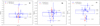 |
Fig. 5. Box plots of the average state model parameters of the 15 NLSy1s. (a) Soft X-ray relative excess intensity. (b) Temperature parameter of the zbbody component. (c) Power-law spectral index. Two radio-loud NLSy1s are marked with the red pentagram. The box represents 25%, 50%, and 75% quantiles of the 13 RQ-NLSy1 data, and the error bar of the box represents the maximum and minimum values of the dataset. |
We further performed a correlation analysis between the average state model parameters obtained above and some physical parameters (black hole mass, Eddington ratio, X-ray variability intensity in the soft and hard bands, and intrinsic X-ray luminosity) on a subsample composed of the 13 radio-quiet NLSy1s in an attempt to find clues to reveal the origin of the soft X-ray excess. The correlation analysis results are presented in the form of a correlogram (see Fig. 6), and the degree of correlation is characterized by the Pearson coefficient. The Pearson correlation coefficient is calculated by a Monte Carlo method similar to that described in Curran (2014), which takes into account the uncertainties on the parameters when conducting the correlation analysis. In Fig. 6 the Pearson correlation coefficients for each parameter pair are given in the top-right grid. The magnitude of the Pearson coefficient can also be reflected by the colour bar on the left of the figure. The correlation between the parameter pairs is graphically represented by an ellipse in the bottom-left grid, with red indicating a positive correlation and blue indicating an inverse correlation. The higher ellipticity means a closer correlation. Significant correlations with confidence levels above 95% are marked with an asterisk.
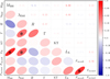 |
Fig. 6. Correlogram of the average state model parameters and other relevant physical parameters (black hole mass, Eddington ratio, intrinsic X-ray luminosity, and X-ray variability intensity in the soft and hard bands). The Pearson correlation coefficients for each parameter pair are given in the top-right grid. The colour bar on the left of the figure reflects the magnitude of the correlation coefficient. The correlation between the parameter pairs is graphically represented by an ellipse in the bottom-left grid, with red indicating a positive correlation and blue indicating an inverse correlation. The higher ellipticity means a closer correlation. Significant correlations with confidence levels above 95% are marked with an asterisk. |
Four significant correlations are presented here. The detailed parameter distribution plots of the four significant correlations and the corresponding linear fitting results are shown in Fig. 7. The significant positive correlation between the X-ray luminosity with the black hole mass and Eddington ratio is a naturally expected result of the accretion system. The Eddington ratio shows a significant positive correlation with the power-law spectral index. This relation has been confirmed in many previous works and is often interpreted as a result of the electron cooling efficiency in the corona being regulated by the accretion rate (e.g. Fabian et al. 2015; Ricci et al. 2018). The best linear fit for this relation is Γ = (0.34 ± 0.10) log λEdd + (2.20 ± 0.06), which is consistent with the result obtained by Waddell & Gallo (2020). There is a significant positive correlation between the variability amplitude of the soft and hard X-ray bands. This correlation is naturally expected for both the relativistically smeared reflection scenario and the warm corona scenario. It, therefore, does not provide a valuable clue to constrain the origin of the soft X-ray excess.
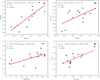 |
Fig. 7. Parameter distribution plots of the four significant correlations and the corresponding linear fitting results. (a) Intrinsic X-ray luminosity vs. black hole mass. (b) Intrinsic X-ray luminosity vs. Eddington ratio. (c) Eddington ratio vs. power-law spectral index. (d) Soft X-ray variability amplitude vs. hard X-ray variability amplitude. The red line is the best linear fit. The linear relation is shown in the upper-left corner of each plane, together with the Pearson correlation coefficient (R) and chance probability (P). |
In addition to the correlations that appear in the correlation analysis described above, it is worth noting that there are two sets of parameters that are not found to be correlated in here.
The first is the correlation result between the soft excess relative strength and the power-law spectral index. Boissay et al. (2016) analysed the features of the soft X-ray excess of 102 Seyfert 1 galaxies from the Swift-BAT 70-month catalogue. They found a significant positive correlation between the soft excess relative strength (R) and the power-law spectral index (Γ) in their sample. This positive correlation favours the warm corona scenario but does not match the theoretical expectation of the relativistically smeared reflection scenario. In the warm corona scenario, the positive correlation could be naturally explained by the increase in the accretion rate enhancing the soft photons from the disk; the increase in the soft photons leads to the enhancement of the soft X-ray fluxes generated by the warm corona and meanwhile improves the cooling efficiency of the hot corona, resulting in a softer photon spectrum. Gliozzi & Williams (2020) analysed and compared the features of the soft X-ray excess of 30 NLSy1s and 59 BLSy1s based on the XMM-Newton data. They found a similar result to Boissay et al. (2016), with a significant positive correlation between R and Γ for the overall sample. However, it is worth noting that when NLSy1s and BLSy1s are considered separately, this positive correlation is only presented in the BLSy1 sample, and the positive correlation found for the overall sample is probably due to the outcome driven by the BLSy1 sample. Unfortunately, Gliozzi & Williams (2020) did not further discuss why this correlation differs in the NLSy1s and BLSy1s. Waddell & Gallo (2020) carried out an in-depth analysis of the X-ray spectra of 22 NLSy1s and 47 BLSy1s using Suzaku observation data. Their results showed that the positive correlation between R and Γ is only presented in the BLSy1 sample but not in the NLSy1s sample. Based on the Swift data, our result further confirms the result of Waddell & Gallo (2020) that there is no positive correlation between R and Γ for the NLSy1s. The difference in the correlation between R and Γ in the NLSy1s and BLSy1s indicates that there could be differences in the origin of the soft X-ray excess between the two types.
The second is the correlation result between the X-ray luminosity and the soft excess relative strength. Gliozzi & Williams (2020) found no significant correlation between the X-ray luminosity and the soft excess relative strength in their sample (30 NLSy1s and 59 BLSy1s). They thought that this result is inconsistent with the theoretical expectation of a negative correlation between the X-ray luminosity and the soft excess relative strength in the absorption or reflection origin models of the soft X-ray excess, so they argued that it is key evidence to exclude the two models. Here, our results also show no significant correlation between the X-ray luminosity and the soft excess relative strength. However, we caution that this result does not serve as evidence to exclude the absorption or reflection origin models of the soft X-ray excess. This is because the current observation results are for the sample as a whole, whereas the inverse correlation between the X-ray luminosity and the soft excess relative strength expected by absorption or reflection models is actually an evolution behaviour of a single source at different flux states. The difference of accretion rate and black hole mass between each source in the sample will make this individual evolution behaviour disappear in the result for the sample as a whole. Therefore, only the correlation result between the X-ray luminosity and the soft excess relative strength for the different epoch (flux state) data of an individual source is meaningful.
4.2. Analysis of the multi-epoch X-ray spectra
Further analyses of the multi-epoch X-ray spectra were carried out for those sources where significant soft X-ray excess (soft excess relative strength higher than 30%) was detected in the average state. We used the phenomenological model adopted in Sect. 4.1 (i.e. wabs*zwabs*((cflux*ZPower)+const*(cflux*zbody))) to fit the X-ray spectrum of each epoch for each source. During the fittings, we noticed that the goodness of fits does not improve significantly when the temperature, kT, in the zbody component is set as a free parameter, and the fitting values of kT between different epochs have only very slight differences. Therefore, this parameter is bound together between different spectra in the final fittings. Finally, there are three free parameters for each spectral fitting: the power-law spectral index (Γ), the relative strength of soft X-ray excess (R), and the power-law flux (F). Based on the fitting results, we performed correlation analysis on the fitting parameters under different flux states for each source. Figure 8 shows the correlation between F and R for each source, and Fig. 9 presents the correlation between F and Γ for each source. The sources displayed in the figure are in descending order according to their soft excess relative strength under the average state. The results of correlation analysis are graphically represented by ellipses. Red indicates positive correlation, and blue represents negative correlation. The higher the ellipticity, the closer the correlation. The Pearson correlation coefficient is marked at the centre of the ellipse. Here the Pearson correlation coefficient is also calculated by a Monte Carlo method similar to that described in Curran (2014), which considers the uncertainties on the parameters when conducting the correlation analysis. The SDSS ID, the soft excess relative strength, the number of observations, and the confidence of the correlation are displayed in the bottom-left corner of each subplot.
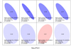 |
Fig. 8. Correlation diagrams of the power-law flux (F) and the relative strength of soft X-ray excess (R) under different flux states for sources where significant soft X-ray excess (soft excess relative strength higher than 30%) was detected in the average state. These sources are displayed in descending order according to their soft excess relative strength under the average state. |
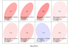 |
Fig. 9. Same as Fig. 8, but for the correlation of the power-law flux (F) and the power-law index (Γ). |
It can be seen from Fig. 8 that except for the source SDSS J123651.17+453904.1, all other sources show a negative correlation between F and R. Especially for the sources with high soft excess relative strength or the sources with more observation times, the negative correlation has high confidence (> 3σ). Conversely, for sources with fewer observations or weaker soft excess strength, the confidence of the negative correlation is low, which is probably only due to the limitation of data quality (weak soft excess strength or fewer observation times). In the reflection model, as the corona approaches the inner region of the black hole, the primary X-ray emission is subjected to an extremely strong light-bending effect, resulting in a weakening of the primary X-ray emission and an enhancement of the reflection component of the disk. As the corona moves away from the inner region of the black hole, the primary X-ray radiation is subjected to a weaker light-bending effect, and the primary X-ray radiation is enhanced while the reflection component is weakened, so an inverse correlation between F and R is expected. This is consistent with our observed trend here. For the correlation between the F and Γ, the result shows that all sources show a positive correlation trend except the source SDSS J123651.17+453904.1. However, except for the source SDSS J103438.59+393828.2, the correlation has a low confidence level for other sources. Therefore, whether the spectral evolution of NLSy1s has a general characteristic of ‘high soft and low hard’ needs to be confirmed by a large sample in the future.
5. Discussion
5.1. Mechanisms of long/short timescale variability
The variability of AGNs presents unpredictable random behaviours, which contain valuable information about the physical process in the innermost region of the black hole. In this work, we calculate the ensemble SFs in the optical, UV, and X-ray bands, respectively, to obtain the general variability features of the radio-quiet NLSy1s. The calculation results show an interesting feature, with the ensemble SFs in the optical, UV, and X-ray bands showing a double ‘S’ structure. The SF value rise with the time lag, reaching a plateau at the timescale of about ten days and then continuing to rise until it flattens out again at about the several-thousand-day timescale. In fact, such a double ‘S’ structure feature has emerged in the previous works on the analysis for the SF of an individual source. Collier & Peterson (2001) analysed the SFs of optical/UV long-term monitoring data for 13 AGNs, and several of the sources (e.g. NGC 5548, MRK 509, MRK 335, and NGC 3783) showed a distinct double ‘S’ structure. Gallo (2018) carried out a detailed SF analysis on the 11-year Swift observation data of MRK 335. They noticed that the SF in the UVW2 (ultraviolet) band exhibits a double ‘S’ structure. They adopted two broken power laws to fit the double ‘S’ structure. The slope of the broken power law in the short-time region (β) is 0.86, and the slope of the broken power law in the long-time region becomes steeper to ≈1.25. This feature is similar to that of the ensemble SF that we obtained in the UV band. Based on the SDSS multi-epoch optical/UV photometric data, Ai et al. (2013) calculated the ensemble SFs of the NLSy1 and BLSy1 in the SDSS strip 82 region, respectively. The results show that the NLSy1 and BLSy1 have similar ensemble SFs in the long timescale region, but BLSy1 have a higher variability amplitude. Towards the short timescale region, the ensemble SF of the BLSy1s shows an additional tentative flattening structure, while the ensemble SF of the NLSy1s continued to decline. Ai et al. suggest that this feature implies that an alternative mechanism, such as X-ray reprocessing, starts to dominate in BLSy1s, but not in NLSy1s, on the short timescales. Different from the result of Ai et al. (2013), our results show that for radio-quiet NLSy1, the additional flattening structure in the short timescale region of the ensemble SF also exists. The reason why Ai et al. (2013) did not find this feature in the NLSy1s is probably due to the limitation of data, as seen in Fig. 9 of Ai et al. (2013), where only three points with large uncertainties are observed in the region of 1−10 days.
The observed double ‘S’ structure in the ensemble SF implies differences in the behaviour and physical mechanism of the long and short timescale variability in the NLSy1s. We further quantify the observed double ‘S’ structure by using two sets of full four-parameter expressions to fit the observed ensemble SF in each band (one set for long timescale data and the other for short timescale data). The fitting results reveal an interesting feature: The SF forms of the short and long timescale regions have a different variation pattern with the band. The SF∞ value increases with the wavelength decrease in the short timescale region, and the SF spectral coefficient decreases with decreasing wavelength. While in the long timescale region, the SF∞ value decreases with the decrease in wavelength, and the spectral coefficient of SF increases with the decrease in wavelength. This feature further indicates that there are differences in the physical mechanism of long and short timescale variability and also implies that there is a potential connection between the physical mechanism of variability in different bands at the same timescale.
In the optical band, the SF spectral index in the long timescale region is β = 0.98 ± 0.41, equivalent to the PSD spectral index of α ∼ 2. This value is consistent with the theoretical expectation of the DRW variability model (see e.g. Kelly et al. 2009; Zu et al. 2013). Based on ground-based optical telescope data, several previous works have found that the DRW variability model can successfully model the long timescale optical variability of AGNs (see e.g. Kelly et al. 2009; MacLeod et al. 2010; Zu et al. 2013). However, in the past ten years, with the acquisition of high-rhythm and high-quality optical variability data from space or ground telescopes, some studies have shown that the short timescale variability behaviour of AGNs deviates from the DRW model, and the observed SF has a steeper spectral index of β ∼ 2 − 3 (Mushotzky et al. 2011; Zu et al. 2013; Caplar et al. 2017; Smith et al. 2018). Our result shows that in the short timescale region, the ensemble SF in the optical band has a steeper spectral index of β = 2.00 ± 0.29, which confirms the previous finding. The ensemble SF in the UV band is similar to that in the optical band on both short and long timescale, suggesting that the original mechanism of UV and optical variability should be consistent (a similar result also found in Collier & Peterson 2001). Nevertheless, it is worth noting that the parameters of the short and long timescale SFs in the UV band are intermediate between those in the optical and X-ray bands and play a transitional role, which is in accord with the fact that the UV radiation region is located between the optical and X-ray emission regions.
In the X-ray band, Middei et al. (2017) calculated the ensemble SF of soft X-ray variability for a sample containing 2864 AGNs in the 3XMM-Newton serendipitous source catalogue by combining the data of ROSAT and XMM-Newton (the observation time baseline is extended to ∼20 years). They found that the ensemble SF value of long timescale X-ray variability increased with the time lag, and no flattening trend of the ensemble SF is observed even up to the ∼20 years timescale. Vagnetti et al. (2016) used the XMM-Newton serendipitous source catalogue DR5 data to explore the ensemble SF of soft X-ray long timescale variability again, and they also obtained a similar result that the ensemble SF value increases with the time lag and does not show a flattening trend even up to an approximately 2000-day timescale. In our work, we calculated the ensemble SF of X-ray variability (0.3−10 keV band) for the radio-quiet NLSy1s. Limited by the data quality in the long timescale (less SF data points and weak variability amplitude), the spectral coefficient (β = 1.16 ± 0.63) and characteristic timescale (τ = 3308.7 ± 1555.7) of the long timescale ensemble SF have significant uncertainty, which hinders the comparison with previous works. Nevertheless, it is worth noting that our result shows that the variability amplitude of short timescale X-ray variability is greater than that of long timescale X-ray variability, and the ensemble SF of X-ray variability does not show a monotonous increase in the entire time lag range as seen in the previous works. Whether this feature is attributable to the peculiar variability property to the NLSy1-type AGNs needs further investigation in future work. In the short timescale, the X-ray variability has a flatter spectral coefficient (β = 0.85 ± 0.34, corresponding α ∼ 1.8) compared to the optical/UV bands. This result is consistent with previous reports (e.g. Simm et al. 2016).
Since the discovery of AGNs, several physical models have been proposed to explain the stochastic variability of AGNs. Although some models have achieved certain success in explaining observations, the complete physical image of the origin of stochastic variability still needs to be integrated and unified. At present, two mechanisms are commonly used to explain the variability of radio-quiet AGNs. One is the accretion fluctuation propagation model, which was first proposed by Lyubarskii (1997). The model considers that the optical/UV variability of AGNs is caused by the propagation of local accretion fluctuation in the whole accretion disk. Since the X-ray emission is generated by the up-scattering of optical/UV photons from the disk by hot electrons in the corona, the optical/UV variability will further lead to the variation in X-ray emission. The variability in the optical/UV band produced by this mechanism usually presents the DRW behaviour. The characteristic timescale is of the order of years, and the intensity of variability is mainly concentrated in the optical band. These features are highly consistent with those observed in the long timescale ensemble SF, suggesting that the long timescale optical/UV variability of NLSy1s is probably due to the accretion fluctuation propagation model, while the long timescale X-ray variability is an associated product due to optical/UV variability. Another major variability mechanism is called the X-ray reprocessing model (Nandra & George 1994). In this model, the optical/UV radiation is produced by the Compton softening process of the irradiated cold accretion disk surface. In this process, the intrinsic short timescale X-ray variability in the corona causes the optical/UV variation in the timescale of the order of days, and the intensity of the X-ray variability is naturally expected to be more significant than that in the optical/UV band. These characteristics are consistent with those observed in the short timescale ensemble SF, suggesting that the short timescale optical/UV variation in NLSy1s is most likely due to the X-ray reprocessing model. Therefore, on the whole, the long and short timescale variability of NLSy1 could be caused by the accretion fluctuation propagation model and the X-ray reprocessing model, respectively, which together drive the complex random variation characteristics of NLSy1.
5.2. Properties of X-ray spectra and the origin of the soft X-ray excess
In this work, we performed the average state analysis and multi-epoch variation analysis on the X-ray spectra of sources with high-quality multi-epoch observations. The results of the average state analysis show that most radio-quiet NLSy1s have strong soft X-ray excess components, with a relative strength ranging from 10% to 45%. The temperature of the blackbody component characterizing the soft X-ray excess has a stable value, ranging from 0.1 to 0.12 keV, and these radio-quiet NLSy1s has a steep hard X-ray spectrum with a spectral index in the range of ∼2.0−2.3. These observational features are consistent with the properties of NLSy1s reported in previous studies (e.g. Gallo 2018; Gliozzi & Williams 2020; Waddell & Gallo 2020). The correlation analysis for the average model parameters of a radio-quiet NLSy1 sample reveals a known significant positive correlation between the Eddington ratio and the power-law spectral index and a significant positive correlation between the variability amplitude of 0.2−2 keV and 2−10 keV. The former is a signature of the accretion rate regulating the coronal electron cooling efficiency, and the latter is the natural expectation of the disk-corona accretion system.
An interesting result is that based on the Swift data, we further confirm the results obtained based on the Suzaku and the XMM-Newton data, that is, different from BLSy1s, there is no positive correlation between R and Γ for NLSy1s (Gliozzi & Williams 2020; Waddell & Gallo 2020). In addition, we note that Waddell & Gallo (2020) found that the intensity of the soft X-ray excess has a significant positive correlation with the intensity of the hard X-ray excess for NLSy1s, but in the BLSy1 sample, the intensity of soft X-ray excess have a very narrow distribution range, which makes that there is no correlation between the soft X-ray excess intensity and the hard X-ray excess intensity for BLSy1s. The differences in the above statistical relations between NLSy1s and BLSy1s strongly suggest that there could be a diversity in the origin of the soft X-ray excess between NLSy1s and BLSy1s. There are two mainstream models for the origin of the soft X-ray excess, the warm corona model and the relativistically smeared reflection model. However, due to the high degeneracy of the two models for spectral fitting, there are great disputes between the two models so far. There are differences between the two models in the theoretical expectation of the correlation between R and Γ and the correlation between the soft X-ray excess intensity and the hard X-ray excess intensity. In the warm corona model, the association of the warm corona with the disk and the hot corona naturally expects a positive correlation between R and Γ; In the relativistically smeared reflection model, the association of the high-energy reflection with the low-energy reflection naturally expects a positive correlation between the soft X-ray excess intensity and the hard X-ray excess intensity. Therefore, the observation results imply that the origin of the soft X-ray excess of NLSy1s is the relativistically smeared reflection model, whereas, in BLSy1s, the warm corona model is favoured. Consistent with the result of Gliozzi & Williams (2020) based on the XMM-Newton data, we did not find any correlation between the intrinsic X-ray luminosity and the soft X-ray excess intensity for the whole NLSy1 sample, but it should be emphasized again that this result cannot be used as evidence to exclude the relativistically smeared reflection model (see explanation in Sect. 4.2). Thanks to the Swift telescope providing multi-epoch observations for a single source, we performed a correlation analysis between the X-ray luminosity and the soft X-ray excess intensity at different flux states for each source with significant soft X-ray excess. The results show that for sources with strong soft X-ray excess intensity or with a large number of observations (i.e. having a high-quality statistical foundation), the X-ray luminosity and the soft X-ray excess intensity show a significant anti-correlation expected by the relativistically smeared reflection model. This result further supports that the origin of the soft X-ray excess of NLSy1s prefers the relativistically smeared reflection model.
6. Conclusion
This paper investigates the characteristics and the origin mechanism of the long/short timescale variability of NLSy1s using multi-epoch multi-band data provided by the Swift telescope. The properties of the soft X-ray excess are also investigated based on a model-independent spectral analysis. Our two main results are as follows.
First, the observed ensemble SFs of radio-quiet NLSy1s exhibit a unique double ‘S’ structure in the optical, UV, and X-ray bands. This structural feature reveals a physical picture of random variability: the long and short timescale variability of NLSy1s is produced by the accretion fluctuation propagation and X-ray reprocessing mechanisms, respectively, which combine to form observed complex random variability.
Second, radio-quiet NLSy1s have significant soft X-ray excess features in their X-ray spectra, but the soft X-ray excess relative strength (R) and the power-law spectral index (Γ) are not found to have a significant positive correlation, unlike what is seen in BLSy1s. Combining the results of model parameter correlation analysis for individual source at different flux states with the findings of previous work based on XMM-Newton and Suzaku data, we propose that the difference in the model parameter correlation between NLSy1s and BLSy1s indicates that the two have different soft X-ray excess mechanisms. For the origin of the soft X-ray excess of NLSy1s, the relativistically smeared reflection scenario is favoured.
Acknowledgments
We sincerely thank the anonymous referee for helpful suggestions. We are grateful for the financial support from the National Natural Science Foundation of China (No. 12103022) and the Special Basic Cooperative Research Programs of Yunnan Provincial Undergraduate Universities’ Association (No. 202101BA070001-043). This work is also supported by the National Key Research and Development Program of China (No. 2017YFA0402703) and by the National Natural Science Foundation of China (No. 11733002, 12121003, 12192220, and 12192222). We also acknowledge the science research grants from the China Manned Space Project with NO. CMS-CSST-2021-A05. Y.Y.T. acknowledges the financial support from the Yunnan Talent Program for Young Top-Notch Talents (YNWR-QNBJ-2020-076). D.R.X. acknowledges the financial support from the Yunnan Province Foundation (2019FB004). This work made use of the Swift data and the data supplied by the UK Swift Science Data Centre at the University of Leicester.
References
- Ai, Y. L., Yuan, W., Zhou, H. Y., et al. 2010, ApJ, 716, L31 [NASA ADS] [CrossRef] [Google Scholar]
- Ai, Y. L., Yuan, W., Zhou, H., et al. 2013, AJ, 145, 90 [Google Scholar]
- Arnaud, K. A., Branduardi-Raymont, G., Culhane, J. L., et al. 1985, MNRAS, 217, 105 [NASA ADS] [CrossRef] [Google Scholar]
- Boissay, R., Ricci, C., & Paltani, S. 2016, A&A, 588, A70 [NASA ADS] [CrossRef] [EDP Sciences] [Google Scholar]
- Breeveld, A. A., Landsman, W., Holland, S. T., et al. 2011, in Gamma Ray Bursts 2010, eds. J. E. McEnery, J. L. Racusin, & N. Gehrels, AIP Conf. Ser., 1358, 373 [Google Scholar]
- Caplar, N., Lilly, S. J., & Trakhtenbrot, B. 2017, ApJ, 834, 111 [NASA ADS] [CrossRef] [Google Scholar]
- Cash, W. 1979, ApJ, 228, 939 [Google Scholar]
- Collier, S., & Peterson, B. M. 2001, ApJ, 555, 775 [NASA ADS] [CrossRef] [Google Scholar]
- Curran, P. A. 2014, ArXiv e-prints [arXiv:1411.3816] [Google Scholar]
- Ding, N., Gu, Q., Tang, Y., et al. 2021, A&A, 650, A183 [NASA ADS] [CrossRef] [EDP Sciences] [Google Scholar]
- Evans, P. A., Beardmore, A. P., Page, K. L., et al. 2009, MNRAS, 397, 1177 [Google Scholar]
- Fabian, A. C., Lohfink, A., Kara, E., et al. 2015, MNRAS, 451, 4375 [Google Scholar]
- Fitzpatrick, E. L. 1999, PASP, 111, 63 [Google Scholar]
- Gallo, L. 2018, Revisiting Narrow-Line Seyfert 1 Galaxies and their Place in the Universe, 34 [Google Scholar]
- Gliozzi, M., & Williams, J. K. 2020, MNRAS, 491, 532 [Google Scholar]
- Goodrich, R. W. 1989, ApJ, 340, 190 [NASA ADS] [CrossRef] [Google Scholar]
- Hawkins, M., & Taylor, A. 1997, ApJ, 482, L5 [CrossRef] [Google Scholar]
- HI4PI Collaboration (Ben Bekhti, N., et al.) 2016, A&A, 594, A116 [NASA ADS] [CrossRef] [EDP Sciences] [Google Scholar]
- Hughes, P. A., Aller, H. D., & Aller, M. F. 1992, ApJ, 396, 469 [NASA ADS] [CrossRef] [Google Scholar]
- Kawaguchi, T., Mineshige, S., Umemura, M., & Turner, E. L. 1998, ApJ, 504, 671 [NASA ADS] [CrossRef] [Google Scholar]
- Kelly, B. C., Bechtold, J., & Siemiginowska, A. 2009, ApJ, 698, 895 [Google Scholar]
- Kozłowski, S. 2016, ApJ, 826, 118 [CrossRef] [Google Scholar]
- Lyubarskii, Y. E. 1997, MNRAS, 292, 679 [Google Scholar]
- MacLeod, C. L., Ivezić, Ž., Kochanek, C. S., et al. 2010, ApJ, 721, 1014 [Google Scholar]
- Middei, R., Vagnetti, F., Bianchi, S., et al. 2017, A&A, 599, A82 [NASA ADS] [CrossRef] [EDP Sciences] [Google Scholar]
- Mushotzky, R. F., Edelson, R., Baumgartner, W., & Gandhi, P. 2011, ApJ, 743, L12 [NASA ADS] [CrossRef] [Google Scholar]
- Nandra, K., & George, I. M. 1994, MNRAS, 267, 974 [NASA ADS] [Google Scholar]
- Netzer, H. 2013, The Physics and Evolution of Active Galactic Nuclei (Cambridge: Cambridge University Press) [Google Scholar]
- Padovani, P., Alexander, D., Assef, R., et al. 2017, A&ARv, 25, 1 [NASA ADS] [CrossRef] [Google Scholar]
- Parker, M., Alston, W., Igo, Z., & Fabian, A. 2020, MNRAS, 492, 1363 [NASA ADS] [CrossRef] [Google Scholar]
- Rakshit, S., & Stalin, C. S. 2017, ApJ, 842, 96 [NASA ADS] [CrossRef] [Google Scholar]
- Rakshit, S., Stalin, C. S., Chand, H., & Zhang, X.-G. 2017, ApJS, 229, 39 [Google Scholar]
- Ricci, C., Ho, L. C., Fabian, A. C., et al. 2018, MNRAS, 480, 1819 [NASA ADS] [CrossRef] [Google Scholar]
- Richards, G. T., Fan, X., Newberg, H. J., et al. 2002, AJ, 123, 2945 [NASA ADS] [CrossRef] [Google Scholar]
- Schlafly, E. F., & Finkbeiner, D. P. 2011, ApJ, 737, 103 [Google Scholar]
- Simm, T., Salvato, M., Saglia, R., et al. 2016, A&A, 585, A129 [NASA ADS] [CrossRef] [EDP Sciences] [Google Scholar]
- Singh, K. P., Garmire, G. P., & Nousek, J. 1985, ApJ, 297, 633 [NASA ADS] [CrossRef] [Google Scholar]
- Smith, K. L., Mushotzky, R. F., Boyd, P. T., et al. 2018, ApJ, 857, 141 [NASA ADS] [CrossRef] [Google Scholar]
- Urry, C. M., & Padovani, P. 1995, PASP, 107, 803 [NASA ADS] [CrossRef] [Google Scholar]
- Vagnetti, F., Middei, R., Antonucci, M., Paolillo, M., & Serafinelli, R. 2016, A&A, 593, A55 [NASA ADS] [CrossRef] [EDP Sciences] [Google Scholar]
- Vaughan, S., Edelson, R., Warwick, R. S., & Uttley, P. 2003, MNRAS, 345, 1271 [Google Scholar]
- Waddell, S. G. H., & Gallo, L. C. 2020, MNRAS, 498, 5207 [NASA ADS] [CrossRef] [Google Scholar]
- Wilkins, D. R., & Gallo, L. C. 2015, MNRAS, 449, 129 [NASA ADS] [CrossRef] [Google Scholar]
- Wilkins, D. R., Gallo, L. C., Costantini, E., Brandt, W. N., & Blandford, R. D. 2021, Nature, 595, 657 [NASA ADS] [CrossRef] [Google Scholar]
- Zu, Y., Kochanek, C. S., Kozłowski, S., & Udalski, A. 2013, ApJ, 765, 106 [NASA ADS] [CrossRef] [Google Scholar]
All Tables
Basic information and the parameter fitting results of the phenomenological model under average state for the 15 NLSy1s.
All Figures
|
Fig. 1. Distributions of the redshift vs. 5100 Å luminosity (left panel) and the black hole mass vs. Eddington ratio (right panel) for the parent and final samples. |
| In the text | |
|
Fig. 2. Broadband excess variance spectra of the 15 NLSy1s. Three special sources (J094857.31+002225.5, J084957.98+510829.0, and J145108.76+270926.9) are individually marked in colour. |
| In the text | |
|
Fig. 3. Ensemble SFs in the optical, UV, and X-ray bands, respectively. The solid and dotted red lines are the fitting results of the full four-parameter expression for the data points in the short timescale regime (the red shaded area) and the long timescale regime (the blue shaded area), respectively. |
| In the text | |
|
Fig. 4. Stacked spectrum fitting results of the 15 NLSy1s. The names of the sources are marked in the upper-left corner of each plane. |
| In the text | |
|
Fig. 5. Box plots of the average state model parameters of the 15 NLSy1s. (a) Soft X-ray relative excess intensity. (b) Temperature parameter of the zbbody component. (c) Power-law spectral index. Two radio-loud NLSy1s are marked with the red pentagram. The box represents 25%, 50%, and 75% quantiles of the 13 RQ-NLSy1 data, and the error bar of the box represents the maximum and minimum values of the dataset. |
| In the text | |
|
Fig. 6. Correlogram of the average state model parameters and other relevant physical parameters (black hole mass, Eddington ratio, intrinsic X-ray luminosity, and X-ray variability intensity in the soft and hard bands). The Pearson correlation coefficients for each parameter pair are given in the top-right grid. The colour bar on the left of the figure reflects the magnitude of the correlation coefficient. The correlation between the parameter pairs is graphically represented by an ellipse in the bottom-left grid, with red indicating a positive correlation and blue indicating an inverse correlation. The higher ellipticity means a closer correlation. Significant correlations with confidence levels above 95% are marked with an asterisk. |
| In the text | |
|
Fig. 7. Parameter distribution plots of the four significant correlations and the corresponding linear fitting results. (a) Intrinsic X-ray luminosity vs. black hole mass. (b) Intrinsic X-ray luminosity vs. Eddington ratio. (c) Eddington ratio vs. power-law spectral index. (d) Soft X-ray variability amplitude vs. hard X-ray variability amplitude. The red line is the best linear fit. The linear relation is shown in the upper-left corner of each plane, together with the Pearson correlation coefficient (R) and chance probability (P). |
| In the text | |
|
Fig. 8. Correlation diagrams of the power-law flux (F) and the relative strength of soft X-ray excess (R) under different flux states for sources where significant soft X-ray excess (soft excess relative strength higher than 30%) was detected in the average state. These sources are displayed in descending order according to their soft excess relative strength under the average state. |
| In the text | |
|
Fig. 9. Same as Fig. 8, but for the correlation of the power-law flux (F) and the power-law index (Γ). |
| In the text | |
Current usage metrics show cumulative count of Article Views (full-text article views including HTML views, PDF and ePub downloads, according to the available data) and Abstracts Views on Vision4Press platform.
Data correspond to usage on the plateform after 2015. The current usage metrics is available 48-96 hours after online publication and is updated daily on week days.
Initial download of the metrics may take a while.