| Issue |
A&A
Volume 658, February 2022
|
|
|---|---|---|
| Article Number | A117 | |
| Number of page(s) | 8 | |
| Section | Stellar atmospheres | |
| DOI | https://doi.org/10.1051/0004-6361/202142372 | |
| Published online | 09 February 2022 | |
MUSE crowded field 3D spectroscopy in NGC 300
II. Quantitative spectroscopy of BA-type supergiants
1
European Southern Observatory (ESO),
Karl-Schwarzschild-Str. 2,
85748
Garching bei München,
Germany
e-mail: Gemma.GonzaleziTora@eso.org
2
Astrophysics Research Institute, Liverpool John Moores University,
146 Brownlow Hill,
Liverpool
L3 5RF,
UK
3
Institut für Astro- und Teilchenphysik, Universität Innsbruck,
Technikerstr. 25/8,
6020
Innsbruck,
Austria
4
Institute for Astrophysics, University of Göttingen,
Friedrich-Hund-Platz 1,
37077
Göttingen,
Germany
5
Leibniz-Institut für Astrophysik (AIP),
An der Sternwarte 16,
14482
Postdam,
Germany
Received:
5
October
2021
Accepted:
17
December
2021
Aims. A quantitative spectral analysis of BA-type supergiants and bright giants in an inner spiral arm region of the nearby spiral galaxy NGC 300 is presented, based on observations with the Multi Unit Spectroscopic Explorer (MUSE) on the European Southern Obsevatory, Very Large Telescope. The flux-weighted gravity–luminosity relationship (FGLR), a stellar spectroscopic distance determination method for galaxies, is extended towards stars at lower luminosities.
Methods. Point spread function fitting 3D spectroscopy was performed with PampelMUSE on the datacube. The 16 stars with the highest signal-to-noise ratios are classified with regard to their spectral type and luminosity class using Galactic templates. They were analysed using hybrid non-local thermodynamic equilibrium model spectra to fit the strongest observed hydrogen, helium, and metal lines in the intermediate-resolution spectra. Supplemented by photometric data, this facilitates fundamental stellar parameters and interstellar reddening which have yet to be determined.
Results. Effective temperatures, surface gravities, reddening E(B−V), bolometric magnitudes and luminosities, as well as radii and masses are presented for the sample stars. The majority of the objects follow the FGLR as established from more luminous BA-type supergiants in NGC 300. An increase in the scatter in the flux-weighted gravity–luminosity plane is observed at these lower luminosities, which is in line with predictions from population synthesis models.
Key words: stars: atmospheres / stars: early-type / stars: fundamental parameters / supergiants / galaxies: distances and redshifts / galaxies: individual: NGC 300
© ESO 2022
1 Introduction
Historic turning points in astronomy were the identification of the true nature of galaxies by resolving their stellar content (Hubble 1929) and the identification of stellar populations (Baade 1944), which facilitated an understanding of galaxy evolution which has yet to be developed. Currently, this can be achieved for galaxies out to distances in the nearest clusters of galaxies using the Hubble Space Telescope or the ground-based 8–10 m telescopes.
Far more challenging is the spectroscopy of individual stars in other galaxies. Early spectroscopic observations with 4 m-class telescopes showed that the visually brightest stars in the Local Group galaxies and beyond are massive blue supergiants of late B and A spectral types (BA-type supergiants), reaching absolute visual magnitudes of MV ≃ − 9.5 (e.g. Humphreys & Davidson 1979; Humphreys & Aaronson 1987). These stars are typically evolved objects crossing the Hertzsprung-Russell diagram (HRD) for the first time towards the red after terminating their main-sequence phase as OB-type stars. They reach their high visual brightness because of the low bolometric corrections at these temperatures, that is MV ≃Mbol.
The potential of the stars for quantitative analyses over larger distances was previously identified, leading to the first determination of atmospheric parameters and chemical abundances of the Galactic prototype A-type supergiant Deneb by Groth (1961) and the brightest BA-type supergiants in the Magellanic Clouds (Przybylski 1968, 1971, 1972; Wolf 1972, 1973), all based on Coudé spectra recorded on photographic plates. However, systematic studies of samples of A-type supergiants in the Milky Way and the Small Magellanic Cloud (SMC) at high spectral resolution were only performed much later (Venn 1995a,b, 1999), based on Coudé and Echelle spectra recorded with CCD detectors. At about the same time, the first quantitative analyses of a few individual BA-type supergiants in galaxies of the Local Group beyond the Magellanic Clouds were undertaken based on Echelle spectra taken with Keck and the European Southern Observatory (ESO) Very Large Telescope (VLT) in M 33, M 31, NGC 6822, and WLM (McCarthy et al. 1995; Venn et al. 2000, 2001, 2003).
A more efficient use of telescope time was promised by multi-slit spectrographs at intermediate spectral resolution by increasing the number of simultaneously observed targets to about 20, for example with the visual and near UV FOcal Reducer and low dispersion Spectrograph (FORS) on the VLT (Appenzeller et al. 1998) or the Low Resolution Imaging Spectrometer (LRIS) on Keck (Oke et al. 1995). BA-type supergiants are bright enough to be observable in galaxies out to the Virgo cluster with 8–10 m telescopes (Kudritzki et al. 1995). Practical limitations, in particular crowding at seeing-limited conditions, restrict quantitative studies to about a 7 Mpc distance, such as in NGC 3621 (Bresolin et al. 2001; Kudritzki et al. 2014) or the maser-host galaxy NGC 4258 (Kudritzki et al. 2013). Studies encompassed nearby metal-poor irregular galaxies such as WLM (Urbaneja et al. 2008), IC1613 (Berger et al. 2018), or NGC 3109 (Hosek et al. 2014). At the focus of investigations stood galactic abundance gradients (e.g. Kudritzki et al. 2008) and the comparison of stellar and nebular abundance indicators (e.g. Urbaneja et al. 2005; Bresolin et al. 2009, 2016). A closely related field was the investigation of the galaxy mass–metallicity relationship (e.g. Lequeux et al. 1979; Tremonti et al. 2004) based on stellar indicators (Kudritzki et al. 2012), which help to overcome uncertainties from employing strong-line-methods for nebular analyses (Kewley & Ellison 2008; Andrews & Martini 2013). In addition, contributions were made to establish a novel spectroscopic distance indicator, the flux-weighted gravity-luminosity relationship (FGLR, Kudritzki et al. 2003, 2008) by concentrating on important calibrators of the extragalactic distance scale such as the Large Magellanic Cloud (LMC, Urbaneja et al. 2017) and M 33 (U et al. 2009).
A particular role for stellar studies in systems of the nearby galaxy groups play those towards the filamentary Sculptor Group (Karachentsev et al. 2003) as they are located close to the Galactic southern pole, that is these are the galaxies affected least by Galactic extinction. In the foreground – at distances shortly below 2 Mpc – are NGC 55 (Castro et al. 2012; Kudritzki et al. 2016)and NGC 300. As a spiral galaxy seen nearly face-on, the latter one has attracted many quantitative investigations using multi-object slit spectroscopy (Bresolin et al. 2002, 2004, 2009; Urbaneja et al. 2003, 2005; Kudritzki et al. 2008)
Innovation on the instrumental side in the form of integral field spectroscopy (IFS) or 3D spectroscopy promises to increase the multiplex further by more than an order of magnitude. This technique allows for a spectrum for each pixel across an image to be obtained simultaneously. It is an extremely powerful and fast tool to perform spectroscopy on extended objects. Groundbreaking in this context is the Multi Unit Spectroscopic Explorer (MUSE, Bacon et al. 2014) on the ESO VLT, which combines a wide field of view with high spatial sampling (1′×1′ field with 0.′′2 sampling). The first surveys of the massive star populations in nearby galaxies have already started with MUSE. Demonstrations were made for dense star clusters in the LMC (Castro et al. 2018, 2021) and SMC (Bodensteiner et al. 2020), and for wider fields in the Sculptor Group galaxies NGC 300 (Roth et al. 2018, henceforth Paper I) and NGC 7793 (Wofford et al. 2020).
The present study aims to provide a detailed analysis of MUSE spectra of BA-type supergiants and bright giants in NGC 300 in one field from Paper I based on synthetic spectra that account for deviations from local thermodynamic equilibrium (LTE). The paper is organised as follows: a brief overview of the observations, the data reduction, and the source extraction is given in Sect. 2. Section 3 gives an overview of the employed models as well as describes the spectral analysis and the resulting atmospheric and fundamental stellar parameters. A discussion of the results, in particular focussing on an extension of the FGLR towards lower luminosities, is presented in Sect. 4. Finally, prospects for future work are discussed in Sect. 5.
2 Observations and data reduction
The spectroscopic data were obtained using MUSE (Bacon et al. 2014), which is located on the Unit Telescope 4 (UT4) Nasmyth focus of the VLT at Paranal Observatory in Chile. The wide field mode (WFM) with 1′×1′ spatial coverage and 0.′′2 sampling was used. The data discussed here were taken prior to the adaptive optics (AO) improvement as implemented via the GALACSI module to the MUSE facility.
Therefore, the pointing observed under the best seeing conditions (FWHM = 0.′′47–0.′′59, measured from the data) was investigated, that is the one that promises the best spatial resolution and highest signal-to-noise ratio (S/N) per extracted spectrum. This corresponds to field (i) of Paper I (see their Fig. 1). The three observations of this field were carriedout on October 30, 2014 and on November 24 and 25, 2014, with an exposure time of 1800 s each at an airmass of 1.03–1.05. The data obtained with the WFM have an intermediate spectral resolving power of R = λ∕Δλ ≈ 1800–3600, a dispersion of 1.25 Å pixel−1, and cover the wavelength range from 4650 to 9300 Å (extended wavelength range).
The initial reduction was achieved with the MUSE pipeline V1.0 (Weilbacher et al. 2020, see Paper I for details). The final data were produced in the form of a datacube, and the spectra of 606 individual sources were extracted using the PampelMUSE software (Kamann et al. 2013).
Out of these 606 extracted sources, 26 were classified as late-B to early-A supergiants or bright giants in Paper I with a minimum S∕N > 7, which was imposed in order for our analysis to provide meaningful results. They are identified in Fig. 1, which shows NGC 300 field (i) in spaxel coordinates. The stars cover deprojected galactocentric distances of 1.4–1.9 kpc when adopting the following NGC 300 galaxy parameters from the HyperLEDA database (Makarov et al. 2014): galaxy centre RA(J2000) = 00:54:53.54/Dec(J2000) = −37:41:04.3, an inclination between the line of sight and the polar axis of the galaxy 48(((fdg)))5, a major axis position angle of 113(((fdg)))2, and a distance of 1.86 Mpc (Rizzi et al. 2006).
The spectroscopic data were complemented by Johnson photometry in the B and V bands obtained with the Wide Field Imager (WFI) at the ESO/MPI 2.2 m telescope on La Silla. These data were previously employed in stellar studies of NGC 300 (Bresolin et al. 2002, 2004). Details of the calibration and reduction of these data were discussed by Pietrzyński et al. (2002).
The observational properties of the 26 stars are summarised in Table 1. The stars were identified by an ID number (adopted from Paper I), the RA and Dec coordinates are given, Johnson V magnitudes and (B−V) colours are stated, the S/N of the extracted spectra are indicated, and comments on individual stars are given, where appropriate.For two stars, no Johnson photometric data are available. Four objects show, in their spectra, emission lines that are characteristic of low-excitation H II regions, such as [N II] and [S II], and very weak [O III]. The stellar hydrogen lines are therefore expected to be contaminated by nebular emission. Moreover, the stars are too cool to excite the nebulae; therefore, it is likely that nearby OB-type stars contribute to the recorded spectra. Finally, four more stars will later turn out to have atmospheric parameters that lie beyond those covered by our model grids. Consequently, only 16 objects fulfilled the criteria for a quantitative analysis, which is discussed in the following.
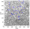 |
Fig. 1 Chart of NGC 300 field (i) with the programme stars marked in red and their ID numbers in blue (according to Paper I). The image is stacked over all recorded wavelengths in the datacube. |
3 Analysis
3.1 Models
We adopt the modelling methodology developed by Przybilla et al. (2006) for the analysis of our final sample of 16 stars. Very briefly, a combination of model atmosphere structures calculated under the assumption of LTE and a detailed non-LTE level population as well as line-formation calculations are employed. The reader is referred to Przybilla et al. (2006) for an extensive discussion of the advantages and drawbacks of this hybrid approach, as well as its applicability limits. To ensure these limits are respected, the analyses are restricted to the brightest late B-type and A-type giant and supergiant stars in the observed sample, which initially corresponds to the 26 stars shown in Table 1. For the reasons already mentioned, we obtain a final sample of 16 stars.
Following previous work on the quantitative analysis of low resolution optical spectra of extragalactic BA-type supergiants (see for example Kudritzki et al. 2008), we initially considered a grid of model atmospheres exploring the parameter space defined by the effective temperature Teff, surface gravity log g, global metallicity ![$\left[Z\right]$](/articles/aa/full_html/2022/02/aa42372-21/aa42372-21-eq1.png) , and microturbulence ξ. The location of the stars in the disk of the galaxy at galactocentric distances between 1.4 and 1.9 kpc, in combination with the NGC 300 metallicity gradient (Kudritzki et al. 2008; Gazak et al. 2015), constrains the metallicity at an average [Z] = −0.2 dex, that is to say slightly lower than solar. To explore the limitations of our models, we used the available grids with both [Z] = 0 dex and [Z] = −0.15 dex and found that the results of the analysis using both [Z] changed by ≲200 K in temperature, and ≲0.05 dex in log gravity, so both results agree within the error limits. Furthermore, following the results obtained in the high resolution work by Przybilla (2002), we adopted a dependency of the microturbulence with Teff and log g (see Fig. 2). Under these assumptions, our analysis methodology focusses on finding the Teff – logg pair for which the theoretical model best reproduces the diagnostic features. The synthetic spectra were convolved adopting a Gaussianinstrumental profile corresponding to the variant MUSE spectral resolution over the wavelength range of the data.
, and microturbulence ξ. The location of the stars in the disk of the galaxy at galactocentric distances between 1.4 and 1.9 kpc, in combination with the NGC 300 metallicity gradient (Kudritzki et al. 2008; Gazak et al. 2015), constrains the metallicity at an average [Z] = −0.2 dex, that is to say slightly lower than solar. To explore the limitations of our models, we used the available grids with both [Z] = 0 dex and [Z] = −0.15 dex and found that the results of the analysis using both [Z] changed by ≲200 K in temperature, and ≲0.05 dex in log gravity, so both results agree within the error limits. Furthermore, following the results obtained in the high resolution work by Przybilla (2002), we adopted a dependency of the microturbulence with Teff and log g (see Fig. 2). Under these assumptions, our analysis methodology focusses on finding the Teff – logg pair for which the theoretical model best reproduces the diagnostic features. The synthetic spectra were convolved adopting a Gaussianinstrumental profile corresponding to the variant MUSE spectral resolution over the wavelength range of the data.
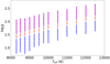 |
Fig. 2 Parameter coverage of the model atmosphere grid used in the present work. The different symbols refer to the microturbulent velocities ξ adopted in the computation of the models. Blue circles indicate ξ = 8 km s−1, black pluses 7 km s−1, red triangles 6 km s−1, green crosses5 km s−1, and magentadiamonds 4 km s−1. |
3.2 Effective temperature and surface gravity determination
We followed a well-established methodology to find the best solution for each object. First, by adopting Teff, we found the model that best reproduces the gravity sensitive features (the hydrogen Balmer lines; this step was repeated for different adopted Teff values, hence allowing us to define the locus of models for which the Balmer lines are equally well represented. We refer to this as the logg locus. In a similar fashion, but adopting the surface gravity, we identified the model that best reproduces the Teff sensitive features (see below). Repeating this step for different values of log g, we defined the Teff locus. Finally, the intersection of both lines defines the best possible solution for a given object in the Teff – logg plane (see Fig. 3).
At each step, we focussed on fitting individual lines. When fixing each effective temperature in our model grid to find the best-fitting surface gravity by means of a χ2 minimisation, we minimised the residuals between observed and synthetic Balmer lines Hα and Hβ1. Given the known correlation between the effective temperature and surface gravity, a linear relation with a positive slope is expected: for a higher Teff, we would need a higher log g to obtain the same strength of the lines. When finding Teff for an adopted logg value, we consider mostly metal lines as sensitive features. The strongest lines observed in our spectra correspond to He I and O I, for which the synthetic spectra are based on the model atoms of Przybilla (2005) and Przybilla et al. (2000), respectively. A linear relation between Teff and logg is again expected, thus the higher the assumed surface gravity, the higher the required effective temperature to reproduce the selected features. However, we did not find this linear relation for lower S/N spectra, with increasing noise giving rise to larger uncertainties. In addition to the lower S/N spectra, for decreasing Teff, the He I lines become weaker and eventually impossible to detect. For this reason, we also considered fitting the lines in the spectral region from 4950 to 5600 Å, since numerous metal lines are present. We fitted the best continuum between the model and data by means of a χ2 minimisation, and the strongest metal lines in the region. In the cases in which it was possible to do so (high S/N targets), for the sake of completeness, we checked that both fitting strategies provide the same stellar parameters within the error limits (as seen in Fig. 3). Examples of the fit provided by the best model are shown in Figs. 4–6 for H, He I, O I, and the 4950–5600 Å spectral window. Table 2 summarises the parameters derived in our analysis. We adopted a systematic error in Teff of 5%, and for logg (cgs) 0.10 dex, both reasonable estimations given the grid of the models and the quality of the data, see for example Kudritzki et al. (2008).
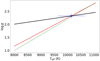 |
Fig. 3 Example of the method used to determine the temperature and surface gravity for star #151. The locus obtained by varying logg (in cgs units) for each fixed model-grid Teff in order to fit the hydrogen lines is shown by the solid black line. The loci obtained by varying Teff at each fixed model-grid logg in order to fit the He I and O I lines, and to fit the metal-line dominated 4950–5600 Å region, are indicated by the red-dashed and the green-dotted lines, respectively. The blue cross marks the intersection of the loci, yielding the adopted atmospheric parameter values. |
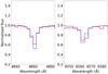 |
Fig. 4 Example for a best model fit to observed hydrogen lines for star #192. The observed spectrum is marked by the solid red line, and the model is shown by the blue-dashed line. |
3.3 Stellar luminosities, radii, and masses
With the fundamental stellar parameters Teff and logg at hand, we proceeded to derive luminosities L, spectroscopic masses Mspec, and radii R for the starsin our sample by combining observed magnitudes in different photometric bands with theoretical quantities obtained from the spectral energy distribution corresponding to the best-fitting models. A catalogue of observed Johnson B- and V -band magnitudes for sources in NGC 300, based on the work by Pietrzyński et al. (2001), was kindly provided by F. Bresolin (priv. comm.). The coordinates of the sources in this catalogue were cross-matched with our MUSE observations in order to extract the magnitudes for our targets. Coordinates and photometric magnitudes are reported in Table 1.
Individual reddening values E(B−V) were obtained by comparing observed and theoretical (B−V) colours from tailored models computed for the adopted atmospheric parameters. Bolometric corrections B.C. were also calculated from the tailored models. We adopted a standard value for the ratio of selective-to-total extinction RV = 3.1 to calculate the V -band extinction, and a tip of the red-giant branch (TRGB) distance to NGC 300 of d = 1.86 ± 0.07 Mpc as determined by Rizzi et al. (2006). Bolometric magnitudes Mbol were calculated from the extinction-corrected apparent V -band magnitude, the distance, and the B.C. for each object individually. The bolometric magnitudes were consecutively converted to stellar luminosities. Finally, from the combination of the stellar luminosities with the derived atmospheric parameters Teff and log g, stellar radii and spectroscopic masses were calculated.
Table 2 summarises all the derived properties of the stars in our sample. The table also presents the flux-weighted gravity of each star, gF =  , introduced by Kudritzki et al. (2003). We note that this quantity is a proxy for luminosity, as discussed in the aforementioned reference, and when normalised to the solar value, it represents the inverse of the quantity used by Langer & Kudritzki (2014) to define the spectroscopic Hertzsprung–Russell diagram (sHRD). The uncertainties presented in the table were calculated using Gaussian error propagation. For the observed magnitudes, we adopted the errors provided by Pietrzyński et al. (2001); the uncertainties affecting the intrinsic colours and bolometric corrections have a negligible effect on the final uncertainties.
Regarding the reddening values presented in Table 2, our stars show a wide range. However, disregarding the two stars with the highest values, the rest are consistent with the results presented by Kudritzki et al. (2008) for BA-type supergiant stars in NGC 300, as well as with the characteristic value for Cepheids based on optical and near-IR photometry by Gieren et al. (2005).
Atmospheric and stellar fundamental parameters for the sample stars.
3.4 Spectral type and luminosity class determination
The wavelength coverage of MUSE does not include the blue spectral region. Combined with the low S/N of the sample stars, a classical determination of spectral sub-types on a pure observational basis is not feasible here. Nevertheless, a model-based approach can be used; we applied the relationship between the spectral type and effective temperature as obtained by Firnstein & Przybilla (2012) based on Galactic BA supergiants. We have a few cases for which the derived effective temperatures are lower than the lowest average value for the coolest type in Firnstein & Przybilla (2012), A3. For these cases, we adopted either an A3 or A4 spectral type. Assigning a luminosity class LC to each object is also challenging. We resorted to the work by Firnstein (2010), which gives guidance to constrain the luminosity class from the stellar luminosity. Cases of LC II result from a reasonable extrapolation. The results are summarised in Table 2.
4 Discussion
4.1 Comparison with previous studies
A previous study of the same sample was presented by Roth et al. (2018). These authors analysed the stars by means of two different spectral libraries: (1) the empirical library MIUSCAT (unpublished, provided by Alexandre Vazdekis), and (2) a grid of PHOENIX models (Husser et al. 2013).
MIUSCAT is an extension of the MILES library (Sánchez-Blázquez et al. 2006; Cenarro et al. 2007; Falcón-Barroso et al. 2011). The library of PHOENIX models covers a range of 2300 K ≤Teff ≤ 12000 K and 0.0 ≤ logg ≤ 6.0 using the assumption of LTE. In both cases, the UlySS code (Koleva et al. 2009) based on pPXF (Cappellari & Emsellem 2004), initially developed for the study of stellar clusters, was used to find the best matching solution. Unlike the work presented here, Roth et al. (2018) proceeded to fit the full un-normalised spectra. In the case of hot massive stars, the main concern in terms of inaccuracy of their results would be the assumption of LTE.
Comparing our results with those by Roth et al. (2018), Teff values derived in both studies are consistent within the uncertainties for only eight stars (50% of our final sample), whilst in terms of logg this occurs in only four cases (25%). The tendency is for us to obtain higher gravities. These differences can be understood in terms of the very different methodology employed to analyse the stars, as well as the differences in the physical assumptions of the models. In addition, the MIUSCAT library has incomplete coverage of the HRD for hot stars (see discussion by Roth et al. 2018).
Regarding the spectral classification, we found four late B-type supergiants, ten early A-type stars (four of them supergiants and the rest bright giants), and two A4-type stars (with one supergiant and one bright giant). Comparing this with the previous classification, we resolved the A-types to a finer sub-class. On the other hand, Roth et al. (2018) found a broader range of luminosity classes, varying from II to Ia. This could be attributed to the very limited suitability of the empirical libraries for hot stars as pointed out above. The fact that the classification has been derived directly by model fitting while in our case we used the luminosity values of known stars as a reference could also explain our broader luminosity class range. We note, however, that the brightest supergiants in NGC 300, that is to say likely those of LC Ia, are of 18th mag (Bresolin et al. 2002), so 2–4 mag brighter than the stars investigated here.
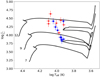 |
Fig. 7 HRD with evolutionary tracks for different masses (black solid lines, in M⊙) that account for rotation (Ekström et al. 2012). The red dots represent sample stars that move by more than 10% their evolutionary mass track position with respect to the sHRD in Fig. 8, and the blue squares are those that move less than 10%. |
4.2 Extending the flux-weighted gravity luminosity relationship (FGLR)
The FGLR was first derived by Kudritzki et al. (2003) as a new method for distance determination of supergiants:
 (1)
(1)
with a determined by the mass-luminosity relation (L ∝Mx) exponent x to a = 2.5x∕(1 − x). For massive stars, x ≈ 3 is found.
This relation holds for all supergiants and bright giants that have a constant luminosity track when they move to the right of the HRD. We can then use this relation to estimate the bolometric magnitudes, luminosities, and distances of supergiants and bright giants from which we only have spectral information. If we are able to resolve massive stars in distant galaxies, this can be a very powerful spectroscopic method to determine extragalactic distances.
To study the FGLR, we need to be sure that the stars are at the correct evolutionary stage. To verify that, we plotted the stars in relation to evolutionary tracks from Ekström et al. (2012) in the regular HRD (Fig. 7) and compared their position with respect to the tracks in the sHRD (Fig. 8).
The sHRD (Langer & Kudritzki 2014) shows the inverse of gF with respect to Teff. Using the sHRD, we can place the stars with only their spectroscopic information and without any knowledge of their distance or brightness. This provides an advantage to the HRD where we need to assume a distance to obtain the luminosities. In the HRD, if two stars with same Teff and L, but different masses (e.g. supergiants and post-AGB stars around log L∕L⊙ ~ 4), occupy the same location, they must have the same radius, so the log g has to be different. In the sHRD, the same degeneracy does not occur since the stars fall onto different iso-gravity lines, enabling us to discriminate them. Also multiple systems, where one star dominates the observed spectrum but other objects contribute to the total luminosity, can be discriminated.
We have defined a threshold of 10% of the star mass for the change in their relative position with respect to their evolutionary tracks in both diagrams, which is reasonable since it corresponds to their mass error. The red dots in Figs. 7 and 8 represent stars that move more than the 10% threshold, which indicates that they are not well-behaved objects. These are the same stars that show significantly larger spectroscopic than evolutionary masses that are derived from comparison with evolutionary tracks. The blue squares in Figs. 7 and 8 do not move by more than the threshold and a good correspondence between their spectral information and their true evolutionary stage and their single star status can be assumed. The latter stars are certain to be in the supergiant stage and hence the FGLR would hold.
To prove our last point, we considered our 16 stars along with the objects previously studied by Kudritzki et al. (2008) to derive the FLGR. As we can see in Fig. 9, the blue squares follow the old FGLR within their error limits. The initial FGLR gives the old parameters determined by Kudritzki et al. (2008): aold = − 3.52 and bold = 8.11. Adding the contribution of our newly found supergiants (blue squares in Fig. 9), we obtained a = −3.40 ± 0.04 and b = 8.02 ± 0.14. The results from this work are also in accordance with the new FGLR distance to NGC 300  = 26.34 ± 0.06 by Sextl et al. (2021).
As previously discussed, we performed the analysis with [Z] = 0.0 dex and [Z] = −0.15 dex, and although we found small systematic differences between the results, there is no observable effect on the derived flux-weighed gravities. This is due to the fact that Teff and logg are covariant; an increase in Teff requires an increase in logg, and vice versa. Hence, loggF does not effectively change (in particular given the uncertainties) and nor does the FGLR since the Teff changes are too small to introduce any effect on the derived reddening values.
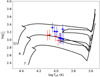 |
Fig. 8 Same as Fig. 7, but for the sHRD. The L′ is defined as the inverse of the flux-weighted gravity. The symbol encoding refers to movements relative to the tracks with respectto Fig. 7. |
4.3 Discrepant cases
As seen in Fig. 9, stars depicted by blue squares follow – within the uncertainties – the trend defined by the FGLR, whilst the ones represented by red dots deviate to some extent. We shall discuss these discrepant cases. For a star to lie above the relationship, under the consideration that it should not be there, either the derived luminosity is too high, or the flux-weighted gravity is too large (or both). The primary reason for the luminosity (bolometric magnitude) to be too high would be for the apparent magnitude to be too high. That could result from the fact that what is seen as a single star is in fact a combinationof several unresolved sources. In that case, it could well happen that whilst the most luminous star dominates the observed spectrum, one or several fainter sources could be contributing to the continuum, and hence the observed apparent magnitudes. Inspection of the MUSE datacube (see Fig. 1) results in that none of these objects show signs of being an extended source, which makes it unlikely that they are large star clusters. On the other hand, it cannot be ruled out that they are small stellar aggregates that are not resolvable at the distance of NGC 300.
An alternative explanation for this deviation is that as we increase the log gF and move to the bottom left of the FGLR, the stars decrease in mass. Population simulations predict that the FGLR will get wider for lower masses, as discussed by Meynet et al. (2015). We expect the density of objects to increase as the masses decrease because of the so-called initial mass function (IMF) effect: we always expect to find a higher number of low mass stars than of massive stars (e.g. Salpeter 1955; Kroupa 2001), widening the FGLR because of the increased scatter.
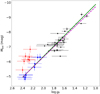 |
Fig. 9 FGLR for the stars in NGC 300. Black symbols denote the stars studied by Kudritzki et al. (2008), with the corresponding FGLR regression line marked in solid green. Blue and red symbols mark the stars analysed here, with the magenta-dashed line representing the regression line derived from the black and blue symbols. |
5 Outlook
A quantitative analysis of 16 BA-type supergiants and bright giants in NGC 300 based on VLT/MUSE integral field spectroscopy was performed here, with a focus on determining basic atmospheric and fundamental stellar parameters. This allowed us to verify that the FGLR can be extended towards less luminous stars than studied before. However, the study has faced limitations by the rather restricted S∕N ≲ 20 of the spectra. For future work, longer exposures and use of the currently available AO mode of MUSE should be aimed at boosting the S/N and improving the spatial resolution. This would not only facilitate a similar study as the one performed here to be achieved at much reduced uncertainties, but this would also help to determine metallicities and likely elemental abundances for selected individual chemical elements. The full potential of MUSE for extragalactic stellar astrophysics could thus be demonstrated. Studies with increased scientific value could be made once the BlueMUSE medium-resolution panoramic integral field spectrograph becomes operational, which has been proposed as a new instrument for the VLT (Richard et al. 2019). BlueMUSE is optimised for the optical blue, where most of the diagnostic spectral features of hot supergiants are located.
Acknowledgements
We would like to thank the referee for useful comments which helped improve the paper. Based on observations collected at the European Southern Observatory under ESO programme 094.D-0116(A). The authors want to thank Tim-Oliver Husser, Benjamin Giesers and Fabio Bresolin for valuable input. GGT acknowledges funding by a scholarship within the Erasmus Mundus Joint Master Degree programme AstroMundus. S.K. acknowledges funding from UKRI in the form of a Future Leaders Fellowship (grant no. MR/T022868/1). N.C. acknowledges funding from the Deutsche Forschungsgemeinschaft (DFG) - CA 2551/1-1.
References
- Andrews, B. H., & Martini, P. 2013, ApJ, 765, 140 [NASA ADS] [CrossRef] [Google Scholar]
- Appenzeller, I., Fricke, K., Fürtig, W., et al. 1998, The Messenger, 94, 1 [NASA ADS] [Google Scholar]
- Baade, W. 1944, ApJ, 100, 137 [NASA ADS] [CrossRef] [Google Scholar]
- Bacon, R., Vernet, J., Borisova, E., et al. 2014, The Messenger, 157, 13 [NASA ADS] [Google Scholar]
- Berger, T. A., Kudritzki, R.-P., Urbaneja, M. A., et al. 2018, ApJ, 860, 130 [CrossRef] [Google Scholar]
- Bodensteiner, J., Sana, H., Mahy, L., et al. 2020, A&A, 634, A51 [NASA ADS] [CrossRef] [EDP Sciences] [Google Scholar]
- Bresolin, F., Kudritzki, R.-P., Mendez, R. H., & Przybilla, N. 2001, ApJ, 548, L159 [NASA ADS] [CrossRef] [Google Scholar]
- Bresolin, F., Gieren, W., Kudritzki, R.-P., Pietrzyński, G., & Przybilla, N. 2002, ApJ, 567, 277 [NASA ADS] [CrossRef] [Google Scholar]
- Bresolin, F., Pietrzyński, G., Gieren, W., et al. 2004, ApJ, 600, 182 [NASA ADS] [CrossRef] [Google Scholar]
- Bresolin, F., Gieren, W., Kudritzki, R.-P., et al. 2009, ApJ, 700, 309 [NASA ADS] [CrossRef] [Google Scholar]
- Bresolin, F., Kudritzki, R.-P., Urbaneja, M. A., et al. 2016, ApJ, 830, 64 [NASA ADS] [CrossRef] [Google Scholar]
- Cappellari, M., & Emsellem, E. 2004, PASP, 116, 138 [Google Scholar]
- Castro, N., Urbaneja, M. A., Herrero, A., et al. 2012, A&A, 542, A79 [NASA ADS] [CrossRef] [EDP Sciences] [Google Scholar]
- Castro, N., Crowther, P. A., Evans, C. J., et al. 2018, A&A, 614, A147 [NASA ADS] [CrossRef] [EDP Sciences] [Google Scholar]
- Castro, N., Crowther, P. A., Evans, C. J., et al. 2021, A&A, 648, A65 [NASA ADS] [CrossRef] [EDP Sciences] [Google Scholar]
- Cenarro, A. J., Peletier, R. F., Sanchez-Blazquez, P., et al. 2007, VizieR Online Data Catalog: J/MNRAS/374/664 [Google Scholar]
- Ekström, S., Georgy, C., Eggenberger, P., et al. 2012, A&A, 537, A146 [Google Scholar]
- Falcón-Barroso, J., Sánchez-Blázquez, P., Vazdekis, A., et al. 2011, A&A, 532, A95 [Google Scholar]
- Firnstein, M. 2010, PhD thesis, University of Erlangen-Nuremberg, Germany [Google Scholar]
- Firnstein, M., & Przybilla, N. 2012, A&A, 543, A80 [NASA ADS] [CrossRef] [EDP Sciences] [Google Scholar]
- Gazak, J. Z., Kudritzki, R., Evans, C., et al. 2015, ApJ, 805, 182 [NASA ADS] [CrossRef] [Google Scholar]
- Gieren, W., Pietrzyński, G., Soszyński, I., et al. 2005, ApJ, 628, 695 [NASA ADS] [CrossRef] [Google Scholar]
- Groth, H. G. 1961, Z. Astrophys., 51, 231 [NASA ADS] [Google Scholar]
- Hosek, M. W. J., Kudritzki, R.-P., Bresolin, F., et al. 2014, ApJ, 785, 151 [NASA ADS] [CrossRef] [Google Scholar]
- Hubble, E. P. 1929, ApJ, 69, 103 [NASA ADS] [CrossRef] [Google Scholar]
- Humphreys, R. M., & Aaronson, M. 1987, AJ, 94, 1156 [CrossRef] [Google Scholar]
- Humphreys, R. M., & Davidson, K. 1979, ApJ, 232, 409 [Google Scholar]
- Husser, T. O., Wende-von Berg, S., Dreizler, S., et al. 2013, A&A, 553, A6 [NASA ADS] [CrossRef] [EDP Sciences] [Google Scholar]
- Kamann, S., Wisotzki, L., & Roth, M. M. 2013, A&A, 549, A71 [NASA ADS] [CrossRef] [EDP Sciences] [Google Scholar]
- Karachentsev, I. D., Grebel, E. K., Sharina, M. E., et al. 2003, A&A, 404, 93 [CrossRef] [EDP Sciences] [Google Scholar]
- Kewley, L. J.,& Ellison, S. L. 2008, ApJ, 681, 1183 [NASA ADS] [CrossRef] [Google Scholar]
- Koleva, M., Prugniel, P., Bouchard, A., & Wu, Y. 2009, A&A, 501, 1269 [CrossRef] [EDP Sciences] [Google Scholar]
- Kroupa, P. 2001, MNRAS, 322, 231 [NASA ADS] [CrossRef] [Google Scholar]
- Kudritzki, R. P., Lennon, D. J., & Puls, J. 1995, in Science with the VLT (Berlin: Springer), 246 [CrossRef] [Google Scholar]
- Kudritzki, R. P., Bresolin, F., & Przybilla, N. 2003, ApJ, 582, L83 [Google Scholar]
- Kudritzki, R. P., Urbaneja, M. A., Bresolin, F., et al. 2008, ApJ, 681, 269 [NASA ADS] [CrossRef] [Google Scholar]
- Kudritzki, R.-P., Urbaneja, M. A., Gazak, Z., et al. 2012, ApJ, 747, 15 [CrossRef] [Google Scholar]
- Kudritzki, R.-P., Urbaneja, M. A., Gazak, Z., et al. 2013, ApJ, 779, L20 [NASA ADS] [CrossRef] [Google Scholar]
- Kudritzki, R.-P., Urbaneja, M. A., Bresolin, F., Hosek, M. W., & Przybilla, N. 2014, ApJ, 788, 56 [NASA ADS] [CrossRef] [Google Scholar]
- Kudritzki, R. P., Castro, N., Urbaneja, M. A., et al. 2016, ApJ, 829, 70 [NASA ADS] [CrossRef] [Google Scholar]
- Langer, N., & Kudritzki, R. P. 2014, A&A, 564, A52 [NASA ADS] [CrossRef] [EDP Sciences] [Google Scholar]
- Lequeux, J., Peimbert, M., Rayo, J. F., Serrano, A., & Torres-Peimbert, S. 1979, A&A, 500, 145 [NASA ADS] [Google Scholar]
- Makarov, D., Prugniel, P., Terekhova, N., Courtois, H., & Vauglin, I. 2014, A&A, 570, A13 [NASA ADS] [CrossRef] [EDP Sciences] [Google Scholar]
- McCarthy, J. K., Lennon, D. J., Venn, K. A., et al. 1995, ApJ, 455, L135 [NASA ADS] [Google Scholar]
- Meynet, G., Kudritzki, R. P., & Georgy, C. 2015, A&A, 581, A36 [NASA ADS] [CrossRef] [EDP Sciences] [Google Scholar]
- Oke, J. B., Cohen, J. G., Carr, M., et al. 1995, PASP, 107, 375 [Google Scholar]
- Pietrzyński, G., Gieren, W., Fouqué, P., & Pont, F. 2001, A&A, 371, 497 [NASA ADS] [CrossRef] [EDP Sciences] [Google Scholar]
- Pietrzyński, G., Gieren, W., Fouqué, P., & Pont, F. 2002, AJ, 123, 789 [CrossRef] [Google Scholar]
- Przybilla, N. 2002, PhD thesis, Ludwig-Maximilians-Universität, München, Germany [Google Scholar]
- Przybilla, N. 2005, A&A, 443, 293 [NASA ADS] [CrossRef] [EDP Sciences] [Google Scholar]
- Przybilla, N., & Butler, K. 2004, ApJ, 609, 1181 [NASA ADS] [CrossRef] [Google Scholar]
- Przybilla, N., Butler, K., Becker, S. R., Kudritzki, R. P., & Venn, K. A. 2000, A&A, 359, 1085 [NASA ADS] [Google Scholar]
- Przybilla, N., Butler, K., Becker, S. R., & Kudritzki, R. P. 2006, A&A, 445, 1099 [NASA ADS] [CrossRef] [EDP Sciences] [Google Scholar]
- Przybylski, A. 1968, MNRAS, 139, 313 [NASA ADS] [CrossRef] [Google Scholar]
- Przybylski, A. 1971, MNRAS, 152, 197 [CrossRef] [Google Scholar]
- Przybylski, A. 1972, MNRAS, 159, 155 [CrossRef] [Google Scholar]
- Richard, J., Bacon, R., Blaizot, J., et al. 2019, ArXiv e-prints, [arXiv:1906.01657] [Google Scholar]
- Rizzi, L., Bresolin, F., Kudritzki, R. P., Gieren, W., & Pietrzyński, G. 2006, ApJ, 638, 766 [NASA ADS] [CrossRef] [Google Scholar]
- Roth, M. M., Sandin, C., Kamann, S., et al. 2018, A&A, 618, A3 (Paper I) [NASA ADS] [CrossRef] [EDP Sciences] [Google Scholar]
- Salpeter, E. E. 1955, ApJ, 121, 161 [Google Scholar]
- Sánchez-Blázquez, P., Peletier, R. F., Jiménez-Vicente, J., et al. 2006, MNRAS, 371, 703 [Google Scholar]
- Sextl, E., Kudritzki, R.-P., Weller, J., Urbaneja, M. A., & Weiss, A. 2021, ApJ, 914, 94 [CrossRef] [Google Scholar]
- Tremonti, C. A., Heckman, T. M., Kauffmann, G., et al. 2004, ApJ, 613, 898 [Google Scholar]
- U, V., Urbaneja, M. A., Kudritzki, R.-P., et al. 2009, ApJ, 704, 1120 [CrossRef] [Google Scholar]
- Urbaneja, M. A., Herrero, A., Bresolin, F., et al. 2003, ApJ, 584, L73 [Google Scholar]
- Urbaneja, M. A., Herrero, A., Bresolin, F., et al. 2005, ApJ, 622, 862 [Google Scholar]
- Urbaneja, M. A., Kudritzki, R.-P., Bresolin, F., et al. 2008, ApJ, 684, 118 [NASA ADS] [CrossRef] [Google Scholar]
- Urbaneja, M. A., Kudritzki, R. P., Gieren, W., et al. 2017, AJ, 154, 102 [NASA ADS] [CrossRef] [Google Scholar]
- Venn, K. A. 1995a, ApJS, 99, 659 [NASA ADS] [CrossRef] [Google Scholar]
- Venn, K. A. 1995b, ApJ, 449, 839 [NASA ADS] [CrossRef] [Google Scholar]
- Venn, K. A. 1999, ApJ, 518, 405 [Google Scholar]
- Venn, K. A., McCarthy, J. K., Lennon, D. J., et al. 2000, ApJ, 541, 610 [NASA ADS] [CrossRef] [Google Scholar]
- Venn, K. A., Lennon, D. J., Kaufer, A., et al. 2001, ApJ, 547, 765 [NASA ADS] [CrossRef] [Google Scholar]
- Venn, K. A., Tolstoy, E., Kaufer, A., et al. 2003, AJ, 126, 1326 [NASA ADS] [CrossRef] [Google Scholar]
- Verdugo, E., Talavera, A., & Gómez de Castro, A. I. 1999, A&AS, 137, 351 [NASA ADS] [CrossRef] [EDP Sciences] [Google Scholar]
- Weilbacher, P. M., Palsa, R., Streicher, O., et al. 2020, A&A, 641, A28 [NASA ADS] [CrossRef] [EDP Sciences] [Google Scholar]
- Wofford, A., Ramírez, V., Lee, J. C., et al. 2020, MNRAS, 493, 2410 [NASA ADS] [CrossRef] [Google Scholar]
- Wolf, B. 1972, A&A, 20, 275 [NASA ADS] [CrossRef] [Google Scholar]
- Wolf, B. 1973, A&A, 28, 335 [NASA ADS] [Google Scholar]
Unlike in previous applications of the models, our MUSE data only cover Hα and Hβ, which may be influenced by a sufficiently strong stellar wind. However, at the comparatively low luminosities of the target stars, the two lines are expected to be symmetric, that is overall unaffected by mass outflow, as a comparison with high-resolution spectra of analogous Galactic objects shows (Verdugo et al. 1999). Consequently, they are represented well by the hydrostatic approach and the synthetic non-LTE profiles based on the hydrogen model atom by Przybilla & Butler (2004).
All Tables
All Figures
|
Fig. 1 Chart of NGC 300 field (i) with the programme stars marked in red and their ID numbers in blue (according to Paper I). The image is stacked over all recorded wavelengths in the datacube. |
| In the text | |
|
Fig. 2 Parameter coverage of the model atmosphere grid used in the present work. The different symbols refer to the microturbulent velocities ξ adopted in the computation of the models. Blue circles indicate ξ = 8 km s−1, black pluses 7 km s−1, red triangles 6 km s−1, green crosses5 km s−1, and magentadiamonds 4 km s−1. |
| In the text | |
|
Fig. 3 Example of the method used to determine the temperature and surface gravity for star #151. The locus obtained by varying logg (in cgs units) for each fixed model-grid Teff in order to fit the hydrogen lines is shown by the solid black line. The loci obtained by varying Teff at each fixed model-grid logg in order to fit the He I and O I lines, and to fit the metal-line dominated 4950–5600 Å region, are indicated by the red-dashed and the green-dotted lines, respectively. The blue cross marks the intersection of the loci, yielding the adopted atmospheric parameter values. |
| In the text | |
|
Fig. 4 Example for a best model fit to observed hydrogen lines for star #192. The observed spectrum is marked by the solid red line, and the model is shown by the blue-dashed line. |
| In the text | |
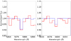 |
Fig. 5 Same as Fig. 4, but for He I lines. |
| In the text | |
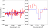 |
Fig. 6 Same as Fig. 4, but for the region from 4950–5600 Å (left panel), and for O I (right panel). |
| In the text | |
|
Fig. 7 HRD with evolutionary tracks for different masses (black solid lines, in M⊙) that account for rotation (Ekström et al. 2012). The red dots represent sample stars that move by more than 10% their evolutionary mass track position with respect to the sHRD in Fig. 8, and the blue squares are those that move less than 10%. |
| In the text | |
|
Fig. 8 Same as Fig. 7, but for the sHRD. The L′ is defined as the inverse of the flux-weighted gravity. The symbol encoding refers to movements relative to the tracks with respectto Fig. 7. |
| In the text | |
|
Fig. 9 FGLR for the stars in NGC 300. Black symbols denote the stars studied by Kudritzki et al. (2008), with the corresponding FGLR regression line marked in solid green. Blue and red symbols mark the stars analysed here, with the magenta-dashed line representing the regression line derived from the black and blue symbols. |
| In the text | |
Current usage metrics show cumulative count of Article Views (full-text article views including HTML views, PDF and ePub downloads, according to the available data) and Abstracts Views on Vision4Press platform.
Data correspond to usage on the plateform after 2015. The current usage metrics is available 48-96 hours after online publication and is updated daily on week days.
Initial download of the metrics may take a while.