| Issue |
A&A
Volume 656, December 2021
|
|
|---|---|---|
| Article Number | A59 | |
| Number of page(s) | 16 | |
| Section | Cosmology (including clusters of galaxies) | |
| DOI | https://doi.org/10.1051/0004-6361/202141540 | |
| Published online | 03 December 2021 | |
Deep Chandra observations of merging galaxy cluster ZwCl 2341+0000
1
Leiden Observatory, Leiden University, PO Box 9513 2300 RA Leiden, The Netherlands
e-mail: xyzhang@strw.leidenuniv.nl
2
SRON Netherlands Institute for Space Research, Niels Bohrweg 4, 2333 CA Leiden, The Netherlands
3
Kavli Institute for the Physics and Mathematics of the Universe (WPI), The University of Tokyo, Kashiwa, Chiba 277-8583, Japan
4
Dipartimento di Fisica e Astronomia, Università di Bologna, Via Gobetti 93/2, 40122 Bologna, Italy
5
INAF – Istituto di Radioastronomia di Bologna, Via Gobetti 101, 40129 Bologna, Italy
6
University of Hamburg, Hamburger Sternwarte, Gojenbergsweg 112, 21029 Hamburg, Germany
7
Harvard-Smithsonian Center for Astrophysics, 60 Garden Street, Cambridge, MA 02138, USA
8
Department of Physics, Rikkyo University, 3-34-1 Nishi-Ikebukuro, Toshima-ku, Tokyo 171-8501, Japan
Received:
14
June
2021
Accepted:
29
September
2021
Context. Knowledge of X-ray shock and radio relic connection in merging galaxy clusters has been greatly extended in terms of both observation and theory over the last decade. ZwCl 2341+0000 is a double-relic merging galaxy cluster; previous studies have shown that half of the southern relic is associated with an X-ray surface brightness discontinuity, while the other half not. The discontinuity was believed to be a shock front. Therefore, it is a mysterious case of an only partial shock-relic connection.
Aims. By using the 206.5 ks deep Chandra observations, we aim to investigate the nature of the southern surface brightness discontinuity. Meanwhile, we aim to explore new morphological and thermodynamical features.
Methods. We perform both imaging and spectroscopic analyses to investigate the morphological and thermodynamical properties of the cluster. In addition to the X-ray data, we utilize the GMRT 325 MHz image and JVLA 1.5 GHz and 3.0 GHz images to compute radio spectral index maps.
Results. Surface brightness profile fitting and the temperature profile suggest that the previously reported southern surface brightness discontinuity is better described as a sharp change in slope or as a kink. This kink is likely contributed by the disrupted core of the southern subcluster. The radio spectral index maps show spectral flattening at the south-eastern edge of the southern relic, suggesting that the location of the shock front is 640 kpc away from the kink, where the X-ray emission is too faint to detect a surface brightness discontinuity. We update the radio shock Mach number to be ℳradio, S = 2.2 ± 0.1 and ℳradio, N = 2.4 ± 0.4 for the southern and northern radio relics based on the injection spectral indices. We also put a 3σ lower limit on the X-ray Mach number of the southern shock to be ℳX-ray, S > 1.6. Meanwhile, the deep observations reveal that the northern subcluster is in a perfect cone shape, with a ∼400 kpc linear cold front on each side. This type of conic subcluster has been predicted by simulations but is observed here for the first time. It represents a transition stage between a blunt-body cold front and a slingshot cold front. Strikingly, we found a 400 kpc long gas trail attached to the apex of the cone, which could be due to the gas stripping. In addition, an over-pressured hot region is found in the south-western flank of the cluster.
Key words: X-rays: galaxies: clusters / galaxies: clusters: intracluster medium / galaxies: clusters: individual: ZwCl 2341+0000 / shock waves
© ESO 2021
1. Introduction
As the nodes of the large-scale structures in the Universe, galaxy clusters grow hierarchically by accreting gas from cosmic filaments and merging with subclusters. Major galaxy cluster mergers are the most dramatic events in the Universe, releasing energies of up to 1064 erg. During the merger, the intracluster medium (ICM) that belongs to each subcluster is mixed and shows a disturbed X-ray morphology. Two types of surface brightness jumps, shock fronts and contact discontinuities, are discovered in both observations (e.g., Vikhlinin et al. 2001; Markevitch et al. 2002; Owers et al. 2009; Ghizzardi et al. 2010; Botteon et al. 2018) and simulations (e.g., Ascasibar & Markevitch 2006; ZuHone 2011) of merging clusters.
Since the first report of the association of an X-ray shock and a radio relic (Finoguenov et al. 2010) – which is a type of morphologically elongated, spectrally steep, and polarized diffuse radio source observed in galaxy cluster peripheries – dozens of radio relics have been confirmed to be associated with shock fronts (see the review of van Weeren et al. 2019). The Mach number of shock fronts can be estimated either by radio observations based on the assumption of the diffusive shock acceleration (DSA) theory (e.g., Krymskii 1977; Bell 1978; Blandford & Ostriker 1978) or by X-ray observations based on the Rankine-Hugoniot condition (Landau & Lifshitz 1959). The Mach numbers estimated from radio observations are systematically higher than those based on X-ray observations (van Weeren et al. 2019), which could be due to the projection effects (Hong et al. 2015) or the propagation of shocks through a magnetized turbulent ICM (Dominguez-Fernandez et al. 2021). Nevertheless, most of the merging shocks are in low Mach numbers (ℳ ≲ 3), which challenge the acceleration efficiency of the current DSA theory. Therefore, galaxy clusters are unique laboratories for investigating the particle acceleration of weak shocks.
In contrast to shock fronts, contact discontinuities, also known as cold fronts, are sharp surface brightness and temperature edges that hold pressure equilibrium. The cold fronts in merging clusters are usually “remnant core” cold fronts (Tittley & Henriksen 2005), that is, the cores of the original subclusters, and are undergoing ram-pressure stripping (Gunn & Gott 1972). Typically, the remnant cores are in the shape of blunt bodies, for example, Bullet Cluster (Markevitch et al. 2002) and Abell 2146 (Russell et al. 2010). By studying the cold fronts with the subarcsecond spatial resolution of Chandra, knowledge of transport processes and the effect of magnetic fields in the ICM has been well developed (Markevitch & Vikhlinin 2007; Zuhone & Roediger 2016).
ZwCl 2341+0000 (z = 0.27) is a merging galaxy cluster that hosts radio relics in its southern and northern peripheries (van Weeren et al. 2009). The presence of the double relics usually suggests a binary merger with a simple merging geometry and a small angle between the merging axis and the plane of the sky. This merging axis angle was later confirmed to be  by Benson et al. (2017). The diffuse radio emission of ZwCl 2341+0000 was first reported by Bagchi et al. (2002) in the 327 MHz Very Large Array (VLA) image and 1.4 GHz NRAO VLA Sky Survey (NVSS) image. The two relics (denoted RN and RS) were later resolved in Giant Metrewave Radio Telescope (GMRT) 610 MHz, 241 MHz, and 157 MHz observations, where the radio halo is absent (van Weeren et al. 2009). The southern relic consists of three different components (RS1–3). By using a VLA 1.4 GHz D-configuration observation, Giovannini et al. (2010) discovered large-scale filamentary diffuse emission along the entire cluster after removing point sources, which implies the possible presence of a radio halo. In optical frequencies, the galaxy distribution is NW-SE elongated. The dynamical mass of the system was first estimated to be ∼1 − 3 × 10¹⁵ M⊙ (Boschin et al. 2013). Later, Benson et al. (2017) pointed out that the dynamical mass is biased in this complex merging system, and, by using weak lensing, they reported a mass estimation of (5.57 ± 2.47)×1014 M⊙, which is consistent with the mass estimation made using the Sunyaev-Zel’dovich (SZ) effect by Planck, MSZ = (5.2 ± 0.4)×1014 M⊙ (Planck Collaboration XXVII 2016). Moreover, the optical analysis favors a three-subcluster model by using the Gaussian mixture model method, where a third subcluster with a different redshift (z = 0.27432) is spatially overlaid on the northern subcluster. The northern and southern subclusters are at redshifts of 0.26866 and 0.26844, respectively (Benson et al. 2017).
Ogrean et al. (2014) studied the radio-X-ray connection at the radio relics using Chandra and XMM-Newton observations. They detected X-ray surface brightness discontinuities at both the southern and northern radio relics. The discontinuities were believed to be shock fronts, although spectral analysis was not possible due to the shallow observations. Ogrean et al. (2014) also found that only half of the southern radio relic is associated with X-ray surface brightness discontinuities. This was the original intention of obtaining the additional observations that are presented in this paper. The deep Chandra observations not only unravel the previous mystery but also reveal new striking morphological features, for example, a cone-shaped subcluster that is predicted by simulations but had never before been observed. These new discoveries are explicitly described and discussed in the subsequent sections.
In this paper we present the results of the deep Chandra observations of ZwCl 2341+0000. In addition, we utilized radio observations performed with the GMRT at 325 MHz as well as the Jansky Very Large Array (JVLA) L-band (1−2 GHz) B and C configurations and S-band (2−4 GHz) C and D configurations (published by Benson et al. 2017) to compute spectral index maps and probe the properties of the shock fronts. The organization of this paper is as follows. In Sect. 2 we present the details of the X-ray and radio observations, data reduction and data analysis. The detailed analysis results for each region of interest are presented in Sect. 3. We discuss and conclude the work in Sects. 4 and 5. We adopt a Λ cold dark matter universe with cosmological parameters ΩΛ = 0.7, Ω0 = 0.3, and H0 = 70 km s−1 Mpc−1. At z = 0.27, one arcminute corresponds to a physical size of 248 kpc.
2. Observation and data analysis
2.1. Chandra X-ray data
ZwCl 2341+0000 was observed by the Chandra Advanced CCD Imaging Spectrometer (ACIS) five times (see Table 1 for details). We used the Chandra Interactive Analysis of Observations (CIAO) v4.12 (Fruscione et al. 2006) and CALDB v4.9.2 for data reduction. All level-1 event files were reprocessed by the task chandra_repro with VFAINT mode background event filtering. Flare state events were filtered from the level-2 event files by using lc_clean. The total filtered exposure time is 206.5 ks.
Details of the Chandra observations.
We used stowed background files to estimate the non-X-ray background (NXB). All stowed background event files are combined and reprocessed by the task acis_process_events using the latest gain calibration files. The stacked stowed background of each ACIS-I chip has a total exposure time of 1.02 Ms. For each ObsID, we scaled the NXB such that the 9−12 keV count rate matches the observation. The uncertainty of each scaling factor is calculated as the standard deviation of the scaling factors of individual ACIS-I chips, which is listed in the last column of Table 1.
2.1.1. Imaging analysis
We extracted and combined the 0.5−2.0 keV count images using merge_obs. The exposure maps are calculated using a weighted spectrum file generated by make_instmap_weighted, where the spectral model is a single Astrophysical Plasma Emission Code (APEC) model with kT = 5 keV, which is the averaged temperature measured by Suzaku (Akamatsu & Kawahara 2013). The non X-ray background (NXB) count images were generated from the stowed observation files described in Sect. 2. After applying the combined exposure map to the NXB-subtracted count image, we obtained the final X-ray flux map (see Fig. 1).
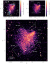 |
Fig. 1. Top left: X-ray flux map in the 0.5−2.0 keV band convolved with a σ = 1.97″ (four pixel) Gaussian kernel. Overlaid are the JVLA C-array 1.5 GHz radio contours at [1, 2, 4]×0.075 mJy beam−1. The terms of the relic sources RS-1–3 and RN are introduced by van Weeren et al. (2009). Identified point sources that overlap with the southern relic are marked by cyan boxes. Top right: image from which point sources have been removed. Surface brightness features are labeled. The locations of the three brightest cluster galaxies adopted from Benson et al. (2017) are marked as cyan crosses. Bottom: extraction regions used for detailed X-ray analysis in Sect. 3. For the regions SE edge, SW bays, western wing, and NE wing, the individual temperature bins in Fig. 6 are plotted. The arrows beside each bin indicate the directions of the profiles. |
Point sources were detected from the unbinned count image by using the task wavdetect with wavelet scales of 1.0, 2.0, 4.0, 8.0, and 16.0 pixels. The parameter sigthresh was set to 10−6. The output region file is used for masking point sources in both imaging and spectral analysis. Meanwhile, we used the task roi to generate background regions around detected point sources and used the task dmfilth to create an image containing only the diffuse emission. We note that the point source subtracted image can better illustrate the surface brightness features, but the flux in point source regions is interpolated from the ambient background regions, which is not the exact value of the ICM emission at the respective location. Therefore, in both imaging and spectroscopic analyses, we excluded the point sources using the region files from wavdetect.
We extracted surface brightness profiles and fitted them using the Sbfit1 v0.2.0 package (Zhang 2021). The package uses a forward fitting strategy together with C-statistics (Cash 1979).
2.1.2. Spectral analysis
We used the task specextract to extract source and NXB spectra and create the corresponding weighted ancillary response files (ARFs) and response matrix files (RMFs). We used the spectral fitting package SPEX v3.06 (Kaastra et al. 1996, 2020) for spectral analysis. The original format spectra and response files were converted to SPEX format by the trafo task. We fit the spectra in the 0.5−7.0 keV band. All spectra were optimally binned (Kaastra & Bleeker 2016) and fitted with C-statistics (Cash 1979; Kaastra 2017). The reference proto-solar element abundance table is from Lodders et al. (2009). By using Pyspextools (de Plaa 2020), the NXB spectra were first smoothed by a Wiener filter with a window length of seven spectral channels and then subtracted from the source spectra. We fit the spectra of the five observations simultaneously.
The source spectra are modeled using a spectral component combination of cie1 + (cie2 + pow)×hot + cie3 × red × hot, where cie 1–3 are the single temperature collisional ionization equilibrium (CIE) models for the local hot bubble (LHB), galactic halo (GH), and the ICM; for cie3, the abundances of elements from Li to Mn are fixed to 0.3 Z⊙, which is the averaged value of this cluster (see Sect. 3.1). While for cie 1 and 2, all abundances are fixed to the proto-solar abundance. The power law model for the cosmic X-ray background (CXB) residual is denoted as “pow” and its photon index is fixed to 1.41. The model red denotes the redshift of the cluster, which is fixed to 0.27. The hot is the CIE absorption model, where the temperature is fixed to 5 × 10⁻⁴ keV to represent the absorption from the Galactic neutral gas, and the column density is fixed to nH = 3.7 × 1020 cm−2, which is from the tool nhtot2 (Willingale et al. 2013). Details of the modeling of LHB, GH, and CXB residual are described in Sect. 2.1.3.
2.1.3. X-ray background modeling
We used the ROSAT All-Sky Survey (RASS) spectra as a reference to study the X-ray foreground components. The spectrum of an 0.3° −1.0° annulus centered at the cluster was extracted using the ROSAT X-Ray Background Tool (Sabol & Snowden 2019). Similar to the source spectra, we fit the ROSAT background spectrum using a spectral model combination of cie1 + hot × (cie2 + pow). To solve the degeneracy of the LHB and GH temperatures, we fixed the LHB temperature to a typical value of 0.1 keV (e.g., Kuntz & Snowden 2000). The best-fit values are listed in Table 3.
Meanwhile, we extracted spectra from an offset region outside the cluster’s r500 to cross-check the foreground component (see Fig. 2). The spectral components are the same as those of the RASS spectrum. Because the effective area of Chandra drops dramatically below 1 keV, the LHB component cannot be constrained. We fixed the temperature and normalization of the LHB component to the values of the RASS spectrum. The best-fit results of the Chandra offset spectra are listed in Table 3 as well. Though with large uncertainties, the normalization as well as the temperature of the GH component are consistent to the values of the RASS spectrum fit. Therefore, in the source spectral analysis, we fixed the parameters of LHB and GH to the values of the RASS spectrum and fixed the parameters of the CXB residual to the value of the Chandra offset spectra.
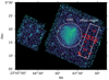 |
Fig. 2. Illustration of the offset extraction region, which is the white rectangle. Point-like sources are excluded using red regions, including the red rectangle, which is used to collectively exclude a series of observed clumps. The dashed circle is the r500 region of the cluster, which is centered at [23:43:42.1, +00:17:49.9]. |
2.1.4. Systematic uncertainty estimation
The GH and CXB residual components as well as the scaling factor of the NXB can introduce uncertainties in the fit results. The best-fit normalization of the GH in the Chandra offset spectrum is 20% different from the value of the RASS spectrum. Therefore, we use 20% to estimate the uncertainty introduced by the GH component. For the CXB residual, converted to the 2−8 keV band, the surface brightness is 1.8 × 10⁻¹⁵ erg s−1 cm2 arcmin−2. Using Eqs. (C.4) and (C.5) in Zhang et al. (2020) and assuming the log N − log S relation is identical to the Chandra Deep Field South (Lehmer et al. 2012), the corresponding point source exclusion limit is 3 × 10⁻¹⁵ erg s−1 cm−2 and the CXB residual uncertainty on a 1 arcmin2 area is 57%. For any of the spectra in the analysis, the CXB residual uncertainty is scaled from 57% by a factor of A−1/2, where A is the extraction area converted from the backscal value in the spectrum header. The largest NXB uncertainty amounts to 3% in ObsID 18073; therefore, we conservatively used 3% to estimate the NXB systematic uncertainty for all five observations.
By fitting the spectra extracted inside r500, which include most of the ICM photons, we find that the statistical uncertainty is larger than the systematic uncertainties from the GH and CXB by an order of magnitude, and is larger than the NXB systematic uncertainty by four orders of magnitude. We also checked the systematic uncertainties in two smaller regions, the LK1 and HT3 regions in the thermodynamic maps (see Fig. 3), which are in a high and a low surface brightness, respectively. In the LK1 region, the statistical uncertainty is larger than all other systematic uncertainties by over an order of magnitude. In the HT3 region, the systematic uncertainties increase due to the low surface brightness of the ICM emission. Nevertheless, the statistical uncertainty is still a factor of four larger than the systematic uncertainty contributed by GH, and over an order of magnitude higher than other systematic uncertainties. The one-fourth of the additional uncertainty will result in a 3% increase after uncertainty propagation. Therefore, in this work, we only present statistical uncertainties.
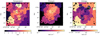 |
Fig. 3. Temperature, pseudo pressure, and entropy maps of ZwCl 2341+0000, overlaid with the X-ray surface brightness contours. High temperature and low entropy regions are labeled as HT1–4 and LK1–3, respectively. |
2.1.5. Thermodynamic maps
To create spatial bins for temperature, pseudo pressure, and entropy maps, we used the tool contbin3 (Sanders 2006). The signal to noise ratio was set to 30 and the geometric constraint was set to 1.3. The spectra in each spatial bin were fitted following the method in Sect. 2.1.2. Assuming the depth along the line of sight of each bin is 1 Mpc and ne/nH = 1.2, we calculated the ICM number density from the best-fit emission measure. The pseudo pressure is the product of the averaged gas density and the temperature of each bin. The entropy is calculated using the definition  .
.
2.2. GMRT and JVLA radio data
We use the GMRT 325 MHz observations (project ID 20-061) and the JVLA L-band observations (1−2 GHz band and 1.5 GHz central frequency) in B (project ID SG0365) and C (project ID 17A-083) configurations. The details of the observations are listed in Table 2.
Details of the radio observations.
X-ray foreground and background components constrained by the RASS and Chandra offset spectra.
2.2.1. Data reduction
The GMRT data were reduced and imaged by using the SPAM package (Intema 2014), which is a set of AIPS-based data reduction scripts that includes ionospheric calibration (Intema et al. 2009). The JVLA data were reduced using the Common Astronomy Software Applications (CASA) package 5.6.2. The B-configuration data were calibrated following the procedures of van Weeren et al. (2016). The C-configuration data were preprocessed by the VLA CASA calibration pipeline, which performs basic flagging and calibration optimized for Stokes I continuum data. Then, we extracted uncalibrated data and we manually derived final delay, bandpass, gain, and phase calibration tables and applied them to the target. We used the source 3C138 as amplitude calibrator and we imposed the Perley & Butler (2013) flux density scale. J0016−0015 was chosen as phase calibrator. We removed radio frequency interference (RFI) with CASA statistical flagging algorithms.
The two JVLA data sets were imaged using the multi-scale multifrequency deconvolution algorithm of the CASA task tclean (Rau & Cornwell 2011) for wide-band synthesis-imaging. We also used the w-projection algorithm to correct for the wide-field non-coplanar baseline effect (Cornwell et al. 2008). We subtracted out from the visibilities all the sources external to the field of interest (∼15′×15′) to exclude bright sources that could increase the image noise. In order to refine the antenna-based phase gain variations, several cycles of self-calibration were performed. During the last self-calibration cycle, amplitude gains were also computed and applied. In the final images we used a Briggs weighting scheme with the robust parameter set to 0.5. The final images were corrected for the primary beam attenuation using the widebandpbcor task in CASA. The residual calibration errors on the amplitude are estimated to be ∼5%.
The radio relics are visible in the GMRT 325 MHz image and the JVLA L-band C-configuration image (see Fig. 4), but are barely detected in the JVLA B-configuration image. Therefore, we only use the B-configuration image for point source identification. In the GMRT 325 MHz image, the component RS-3 is more extended and another diffuse component emerges between the RS-3 and RS-2, suggesting the connection of all individual components.
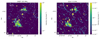 |
Fig. 4. GMRT 325 MHz (left) and JVLA 1.5 GHz C-configuration (right) radio maps of ZwCl 2341+0000, overlaid with contours at the 3σrms (solid) and −3σrms (dashed) levels. The beam sizes are plotted at the bottom-left corner of each image. Identified point sources that overlap with the southern relic are marked by red boxes. |
2.2.2. Spectral index map
Combining the GMRT image at 325 MHz and the JVLA C configuration image at 1.5 GHz we made a spectral index4 map of the cluster. We convolved the two images to the same Gaussian beam of 15.5 × 15.5 arcsec and excluded pixels below the respective 3σrms detection threshold in each image. In our case, the JVLA observation is shallower; therefore, we excluded the pixels in the convolved GMRT image to match the convolved JVLA image. The spectral index image was created using the CASA immath task with spix mode. The error map image was created propagating the rms noise of each image and the calibration error with the expression:
![$$ \begin{aligned} \sigma _\alpha =\frac{1}{\log \left(\nu _1/\nu _2\right)}\times \left[\sigma _{\rm sys}^2+\left(\frac{\sigma _{\nu _1}}{I_{\nu _1}}\right)^2+\left(\frac{\sigma _{\nu _2}}{I_{\nu _2}}\right)^2\right]^{1/2}, \end{aligned} $$](/articles/aa/full_html/2021/12/aa41540-21/aa41540-21-eq3.gif)
where ν1 and ν2 are the frequencies of the two images, σν is the rms noise of the image and Iν is the total intensity image at the frequency ν, and σsys is the calibration uncertainty, which is 5% here. The spectral index map between 325 MHz and 1.5 GHz is shown in Fig. 5.
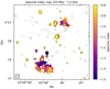 |
Fig. 5. Spectral index map between 325 MHz and 1.5 GHz with a resolution of 15.5″, overlaid with JVLA C-configuration contours. |
The spectral index at the SE edge of the radio relic RS-2 is −1.0. It steepens toward the cluster center down to −1.4. This is the first time the spectral steepening is resolved across the southern relic. However, the steepening in the relic RS-1 is less clear. Most of RS-1 has a flat spectral index of −0.9. The relic RN also shows spectral steepening, but with a gentle gradient. The spectral index decreases from −0.9 at the northern edge to −1.1 at the center.
We also computed a spectral index map between 325 MHz and 3.0 GHz, where the 3.0 GHz image was published by Benson et al. (2017). This map exhibits a similar spectral steepening trend as the spectral map between 325 MHz and 1.5 GHz, but with a lower spatial resolution.
3. Results
3.1. General X-ray properties
We fit a global spectrum in a circular region with radius r500, derived from the SZ mass (M500, SZ = 5.2 ± 0.4 M⊙, Planck Collaboration XXVII 2016), and centered at [23:43:42.1, +00:17:49.9], which is close to the pressure peak and the X-ray centroid (see the dashed circle in Fig. 2). We obtained kT = 5.32 ± 0.18 keV and Z = 0.29 ± 0.07 Z⊙, which are consistent with the results of previous Suzaku observation (Akamatsu & Kawahara 2013).
The previous shallow observation already shows that the X-ray emission is NW-SE elongated with substructures of an outbound bullet-like structure at the NW, a tail-like structure at the SE, and an excess emission toward the NE (Ogrean et al. 2014). The deep Chandra observations reveal new surface brightness features, which are marked in the top right panel of Fig. 1. The NE subcluster is actually a cone-shaped structure, where linear surface brightness edges are on the both sides of the cone. Below the cone, two wings stretch out toward the NE and SW directions, respectively. The apex of the cone is connected to the NE wing by a slim X-ray bridge. A linear surface brightness edge is in the SE direction, which was believed to be associated with the southern radio relic. In the SW direction, different from the SE linear structure, two surface brightness deficit regions are repeatedly shown.
Thermodynamic maps are plotted in Fig. 3. We also provide the temperature uncertainty map as in Fig. C.1. Limited by total counts and the size of the object, the spatial bins are coarse. Nevertheless, the thermodynamic maps still imply possible merging features, for example, shocks, cold fronts, and core remnants, for which we customize the surface brightness and spectral extraction regions for detailed investigation in the following subsections. In the temperature map, there are four regions where the temperatures are higher than the ambient regions, which are labeled as HT1–4. The region HT1 is close to the geometric center of the merging system, while HT1–3 are in relatively low density regions. HT2 is between the NW comet and NE wing, HT3 is outside the SE linear surface discontinuity, and HT4 is coincident with the two bays. In the pseudo pressure map, the pressure smoothly decreases from the HT1 to outer regions. There is no significant pressure jump across the inner edge of the HT2 and HT3 regions. There might be a sharp pressure gradient at the outer edge of the HT4 region and need to be further inspected. The entropy map shows three low entropy area, which correspond to the NW outbound cone (LK1), NE wing (LK2), and part of the SE linear structure (LK3). Because convection within clusters transfers low entropy gas to the bottom of gravitational potential wells and high entropy gas to the outskirts (e.g., Voit et al. 2002), low entropy gas is found in the cores of relaxed clusters. Therefore, the low entropy in those regions implies that the origin of the gas is related to cores of subclusters before the merger. The NW cone is a subcluster core being stripped. The SE linear structure is the remnant of a totally disrupted core, which is associated with the subcluster moving toward the SE.
3.2. SE edge
We extracted a 0.5−2.0 keV surface brightness profile across the SE linear structure using the region shown in the bottom panel of Fig. 1. The surface brightness profiles are plotted in the top left panel of Fig. 6. The surface brightness profile is similar to the profile in Fig. 3 of Ogrean et al. (2014), but with a factor of 2.4 higher signal to noise ratio. The deep observations reveal that the SE edge does not resemble other textbook examples of surface brightness discontinuities. The surface brightness profile is flat before a kink at ∼40″. After the kink, the surface brightness continuously decreases in a power law until a bump between the radii of 120″ and 160″. Although there is a significant change of the slope, there is no clear associated jump of density (see Markevitch & Vikhlinin 2007 for examples with sharp density jumps). The profile can be well fitted by a unprojected broken power law model with Cstat/d.o.f. = 35.4/38. The best-fit model was plotted as well. While using a single power law model, the fitting statistics is Cstat/d.o.f. = 179.2/40, which is much worse than using a broken power law, indicating an excess of X-ray emission contributed by a gas clump above the underlying density profile.
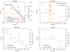 |
Fig. 6. Temperature and surface brightness (or emission measure) profiles in the SE edge, SW bays, NE wing, and western wing extraction regions. The region definitions are shown in the bottom panel of Fig. 1. |
Previous work on short observations was unable to explore temperature structures across the edge. With the deep observations, we tentatively search for potential temperature jumps. We plotted the temperature profile in the same panel as the surface brightness profile in Fig. 6. The temperature in the 0″ − 30″ and 30″ − 60″ bins are 4.6 ± 0.5 keV and 4.1 ± 0.5 keV, respectively, which are slightly below the averaged kT500 = 5.32 ± 0.18 keV. After that, it reaches  keV in the 60″ − 180″ bin. Outside this bin, the temperature cannot be constrained due to the fast decreasing surface brightness. Based on the temperature profile, there is no evidence for shock heating on the inner side of the kink, which disfavors the previous speculation by Ogrean et al. (2014) that the edge is a shock front. The existence of an additional gas clump as well as its relatively low temperature suggest that it is the remnant of the core of the southern subcluster, which agrees with the low entropy in the region LK3 (see Fig. 3). The high temperature outside the cool clump is likely to be heated by the leading shock. The pattern of a hot post shock region followed by a cool gas clump has been found in many post merger systems, where the cool component could be a remnant core either remains compact (e.g., Bullet Cluster, Markevitch et al. 2002; Markevitch 2006) or has been broken up (e.g., Abell 520, Wang et al. 2016). In our case, the core remnant is more diffuse, implying that either the progenitor is not a strong cool core or the diffusion processes has already taken place. We also estimated the 3σ lower limit of the temperature in 60″ − 180″ bin by using the ΔCstat = 9 criterion. The 3σ lower limit is 4.5 keV. We use this lower limit to constrain the Mach number of the undetected shock that is possible accelerating particles at the outer edge of the southern relic in Sect. 4.1.
The location of the shock front is unable to be resolved in X-rays due to the limited photons. Nevertheless, the functions of shocks in terms of particle acceleration shed light on the possible location. We plot the spectral index of the radio relic in the same panel. The radio relic has a relative flat spectrum at the outer edge (r ∼ 200″) and the spectral index decreases toward the cluster center. Based on the shock-relic connection established for most radio relics (e.g., Finoguenov et al. 2010), the position of the shock coincides with the flat edge, which is about 160″ (640 kpc) away from the cool gas clump.
3.3. SW bays
The locations of the two bays are coincident with a high temperature region in the temperature map (HT4). The gas outside this region has a lower temperature (< 4 keV). To locate the hot region in the NE-SW direction and search for possible temperature jumps, we extracted temperature profiles from the merging axis to the SW outskirts, the region configuration is defined in the bottom panel of Fig. 1. In addition, we extracted an emission measure profile that presents the trend of surface brightness (see the top right panel of Fig. 6). The third bin, ranging from 60″ to 90″ and covering most of the area of the two bays, has an extreme high temperature of  keV, which is a factor of
  higher than the second bin. After this bin, the temperature decreases to the average value of the cluster and reaches 3.4 ± 0.8 keV in the outermost bin.
The third temperature bin in the top right panel of Fig. 6 includes both bays. The profile in the NE-SW direction is unable to probe the origin of the hot gas and distinguish the thermodynamic properties of the individual bays. Therefore, we define perpendicular extraction regions along the NW-SE direction (see the top panel of Fig. 7). It starts from the western wing and goes through two bays and the remnant of the southern subcluster. The surface brightness and temperature profiles in the western slit region are shown in the bottom panel of Fig. 7. The temperature profile presents entirely different thermodynamic properties of the two bays. While the ICM in the northern bay is 3.3 ± 0.7 keV, the southern bay temperature is  keV. Furthermore, the ridge between the two bays has the highest temperature in the profile. Considering that the ridge has higher surface brightness than the two bays, which indicates a higher density, together with the high temperature, the gas in the two bays and the ridge does not hold pressure equilibrium. We measure the temperature by combining the two hot bins and obtain a
  keV temperature. Similar to the hot bin in the SE post shock region, we put a 3σ lower limit of 7.3 keV for this bin, which is still a factor of two higher than the temperature in the northern bay.
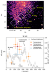 |
Fig. 7. Top: zoomed-in view of the western flank of the cluster. Individual temperature bins are plotted in white. The arrow indicates the direction of profiles. Bottom: temperature and surface brightness profiles extracted from the western slit region. |
3.4. NE and western wings
The temperature and emission measure profiles of the NE and western wing regions are plotted in the bottom left and bottom right panels of Fig. 6, respectively. The spectral extraction regions are designed to ensure at most 20% uncertainty for each temperature measurement. Therefore, we have six bins for the NE wing but only three bins for the western wing.
By visual inspection, we find no significant surface brightness jump across the NE wing, which is supported by the monotonously decreasing emission measure profile. However, the temperature profile exhibits features that are not seen in the surface brightness. The temperature in the innermost bin is 7.7 ± 1.2 keV, which is consistent with the HT1 region in the temperature map. Until r = 90″, the temperature drops monotonously, after which there is a sudden rise from 3.8 ± 0.5 keV to 6.1 ± 1.2 keV, where the jump has a significance of 1.8σ. This plausible temperature enhancement does not correspond to any surface brightness jump. After the jump, the temperature continuously decreases to 2.5 ± 0.5 keV at the wingtip.
On the contrary, the western wing does not show strong temperature variation, though the spatial bins are coarse due to the small size. The temperature at the wingtip is 4.7 ± 0.9 keV, which is closer to the averaged temperature of the cluster than the NE wingtip.
3.5. NW cone
The low entropy of the gas in the cone, the higher temperature of the ambient gas, and the equilibrium of the pressure across the cone show that this is an outbound subcluster core. Unlike any other observed remnant core cold front, this remnant core is not in a blunt-body shape, but in a cone shape. On both side of the cone, the cold fronts are linear and with projected lengths of ∼400 kpc. Unlike typical radial profiles, we extract a radially averaged surface brightness profile using sectors of annulus centered on the apex of the cone. The inner and outer radius are 50″ and 100″, respectively (see the bottom panel of Fig. 1). We define the azimuthal angle starting from the north and increasing eastward. The 2° binned profile is plotted in the top panel of Fig. 8. The bump centered at ∼85° is the “bridge” connecting the cone and the eastern wing. The surface brightness continuously increases from 100° to 115°. From 115°, which is the left edge of the cone, the surface brightness is relatively flat until a sudden drop at ∼150°. After the drop, the surface brightness is in a plateau for ∼15° then gradually fades away.
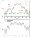 |
Fig. 8. Top: azimuthal surface brightness profile with a bin width of 2°. The vertical line is the axis of the cone. The 100° −136° and 136° −200° profiles are fitted separately. Bottom: zoomed-in view of the profile with a bin width of 1° together with the best-fit sigmoid model from 140° −170°. |
To probe the gas density inside the cone, we tentatively fit the profile using a projected broken power law model. The detailed description of the model and the projection of the conic body is in Appendix D. We first fit the entire profile from 100° to 200° to measure the width of the cone and the position angle of the axis. The center of the cone is at  and the gas density has a break at
  . However, a single component model cannot fit both sides of the conic subcluster well. The left side has a steeper gradient than the right side. Meanwhile, the best-fit power law index inside the cone α1 is negative, which indicates that the gas density at the edge is higher than the center. Therefore, we fit the 100° −136° and 136° −200° profiles separately. The parameter α1 is fixed to zero to investigate how much the observed profile deviates from a uniform gas distribution. The best-fit parameters of each profile are listed in Table 4. The left part can be well fitted with a uniform gas density in the cone. On the right part, the model cannot fit the profile at the jump well. The surface brightness enhancement before the jump indicates a high density shell at the cone edge.
Best-fit parameters of the surface brightness profiles across the cone.
We note that the surface brightness discontinuity on the right side of the axis is sharp. To further quantify the location of the jump, we binned the profile with a width of 1° (see the bottom panel of Fig. 8). The jump is at ∼154° in the 1° binned profile. On both sides of the jump, the profiles are flat. We tentatively fit the profile in the 140° −170° range to determine the jump location as well as the jump width using a sigmoid model. We adopted the form of error function, which is naturally a Gaussian convolved box function. In our case, the model is
where S0 and Sjump are profile normalization and jump strength, Φx the error function, θjump the jump location, and σ the width of the Gaussian smooth kernel. The best-fit jump location is  and the best-fit kernel width is
  .
.
3.6. Bridge and northern outskirts
We extracted the surface brightness profile across the bridge from the white narrow box region (the left half of the yellow broad region) in the top panel of Fig. 9. The surface brightness profile is plotted in the bottom panel of Fig. 9. The bridge is located at r ∼ 20″, after which the surface brightness keeps flat until a plausible jump at r ∼ 100″. To check the significance of the bridge and the jump, we fit the profile using a compound model that consists of a Gaussian profile and a projected double power law density profile. The best-fit surface brightness of the Gaussian component is (9.1 ± 3.0)×10−6 cts s−1 cm−2 arcmin−2, which means that the gas bridge has a 3σ detection. The best-fit density jump is 1.6 ± 0.6, which is unconstrained due to the limit of counts. However, the best-fit power law index changes from 0.0 ± 0.1 before the jump to  after the jump. We extracted a surface brightness profile using a broad region (the yellow box in the top panel of Fig. 9) to check whether the potential jump is associated with the northern relic. The surface brightness in the broad region is plotted in the bottom panel of Fig. 9 as well. The profile has a similar trend as that in the narrow region and the best-fit jump location is 108″ ± 4, which is close to the outer edge of the northern relic. The best-fit density jump of the broad region profile is 1.8 ± 1.1, which means that the density jump still cannot be constrained.
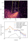 |
Fig. 9. Top: narrow (white) and broad (yellow) extraction regions for surface brightness profiles in the northern outskirts. The dashed contour is the northern relic in the GMRT 325 MHz image at the 3σrms level. Bottom: surface brightness profiles and their best-fit model in the narrow and broad regions. The bridge and the surface brightness jump are located at r = 23″ and r = 108″, respectively. The GMRT 325 MHz profile is plotted with a dashed curve, the outer edge of which is associated with the potential X-ray jump. |
4. Discussion
4.1. Shock fronts and radio relics
By measuring the temperature profile, we discovered that the previous SE surface brightness jump reported by Ogrean et al. (2014) is not a shock but rather a kink contributed by cool gas from the remnant core. Outside the kink, the X-ray surface brightness drops dramatically, preventing us from investigating the exact location of the shock in the X-rays. Nevertheless, at radio frequencies, the 325 MHz−1.5 GHz spectral index map clearly shows the spectral steepening from the edge toward the cluster center. It is the first time that we see the evidence of shock acceleration and subsequent radiative cooling of the relativistic plasma in the radio relic of this cluster. The spectrally flat edge of the southern relic, which is ∼160″ away from the kink, is the possible location of the southern shock.
In the northern relic, the spectral index is flat at the northern edge, where the X-ray surface brightness changes its gradient. Although the density jump cannot be constrained, the variation in the gradient at this position suggests that the northern shock that is responsible for (re)accelerating the northern relic is at this position.
Based on the DSA theory, the radio injection spectral index is a function of the Mach number,
Since the spectral index is spatially resolved, this relation can be directly applied to the southern relic, where the injection spectral index is 1.00 ± 0.06. We obtain a radio Mach number ℳradio, S = 2.2 ± 0.1. This number is lower than using the integrated spectral index αS, int = −1.20 ± 0.18 (Benson et al. 2017) and assuming the relation between the injection and integrated spectral indices is αint = αinj − 0.5 (Kardashev 1962). A theoretical investigation shows that this simple assumption does not hold when the shock is nonstationary, which is the case of cluster merger shocks (Kang 2015). We also applied Eq. (3) to the northern relic. The updated radio Mach number ℳradio, N = 2.4 ± 0.4.
Meanwhile, the Mach number can be estimated by using the temperature jump based on the Rankine-Hugoniot condition (Landau & Lifshitz 1959),
The pre-shock region is too faint to measure the temperature. Therefore, we tentatively extrapolate it by using a universal temperature profile (Burns et al. 2010), which remarkably agrees with Suzaku observations of galaxy cluster outskirts. The profile is
![$$ \begin{aligned} \frac{kT(r)}{kT_{\rm ave}}=(1.74\pm 0.03)\times \left[1+(0.64\pm 0.10)\times \left(\frac{r}{r_{200}}\right)\right]^{-3.2\pm 0.4}. \end{aligned} $$](/articles/aa/full_html/2021/12/aa41540-21/aa41540-21-eq22.gif)
The spectrally flat boundary of the relic is located at r ∼ 0.7 r200, at which the predicted pre-shock temperature is 2.8 ± 0.6 keV. Because the temperature measurement in the post shock region has a large error bar, we only put a lower limit for that Mach number. By combining the 3σ lower limit of the post-shock temperature 4.5 keV, we obtain the 3σ lower limit of the X-ray Mach number 1.6. The estimated lower limit of the X-ray Mach number matches the value of the radio Mach number. Because we can only put a lower limit of the X-ray Mach number, it is not clear whether this shock is another case with Mach number discrepancy between the X-ray and the radio. Unfortunately, in the X-ray, the temperature between the bridge and the potential jump in the northern outskirts (see Fig. 9) is not constrained.
4.2. Conic subcluster
The shapes of the subclusters in other merging systems usually show a spheroid core, and the surface brightness decreases radially from the center of the core. As an exception, the subcluster in ZwCl 2341+0000 does not have a concentrated surface brightness peak and the radius of curvature at the apex can be limited to be less than 30 kpc. As a comparison, the straight cold fronts on both sides have lengths of 400 kpc. Meanwhile, by using a surface brightness profile fit, we estimated that the gas density at the center of the cone is about 10−3 cm−3, which is relatively low among all cool core and non cool core clusters (e.g., Hudson et al. 2010). The corresponding cooling time is about 27 Gyr, which is much larger than the Hubble time, implying an expansion of the core after the collision with another subcluster.
An analogy of the cone-shaped subcluster in simulations is presented in Fig. 9 of Zhang et al. (2019) at t = 0.03 Gyr. As a bullet-like subcluster leaves the atmosphere of the main cluster, due to the decrease in pressure, the far end starts to expand while the two sides are still under ram pressure stripping. Thus, the bullet-like subcluster is elongated and deformed. A cone-shaped subcluster with a narrow aperture appears at a certain stage of the merging process. We note that in ZwCl 2341+0000, the projected brightest cluster galaxy position is outside but very close to the apex of the cone, indicating that the dark matter sub-halo is still leading the gaseous subcluster. As the merger goes on, the tip of the cone will be continuously expanding to form a slingshot cold front (e.g., Abell 168 Hallman & Markevitch 2004). Another similar analogy is the R = 1 : 3 and b = 0 kpc simulation set in ZuHone (2011)5. At t = 1.6 Gyr, the subcluster evolves to be a cone with an aperture of 40°, which is similar with the observed conic structure. The fate of the conic subcluster in this simulation is the same as the one in Zhang et al. (2019). After this epoch, the tip of the cone starts to expand in the low density outskirts. This simulation also produces a dense gas shell at the cone boundary, which is similar to the right part of the cone in ZwCl 2341+0000.
4.2.1. Effect of magnetic fields
During a merger, the magnetic field in the cluster can be amplified through multiple processes and could produce observable features such as plasma depletion layers (see Donnert et al. 2018, for a review). We investigate the effect of magnetic field in forming such conic subclusters by comparing a pure hydrodynamic (HD) simulation and a magnetohydrodynamic (MHD) simulation. With the same merger configurations as ZuHone (2011), Brzycki & ZuHone (2019) carried out MHD simulations with initial condition β = 2006. Similarly, we ran a new MHD simulation of the 1 : 3 mass ratio with β = 100, where the effect of magnetic field should be more significant than the β = 200 simulation. We created mock images by putting both the HD and MHD simulations at z = 0.27 with ACIS configuration and 200 ks exposure time. The mock image of the MHD simulation is shown in the top panel of Fig. 10.
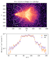 |
Fig. 10. Top: mock X-ray image of a cone-shaped subcluster in the β = 100 MHD simulation, whose merger configuration is the same as in ZuHone (2011) and Brzycki & ZuHone (2019). In this snapshot, two wing-like structures in addition to the cone are reproduced as well. Bottom: azimuthal surface brightness profiles extracted from the mock observations of the MHD (orange) and HD (purple) simulations. |
We extracted azimuthal surface brightness profiles for the simulated conic subclusters. The profiles are plotted in the bottom panel of Fig. 10. The MHD simulation has a similar profile as the pure HD simulation, which means that the magnetic field with a β = 100 initial condition does not play a significant role in shaping the conic subcluster. Moreover, we do not find significant plasma depletion layers that push gas out and exhibit dark streaks in the image (as was found by, e.g., Werner et al. 2016 in a deep observation of the Virgo sloshing cold front). Therefore, the observed conic structure is consistent with both HD and MHD simulations and the effect of magnetic fields cannot yet be ascertained with the current data.
4.2.2. Gas bridge and ICM viscosity
In addition to the rare conic subcluster, the X-ray bridge structure is seldom discovered. The temperature of the bridge itself is 4.3 ± 1.1 keV and that of the combination of the bridge and the dark pocket below the bridge is 8.6 ± 2.4 keV. The similar temperature of the bridge and the cone indicates that the bridge could be the stripped gas trail from the cone. A similar structure has been found in M 89, where two horns are attached to the front of the remnant core (Machacek et al. 2006). Kraft et al. (2017) argues that the horns could either be Kelvin-Helmholtz instability (KHI) eddies with a viewing angle of 30° or be due to the previous active galactic nucleus activities. Another similar case is galaxy group UGC 12491 (Roediger et al. 2012), where the stripped tails split from the core. Although our cluster has an order of magnitude larger physical scale than the cases of M 89 and UGC 12491, because HD is scale-free, the KHI could still be responsible for the stripped gas trail in our system. If this gas trail is from a KHI eddy, based on its 400 kpc length, it should be stripped at the time when the stagnation point of the subcluster was about 400 kpc closer to the system centroid, and then evolves together with the subcluster.
Viscosity suppresses the development of KHI eddies that are smaller than a critical scale. In turn, with the existence of an eddy at a certain scale, we are able to constrain the upper limit of the viscosity μ, whose expression is given by Ichinohe et al. (2021):
where nout is the ICM density outside the cold front, λ the scale of the eddy, V the shear velocity, a a coefficient to be 10 for a conservative estimation, Δ ≡ (ρ1 + ρ2)2/(ρ1ρ2) calculated using the gas densities inside and outside the cold front. In our case, nout ∼ 5 × 10⁻⁴ cm−3, which is about a factor of three lower than that in the cone. The scale of eddy is 400 kpc. We take the collision speed at pericenter 1900 km s−1 (Benson et al. 2017) to be an upper limit of the shear velocity. We obtain an upper limit of viscosity of ∼5000 g cm−1 s−1. The full isotropic Spitzer viscosity is
assuming Coulomb logarithm lnΛ = 40 (Spitzer 1956; Sarazin 1988). A ∼9 keV ICM has μSP ∼ 6200 g cm−1 s−1, which means the viscosity is suppressed at least by a factor of 1.2 if the gas trail has a KHI origin. With only this long gas trail, we cannot place strict constraints on the viscosity suppression factor, which is at least three in other systems, for example, three for Abell 2319 (Ichinohe et al. 2021), five for Abell 2142 (Wang & Markevitch 2018), and 20 for Abell 3667 (Ichinohe et al. 2017).
4.2.3. Suppression of diffusion
We note that the western side of the cone has a sharp surface brightness jump, whose width has 1σ upper limit of 2.4° azimuth. Though this cluster has a relatively high redshift of 0.27, at which the projected linear scale corresponding to a 2.4° bin at the radius of 100″ is 17 kpc, it is still worthwhile to inspect whether the diffusion is suppressed to form the observed sharp edge. Assuming the ICM is in thermal equilibrium, the mean free path of electrons is given by Sarazin (1988),
The mean free path is about 4.1 kpc for a kT = 4.5 keV and ne = 1.5 × 10⁻³ cm−3 ICM inside the cold front, and is about 13.1 kpc for a kT = 6.5 keV and ne = 1 × 10⁻³ cm−3 ICM outside the cold front. Meanwhile, the mean free path of the particles moving from one side of the cold front to the other side is given by Vikhlinin et al. (2001),
where G(x) = [Φ(x)−xΦ′(x)]/2x2 and Φ(x) is the error function, the subscripts A and B represent inside and outside of the cold front, and vice versa. The mean free path for particles moving from inside to the outside is λin → out = 9.2 kpc. The unsuppressed Coulomb diffusion will smear the density discontinuity by several mean free paths, which is comparable with the 1σ upper limit of the projected jump width. Therefore, without future deeper high spatial resolution observations, we cannot draw a solid conclusion whether the diffusion is suppressed.
4.3. The origin of the NE wing
In some head-on mergers, gas plumes perpendicular to the merging axis are observed, for example Abell 168 (Hallman & Markevitch 2004), Abell 2146 (Russell et al. 2010, 2012). Russell et al. (2012) suggest that the structure in Abell 2146 is likely to be part of the remnant core of the primary subcluster, which was pushed forward and laterally by the collision. This scenario can also be applied to this merging system where we observe two wings behind the outbound NW subcluster.
However, the size of NE wing is considerable and is even larger than the NW conic subcluster. Thus, it may have a different origin. The optical analysis suggests that in addition to the z = 0.2687 northern subcluster that is associated with the cone in X-ray and the z = 0.2684 southern subcluster that is associated with the southern linear structure, a third subcluster at z = 0.2743 is spatially overlaid with the northern subcluster (Benson et al. 2017). The large NE wing may belong to the third subcluster and was displaced to the NE direction. To prove this scenario, we search for galaxies that around the NE wing tip in the redshift catalog of Benson et al. (2017). We find several galaxies there, but all of them are at z ∼ 0.270. If the NE wing is associated with those galaxies, it is more likely to be from the either the z = 0.2687 northern subcluster or the z = 0.2684 southern subcluster.
Therefore, we prefer the scenario of a displaced gas clump due to the head-on collision. The mystery of the remarkable size of the NE wing needs to be further investigated by numerical simulations with specific merging parameters.
5. Conclusion
We analyzed the deep Chandra observations of merging galaxy cluster ZwCl 2341+0000. The cluster is elongated in the NW-SE direction. Meanwhile, we used GMRT and JVLA data to investigate the properties of the radio shocks. We summarize the main results as follows:
-
The SE linear surface brightness edge is a kink in the new observations. It is the disrupted core of the southern subcluster. The shock front that is possibly responsible for the southern radio relic is revealed by the radio spectral index maps and is located at the SE edge of the relic component S2, which is ∼160″ (640 kpc) away from the SE surface brightness kink.
-
At radio wavelengths, the Mach numbers of the southern and northern shocks are 2.2 ± 0.1 and 2.4 ± 0.4, based on injection spectral indices and the assumption of DSA. In X-rays, assuming the pre-shock ICM temperature follows a universal profile of relaxed clusters, we obtain a 3σ lower limit of the southern shock Mach number of 1.6.
-
The NW subcluster has a cone shape with two linear ∼400 kpc cold fronts on the two sides. We searched for analogies of the cone-shaped subcluster in numerical simulations and found that the cone is a certain stage of an outbound subcluster in the head-on merger, which happens between a bullet-like morphology and a slingshot phase. This stage is short-lived, and no other example has been discovered to date.
-
Behind the NW conic subcluster, there are two wing structures stretching out in the NE and western directions. The NE wing is broad and has a low temperature and entropy at the tip. The redshift of galaxies around the wingtip suggests that this structure is unlikely to be associated with the third subcluster discovered in the previous optical analysis. This may thus represent an unexpectedly large gas plume expanding perpendicular to the merger axis.
-
A 400 kpc cool (∼4 keV) gas bridge connects the apex of the NW cone and the NE wing. The low temperature suggests that this is a stripped gas trail from the NW subcluster. Why it is split from the subcluster is unclear. It could have evolved from a KHI eddy.
-
There are two surface brightness bays located in the SW periphery. The southern bay and the ridge between the two bays have a > 10 keV temperature, while the northern bay has a 3.3 ± 0.7 keV temperature. There is no pressure equilibrium between the ridge and the northern bay. The physical origin of these features is still unclear.
In summary, ZwCl 2341+0000 is an exciting galaxy cluster merger that exhibits several unique morphology features. It is likely in a short-lived phase that is rarely observed and offers an example of the complex transition between a bullet-like morphology and the development of a slingshot tail.
Acknowledgments
We thank the anonymous referee for useful comments and suggestions that helped improve this paper. X.Z. acknowledges support from Chinese Scholarship Council (CSC). A.S. is supported by the Women In Science Excel (WISE) programme of the Netherlands Organisation for Scientific Research (NWO), and acknowledges the World Premier Research Center Initiative (WPI) and the Kavli IPMU for the continued hospitality. SRON Netherlands Institute for Space Research is supported financially by NWO. R.J.vW. acknowledges support from the ERC Starting Grant ClusterWeb 804208. C.S. and A.B. acknowledge support from ERC-Stg DRANOEL n. 714245. This research has made use of data obtained from the Chandra Data Archive and the Chandra Source Catalog, and software provided by the Chandra X-ray Center (CXC) in the application package CIAO. The National Radio Astronomy Observatory is a facility of the National Science Foundation operated under cooperative agreement by Associated Universities, Inc. We thank the staff of the GMRT who have made these observations possible. The GMRT is run by the National Centre for Radio Astrophysics of the Tata Institute of Fundamental Research. This work made use of data from the Galaxy Cluster Merger Catalog. This research made use of Astropy (http://www.astropy.org), a community-developed core Python package for Astronomy (Astropy Collaboration 2013, 2018).
References
- Akamatsu, H., & Kawahara, H. 2013, PASJ, 65, 16 [NASA ADS] [CrossRef] [Google Scholar]
- Ascasibar, Y., & Markevitch, M. 2006, ApJ, 650, 102 [Google Scholar]
- Astropy Collaboration (Robitaille, T. P., et al.) 2013, A&A, 558, A33 [NASA ADS] [CrossRef] [EDP Sciences] [Google Scholar]
- Astropy Collaboration (Price-Whelan, A. M., et al.) 2018, AJ, 156, 123 [Google Scholar]
- Bagchi, J., Enßlin, T. A., Miniati, F., et al. 2002, New Astron., 7, 249 [NASA ADS] [CrossRef] [Google Scholar]
- Bell, A. R. 1978, MNRAS, 182, 147 [Google Scholar]
- Benson, B., Wittman, D. M., Golovich, N., et al. 2017, ApJ, 841, 7 [NASA ADS] [CrossRef] [Google Scholar]
- Blandford, R. D., & Ostriker, J. P. 1978, ApJ, 221, L29 [Google Scholar]
- Boschin, W., Girardi, M., & Barrena, R. 2013, MNRAS, 434, 772 [NASA ADS] [CrossRef] [Google Scholar]
- Botteon, A., Gastaldello, F., & Brunetti, G. 2018, MNRAS, 476, 5591 [Google Scholar]
- Brzycki, B., & ZuHone, J. 2019, ApJ, 883, 118 [NASA ADS] [CrossRef] [Google Scholar]
- Burns, J. O., Skillman, S. W., & O’Shea, B. W. 2010, ApJ, 721, 1105 [NASA ADS] [CrossRef] [Google Scholar]
- Cash, W. 1979, ApJ, 228, 939 [Google Scholar]
- Cornwell, T. J., Golap, K., & Bhatnagar, S. 2008, IEEE J. Sel. Top. Signal Process., 2, 647 [Google Scholar]
- de Plaa, J. 2020, https://doi.org/10.5281/zenodo.3707693 [Google Scholar]
- Dominguez-Fernandez, P., Bruggen, M., Vazza, F., et al. 2021, MNRAS, 500, 795 [Google Scholar]
- Donnert, J., Vazza, F., Brüggen, M., & ZuHone, J. 2018, Space Sci. Rev., 214, 122 [Google Scholar]
- Finoguenov, A., Sarazin, C. L., Nakazawa, K., Wik, D. R., & Clarke, T. E. 2010, ApJ, 715, 1143 [Google Scholar]
- Fruscione, A., McDowell, J. C., Allen, G. E., et al. 2006, in Society of Photo-Optical Instrumentation Engineers (SPIE) Conference Series, eds. D. R. Silva, & R. E. Doxsey, 6270, 62701V [NASA ADS] [Google Scholar]
- Ghizzardi, S., Rossetti, M., & Molendi, S. 2010, A&A, 516, A32 [NASA ADS] [CrossRef] [EDP Sciences] [Google Scholar]
- Giovannini, G., Bonafede, A., Feretti, L., Govoni, F., & Murgia, M. 2010, A&A, 511, L5 [NASA ADS] [CrossRef] [EDP Sciences] [Google Scholar]
- Gunn, J. E., & Gott, J. R., III 1972, ApJ, 176, 1 [Google Scholar]
- Hallman, E. J., & Markevitch, M. 2004, ApJ, 610, L81 [Google Scholar]
- Hong, S. E., Kang, H., & Ryu, D. 2015, ApJ, 812, 49 [NASA ADS] [CrossRef] [Google Scholar]
- Hudson, D. S., Mittal, R., Reiprich, T. H., et al. 2010, A&A, 513, A37 [NASA ADS] [CrossRef] [EDP Sciences] [Google Scholar]
- Ichinohe, Y., Simionescu, A., Werner, N., & Takahashi, T. 2017, MNRAS, 467, 3662 [Google Scholar]
- Ichinohe, Y., Simionescu, A., Werner, N., Markevitch, M., & Wang, Q. H. S. 2021, MNRAS, 504, 2800 [CrossRef] [Google Scholar]
- Intema, H. T. 2014, Astron. Soc. India Conf. Ser., 13, 469 [Google Scholar]
- Intema, H. T., van der Tol, S., Cotton, W. D., et al. 2009, A&A, 501, 1185 [NASA ADS] [CrossRef] [EDP Sciences] [Google Scholar]
- Kaastra, J. S. 2017, A&A, 605, A51 [NASA ADS] [CrossRef] [EDP Sciences] [Google Scholar]
- Kaastra, J. S., & Bleeker, J. A. M. 2016, A&A, 587, A151 [NASA ADS] [CrossRef] [EDP Sciences] [Google Scholar]
- Kaastra, J. S., Mewe, R., & Nieuwenhuijzen, H. 1996, UV and X-ray Spectroscopy of Astrophysical and Laboratory Plasmas, 411 [Google Scholar]
- Kaastra, J. S., Raassen, A. J. J., de Plaa, J., & Gu, L. 2020, https://doi.org/10.5281/zenodo.3939056 [Google Scholar]
- Kang, H. 2015, J. Korean Astron. Soc., 48, 9 [Google Scholar]
- Kardashev, N. S. 1962, Sov. Astron., 6, 317 [NASA ADS] [Google Scholar]
- Kraft, R. P., Roediger, E., Machacek, M., et al. 2017, ApJ, 848, 27 [NASA ADS] [CrossRef] [Google Scholar]
- Krymskii, G. F. 1977, Akademiia Nauk SSSR Doklady, 234, 1306 [NASA ADS] [Google Scholar]
- Kuntz, K. D., & Snowden, S. L. 2000, ApJ, 543, 195 [Google Scholar]
- Landau, L. D., & Lifshitz, E. M. 1959, Fluid Mechanics (London: Pergamon Press) [Google Scholar]
- Lehmer, B. D., Xue, Y. Q., Brandt, W. N., et al. 2012, ApJ, 752, 46 [NASA ADS] [CrossRef] [Google Scholar]
- Lodders, K., Palme, H., & Gail, H.-P. 2009, 4.4 Abundances of the Elements in the Solar System: Datasheet from Landolt-Börnstein– Group VI Astronomy and Astrophysics (Berlin, Heidelberg: Springer-Verlag) [Google Scholar]
- Machacek, M., Jones, C., Forman, W. R., & Nulsen, P. 2006, ApJ, 644, 155 [NASA ADS] [CrossRef] [Google Scholar]
- Markevitch, M. 2006, in The X-ray Universe 2005, ed. A. Wilson, ESA Spec. Publ., 604, 723 [NASA ADS] [Google Scholar]
- Markevitch, M., & Vikhlinin, A. 2007, Phys. Rep., 443, 1 [Google Scholar]
- Markevitch, M., Gonzalez, A. H., David, L., et al. 2002, ApJ, 567, L27 [Google Scholar]
- Ogrean, G. A., Brüggen, M., van Weeren, R. J., Burgmeier, A., & Simionescu, A. 2014, MNRAS, 443, 2463 [CrossRef] [Google Scholar]
- Owers, M. S., Nulsen, P. E. J., Couch, W. J., & Markevitch, M. 2009, ApJ, 704, 1349 [Google Scholar]
- Perley, R. A., & Butler, B. J. 2013, ApJS, 204, 19 [Google Scholar]
- Planck Collaboration XXVII. 2016, A&A, 594, A27 [NASA ADS] [CrossRef] [EDP Sciences] [Google Scholar]
- Rau, U., & Cornwell, T. J. 2011, A&A, 532, A71 [NASA ADS] [CrossRef] [EDP Sciences] [Google Scholar]
- Roediger, E., Kraft, R. P., Machacek, M. E., et al. 2012, ApJ, 754, 147 [NASA ADS] [CrossRef] [Google Scholar]
- Russell, H. R., Sanders, J. S., Fabian, A. C., et al. 2010, MNRAS, 406, 1721 [Google Scholar]
- Russell, H. R., McNamara, B. R., Sanders, J. S., et al. 2012, MNRAS, 423, 236 [NASA ADS] [CrossRef] [Google Scholar]
- Sabol, E. J., & Snowden, S. L. 2019, Astrophysics Source Code Library [record ascl:1904.001] [Google Scholar]
- Sanders, J. S. 2006, MNRAS, 371, 829 [Google Scholar]
- Sarazin, C. L. 1988, X-ray Emission from Clusters of Galaxies (Cambridge: Cambridge University Press) [Google Scholar]
- Spitzer, L. 1956, Physics of Fully Ionized Gases (New York: Interscience Publishers) [Google Scholar]
- Tittley, E. R., & Henriksen, M. 2005, ApJ, 618, 227 [Google Scholar]
- van Weeren, R. J., Röttgering, H. J. A., Bagchi, J., et al. 2009, A&A, 506, 1083 [NASA ADS] [CrossRef] [EDP Sciences] [Google Scholar]
- van Weeren, R. J., Ogrean, G. A., Jones, C., et al. 2016, ApJ, 817, 98 [Google Scholar]
- van Weeren, R. J., de Gasperin, F., Akamatsu, H., et al. 2019, Space Sci. Rev., 215, 16 [Google Scholar]
- Vikhlinin, A., Markevitch, M., & Murray, S. S. 2001, ApJ, 551, 160 [NASA ADS] [CrossRef] [Google Scholar]
- Voit, G. M., Bryan, G. L., Balogh, M. L., & Bower, R. G. 2002, ApJ, 576, 601 [NASA ADS] [CrossRef] [Google Scholar]
- Wang, Q. H. S., & Markevitch, M. 2018, ApJ, 868, 45 [CrossRef] [Google Scholar]
- Wang, Q. H. S., Markevitch, M., & Giacintucci, S. 2016, ApJ, 833, 99 [NASA ADS] [CrossRef] [Google Scholar]
- Werner, N., ZuHone, J. A., Zhuravleva, I., et al. 2016, MNRAS, 455, 846 [NASA ADS] [CrossRef] [Google Scholar]
- Willingale, R., Starling, R. L. C., Beardmore, A. P., Tanvir, N. R., & O’Brien, P. T. 2013, MNRAS, 431, 394 [Google Scholar]
- Zhang, X. 2021, https://doi.org/10.5281/zenodo.5507575 [Google Scholar]
- Zhang, C., Churazov, E., Forman, W. R., & Jones, C. 2019, MNRAS, 482, 20 [NASA ADS] [CrossRef] [Google Scholar]
- Zhang, X., Simionescu, A., Akamatsu, H., et al. 2020, A&A, 642, A89 [NASA ADS] [CrossRef] [EDP Sciences] [Google Scholar]
- ZuHone, J. A. 2011, ApJ, 728, 54 [Google Scholar]
- Zuhone, J. A., & Roediger, E. 2016, J. Plasma Phys., 82, 535820301 [CrossRef] [Google Scholar]
Appendix A: JVLA B-configuration radio map
The JVLA L-band B-configuration image is plotted in Fig. A.1, where most of the relics are not visible.
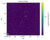 |
Fig. A.1. JVLA 1.5 GHz B-configuration radio map of ZwCl 2341+0000. |
Appendix B: Radio spectral index uncertainty map
The spectral index uncertainty map between 325 MHz and 1.5 GHz is plotted in Fig. B.1. We also plot the spectral index map between 325 MHz and 3.0 GHz as well as its uncertainty map.
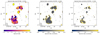 |
Fig. B.1. Left and Middle: Spectral index map and the uncertainty between 325 MHz and 3.0 GHz. Right: Spectral index uncertainty map between 325 MHz and 1.5 GHz. |
Appendix C: Temperature uncertainty map
The uncertainties of the pseudo pressure and entropy are dominated by the uncertainty of the temperature. The temperature uncertainty map (Fig. C.1) shows that most regions of interests have an uncertainty less than 20%. Only the region HT3 has an uncertainty about 35%.
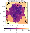 |
Fig. C.1. Temperature uncertainty map of ZwCl 2341+0000 in units of percent, overlaid with the X-ray surface brightness contours. |
Appendix D: Projected surface brightness profile for a cone-shaped cold front
We assume the core remnant is in a right circular cone shape. For a given point in the space, the electron density can be expressed as a function of the distance to the apex ρ and the angle with respect to the cone axis ϕ (i.e., ne = ne(ρ,ϕ)). Similar to the broken power law model applied on a spheroid (Owers et al. 2009), we define a broken power law density profile across a cone-shaped cold front,
where n0 is the electron density normalization, ϕb the angle of the discontinuity, C the density jump, α1 and α2 the power law index inside and outside the discontinuity, the term (ρ/ρ0)−αρ is the density variation along the axis, which is approximately negligible since the radial surface brightness is averaged. We assume the gas density is zero where ϕ > ϕmax.
The cone is projected to the plane of the sky. Assuming the axis is parallel to the sky plane, the integrated surface brightness at any point of the sky plane (r, θ) is
where lmax = r × [1−(cos ϕmax/cos θ)2]1/2 is the boundary of the integration. Therefore, the radially averaged surface brightness is
where rmin and rmax are the inner and outer radii of the extraction sector.
All Tables
X-ray foreground and background components constrained by the RASS and Chandra offset spectra.
All Figures
|
Fig. 1. Top left: X-ray flux map in the 0.5−2.0 keV band convolved with a σ = 1.97″ (four pixel) Gaussian kernel. Overlaid are the JVLA C-array 1.5 GHz radio contours at [1, 2, 4]×0.075 mJy beam−1. The terms of the relic sources RS-1–3 and RN are introduced by van Weeren et al. (2009). Identified point sources that overlap with the southern relic are marked by cyan boxes. Top right: image from which point sources have been removed. Surface brightness features are labeled. The locations of the three brightest cluster galaxies adopted from Benson et al. (2017) are marked as cyan crosses. Bottom: extraction regions used for detailed X-ray analysis in Sect. 3. For the regions SE edge, SW bays, western wing, and NE wing, the individual temperature bins in Fig. 6 are plotted. The arrows beside each bin indicate the directions of the profiles. |
| In the text | |
|
Fig. 2. Illustration of the offset extraction region, which is the white rectangle. Point-like sources are excluded using red regions, including the red rectangle, which is used to collectively exclude a series of observed clumps. The dashed circle is the r500 region of the cluster, which is centered at [23:43:42.1, +00:17:49.9]. |
| In the text | |
|
Fig. 3. Temperature, pseudo pressure, and entropy maps of ZwCl 2341+0000, overlaid with the X-ray surface brightness contours. High temperature and low entropy regions are labeled as HT1–4 and LK1–3, respectively. |
| In the text | |
|
Fig. 4. GMRT 325 MHz (left) and JVLA 1.5 GHz C-configuration (right) radio maps of ZwCl 2341+0000, overlaid with contours at the 3σrms (solid) and −3σrms (dashed) levels. The beam sizes are plotted at the bottom-left corner of each image. Identified point sources that overlap with the southern relic are marked by red boxes. |
| In the text | |
|
Fig. 5. Spectral index map between 325 MHz and 1.5 GHz with a resolution of 15.5″, overlaid with JVLA C-configuration contours. |
| In the text | |
|
Fig. 6. Temperature and surface brightness (or emission measure) profiles in the SE edge, SW bays, NE wing, and western wing extraction regions. The region definitions are shown in the bottom panel of Fig. 1. |
| In the text | |
|
Fig. 7. Top: zoomed-in view of the western flank of the cluster. Individual temperature bins are plotted in white. The arrow indicates the direction of profiles. Bottom: temperature and surface brightness profiles extracted from the western slit region. |
| In the text | |
|
Fig. 8. Top: azimuthal surface brightness profile with a bin width of 2°. The vertical line is the axis of the cone. The 100° −136° and 136° −200° profiles are fitted separately. Bottom: zoomed-in view of the profile with a bin width of 1° together with the best-fit sigmoid model from 140° −170°. |
| In the text | |
|
Fig. 9. Top: narrow (white) and broad (yellow) extraction regions for surface brightness profiles in the northern outskirts. The dashed contour is the northern relic in the GMRT 325 MHz image at the 3σrms level. Bottom: surface brightness profiles and their best-fit model in the narrow and broad regions. The bridge and the surface brightness jump are located at r = 23″ and r = 108″, respectively. The GMRT 325 MHz profile is plotted with a dashed curve, the outer edge of which is associated with the potential X-ray jump. |
| In the text | |
|
Fig. 10. Top: mock X-ray image of a cone-shaped subcluster in the β = 100 MHD simulation, whose merger configuration is the same as in ZuHone (2011) and Brzycki & ZuHone (2019). In this snapshot, two wing-like structures in addition to the cone are reproduced as well. Bottom: azimuthal surface brightness profiles extracted from the mock observations of the MHD (orange) and HD (purple) simulations. |
| In the text | |
|
Fig. A.1. JVLA 1.5 GHz B-configuration radio map of ZwCl 2341+0000. |
| In the text | |
|
Fig. B.1. Left and Middle: Spectral index map and the uncertainty between 325 MHz and 3.0 GHz. Right: Spectral index uncertainty map between 325 MHz and 1.5 GHz. |
| In the text | |
|
Fig. C.1. Temperature uncertainty map of ZwCl 2341+0000 in units of percent, overlaid with the X-ray surface brightness contours. |
| In the text | |
Current usage metrics show cumulative count of Article Views (full-text article views including HTML views, PDF and ePub downloads, according to the available data) and Abstracts Views on Vision4Press platform.
Data correspond to usage on the plateform after 2015. The current usage metrics is available 48-96 hours after online publication and is updated daily on week days.
Initial download of the metrics may take a while.