| Issue |
A&A
Volume 656, December 2021
|
|
|---|---|---|
| Article Number | A99 | |
| Number of page(s) | 20 | |
| Section | Cosmology (including clusters of galaxies) | |
| DOI | https://doi.org/10.1051/0004-6361/202141521 | |
| Published online | 08 December 2021 | |
Cosmology with the submillimetre galaxies magnification bias
Tomographic analysis⋆
1
Departamento de Fisica, Universidad de Oviedo, C. Federico Garcia Lorca 18, 33007 Oviedo, Spain
e-mail: This email address is being protected from spambots. You need JavaScript enabled to view it.
2
Instituto Universitario de Ciencias y Tecnologías Espaciales de Asturias (ICTEA), C. Independencia 13, 33004 Oviedo, Spain
3
International School for Advanced Studies (SISSA), via Bonomea 265, 34136 Trieste, Italy
4
INFN Sezione di Trieste, via Valerio 2, 34127 Trieste, Italy
5
Institute for Fundamental Physics of the Universe (IFPU), Via Beirut 2, 34014 Trieste, Italy
6
Dipartimento di Fisica, Università di Roma Tor Vergata, Via della Ricerca Scientifica, 1, Roma, Italy
7
INFN, Sezione di Roma 2, Università di Roma Tor Vergata, Via della Ricerca Scientifica, 1, Roma, Italy
Received:
11
June
2021
Accepted:
15
September
2021
Abstract
Context. High-z submillimetre galaxies can be used as a background sample for gravitational lensing studies thanks to their magnification bias. In particular, the magnification bias can be exploited in order to constrain the free parameters of a halo occupation distribution (HOD) model and some of the main cosmological parameters. A pseudo-tomographic analysis shows that the tomographic approach should improve the parameter estimation.
Aims. In this work the magnification bias has been evaluated as cosmological tool in a tomographic set-up. The cross-correlation function (CCF) data have been used to jointly constrain the astrophysical parameters Mmin, M1, and α in each of the selected redshift bins as well as the cosmological parameters ΩM, σ8, and H0 for the lambda cold dark matter (ΛCDM) model. Moreover, we explore the possible time evolution of the dark energy density by also introducing the ω0, ωa parameters in the joint analysis (ω0CDM and ω0ωaCDM).
Methods. The CCF was measured between a foreground spectroscopic sample of Galaxy And Mass Assembly galaxies and a background sample of Herschel Astrophysical Terahertz Large Area Survey (H-ATLAS) galaxies. The foreground sample was divided into four redshift bins (0.1–0.2, 0.2–0.3, 0.3–0.5, and 0.5–0.8) and the sample of H-ATLAS galaxies has photometric redshifts > 1.2. The CCF was modelled using a halo model description that depends on HOD and cosmological parameters. Then a Markov chain Monte Carlo method was used to estimate the parameters for different cases.
Results. For the ΛCDM model the analysis yields a maximum posterior value at 0.26 with [0.17, 0.41] 68% C.I. for ΩM and at 0.87 with [0.75, 1] 68% C.I. for σ8. With our current results H0 is not yet constrained. With a more general ω0CDM model, the constraints on ΩM and σ8 are similar, but we found a maximum posterior value for ω0 at −1 with [ − 1.56, −0.47] 68% C.I. In the ω0ωaCDM model, the results are −1.09 with [ − 1.72, −0.66] 68% C.I. for ω0 and −0.19 with [ − 1.88, 1.48] 68% C.I. for ωa.
Conclusions. The results on Mmin show a trend towards higher values at higher redshift confirming recent findings. The tomographic analysis presented in this work improves the constraints in the σ8 − ΩM plane with respect to previous findings exploiting the magnification bias and it confirms that magnification bias results do not show the degeneracy found with cosmic shear measurements. Moreover, related to dark energy, we found a trend of higher ω0 values for lower H0 values.
Key words: cosmological parameters / dark energy / gravitational lensing: weak / galaxies: high-redshift / submillimeter: galaxies
The cleaned MCMC chains for the ΛCDM, ω0CDM, and ω0ωaCDM cases are only available at the CDS via anonymous ftp to cdsarc.u-strasbg.fr (130.79.128.5) or via http://cdsarc.u-strasbg.fr/viz-bin/cat/J/A+A/656/A99
© ESO 2021
1. Introduction
The gravitational lensing effects of area stretching and amplification cause in general an apparent modification of the number of high-redshift sources observed in the proximity of low-redshift structures (see e.g., Schneider et al. 1992). This effect, called magnification bias, thus increases the probability of such sources being included in a flux-limited sample (see e.g., Aretxaga et al. 2011). As a result, a non-negligible signal is expected when computing the cross-correlation function (CCF) between two source samples with non-overlapping redshift distributions, for example galaxies and quasars (Scranton et al. 2005; Ménard et al. 2010), Herschel sources and Lyman-break galaxies (Hildebrandt et al. 2013), and the cosmic microwave background (CMB, Bianchini et al. 2015, 2016).
Throughout this work we use submillimetre galaxies (SMGs) as the background sample. Given their steep luminosity function, very faint emission in the optical band, and typical redshifts of z > 1 − 1.5, they are an optimal sample (see e.g., discussion on their boost in fluxes in Aretxaga et al. 2011) for the CCF studies when used as background sample, as confirmed for example in Blain (1996), Negrello et al. (2007, 2010, 2017), González-Nuevo et al. (2012, 2021), Bussmann et al. (2012, 2013), Fu et al. (2012), Wardlow et al. (2013), Calanog et al. (2014), Nayyeri et al. (2016), and Bakx et al. (2020). In addition, Dunne et al. (2020) report a serendipitous direct observation of high-redshift SMGs around a statistically complete sample of 12 250 μm selected galaxies at z = 0.35, which were targeted by ALMA in a study of gas tracers.
Moreover, the magnification bias signal by SMGs was observed by Wang et al. (2011) and measured at > 10σ by González-Nuevo et al. (2014). Such measurements were improved and used in studies within the halo model formalism in González-Nuevo et al. (2017) to conclude that the lenses are massive galaxies or even galaxy groups and/or clusters, with a minimum mass of Mlens ∼ 1013 M⊙. Along the same line, Bonavera et al. (2019) used the magnification bias signal to study the mass properties of a sample of quasi-stellar objects (QSOs) at 0.2 < z < 1.0 acting as a signpost for a lens, yielding a minimum mass of 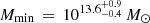 and suggesting that the lensing effect is produced by a cluster-size halo near the QSOs positions. Furthermore, Cueli et al. (2021) assessed the potential of magnification bias CCF measurements as a way of constraining the halo mass function according to two common parametrisations (the Sheth & Tormen and the Tinker fits), finding general agreement with traditional values along with a hint at a slightly higher number of halos at intermediate and high masses for the Sheth & Tormen fit.
Since the gravitational deflection of light travelling close to the lenses depends on cosmological distances and galaxy halo properties, magnification bias can be used as an independent cosmological probe to address the estimation of the parameters in the standard cosmological model. In Bonavera et al. (2020), the measurements of this observable are used in a proof of concept with the purpose of constraining some cosmological parameters, finding interesting limits for ΩM ( > 0.24 as a 95% C.I.) and σ8 (< 1.0 as a 95% C.I.). Finally, in González-Nuevo et al. (2021), different biases in the source samples are analysed and corrected in order to obtain the optimal strategy to precisely measure and analyse unbiased CCFs at cosmological scales. Even if measurements based on different observables (CMB anisotropies, Big Bang nucleosynthesis, SNIa observations, BAOs; Hinshaw et al. 2013; Planck Collaboration XIII 2016; Planck Collaboration VI 2020; Fields & Olive 2006; Betoule et al. 2014; Ross et al. 2015) are in general agreement with the current lambda cold dark matter (ΛCDM) model, the need for independent cosmological probes is driven by the fact that recently there have been some hints that suggest a modification of this framework, such as the Hubble constant’s differing measurements (H0 = 74.03 ± 1.42 km s−1 Mpc−1 and 67.4 ± 0.5 km s−1 Mpc−1 by Riess et al. (2019) and Planck Collaboration VI (2020), respectively) and the degenerate ΩM and σ8 relationship (e.g., Heymans et al. 2013; Planck Collaboration XXIV 2016; Hildebrandt et al. 2017; Planck Collaboration VI 2020).
A plethora of works have addressed the issue of probing the distribution of mass in the Universe via measurements of cosmic shear, the gravitational lensing effect causing a coherent distortion of galaxy images. Performed for the first time at the beginning of the millennium (Bacon et al. 2000; Van Waerbeke et al. 2000; Wittman et al. 2000; Rhodes et al. 2001), cosmic shear measurements have benefited from a rapid and considerable refinement of its methodology in order to analyse the results from recent weak lensing surveys such as the Dark Energy Survey (DES; Dark Energy Survey Collaboration 2016), the Kilo-Degree Survey (KiDS; de Jong et al. 2013), and the Hyper Suprime-Cam survey (HSC; Aihara et al. 2018). Constraints on ΩM, σ8, and the dark energy equation-of-state parameter (ω) have thus been obtained in recent works (e.g., Hildebrandt et al. 2017; Troxel et al. 2018; Hikage et al. 2019) by means of a tomographic analysis, that is, by splitting the redshift distribution of galaxies in several bins and measuring the shear CCF between galaxies in different bins (Hu 1999).
Analogously to what is done in shear studies, a tomographic analysis might improve the results on the cosmological parameters, particularly by allowing a better estimation of the halo occupation distribution (HOD) parameters. Slightly different values for these parameters are expected when probed in separate redshift bins. This is demonstrated in González-Nuevo et al. (2017), where tomographic studies on the HOD parameters are also performed by splitting the foreground sample in four bins of redshift, namely 0.1 < z < 0.2, 0.2 < z < 0.3, 0.3 < z < 0.5 and 0.5 < z < 0.8. It has been found that while  is almost redshift independent, there is a clear evolution in
  , which increases with redshift in agreement with theoretical estimations. Moreover, González-Nuevo et al. (2021) use a background sample of the Herschel Astrophysical Terahertz Large Area Survey (H-ATLAS) galaxies with photometric redshifts z > 1.2 and two independent foreground samples, Galaxy And Mass Assembly (GAMA) galaxies with spectroscopic redshifts and Sloan Digital Sky Survey (SDSS) galaxies with photometric redshifts, with 0.2 < z < 0.8 in order to perform a simplified tomographic analysis, obtaining constraints on the cosmological parameters ΩM (
 ) and σ8 (
 ) as a 68% C.I.
This work constitutes a step forward from Bonavera et al. (2020). We explore the possibility of improving the constraints on ΩM, σ8, and H0 by adopting the unbiased samples of González-Nuevo et al. (2021) and introducing a tomographic analysis by jointly estimating the HOD parameters in four different bins of redshift along with the aforementioned cosmological parameters. We also add the possibility of allowing different values for the dark energy equation of state parameter, ω, to study the possible redshift evolution of the predominant energy contribution of the Universe.
For a flat cosmology with a constant dark energy equation of state, Allen et al. (2008) found ω = −1.14 ± 0.31, using Chandra measurements of the X-ray gas mass fraction in 42 galaxy clusters. When combining their data with independent constraints from cosmic microwave background and SNIa studies, they obtain improved value of ω = − 0.98 ± 0.07. In Suzuki et al. (2012), for the same constant-ω model, SNe Ia alone give 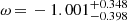 and SNe combined with the constraints from BAO, CMB, and H0 measure
 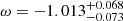 (68% C.I.). Planck Collaboration VI (2020) set the tightest constraints from the combination of Planck TT,TE,EE+lowE+lensing+SNe+BAO to ω0 = −1.03 ± 0.03, but when using Planck TT,TE,EE+lowE+lensing alone is considerably less constraining (see Fig. 30 in Planck Collaboration VI 2020); for example, they obtain
 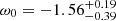 (68% C.I.) with the baseline model base_w_plikHM_TT_lowl_lowE. When the ωa parameter is not fixed to ωa = 0, they find the tightest constraints for the data combination Planck TT,TE,EE+lowE+lensing+BAO+SNe to ω0 = − 0.957 ± 0.080 and
 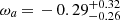 (68% C.I.), but ω0 = −0.76 ± 0.20 and
 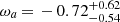 (68% C.I.) Planck+BAO/RSD+WL (see Table 6 in Planck Collaboration VI 2020) and
 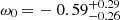 and ωa = − 1.33 ± 0.79 (68% C.I.) for the baseline base_w_wa_plikHM_TT_lowl_lowE_BAO (parameter grid table in the PLA).
For ωaAlam et al. (2017) find a value of −0.39 ± 0.34 with a cosmological analysis of BOSS Galaxies combining Planck+BAO+FS+SN and a value of −1.16 ± 0.55 with Planck+BAO. They also find a strong ω0 − ωa correlation.
Results on the ω parameter have also been provided by the Dark Energy Survey (DES Abbott et al. 2018) Year1. From a starting point using only the Y1 ξ±(θ) information, a value was found of 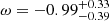 at 68% C.I. By combining different observations, the best finding is
  for the DES Y1+Planck+JLA+BAO combination at 68% C.I. An improvement of 12% is reported by Porredon et al. (2021) from the combination of galaxy clustering and galaxy-galaxy lensing by optimising the lens galaxy sample selection using information from DES Year3 data and assuming the DES Year1 METACALIBRATION sample for the sources. Recently, DES Collaboration (2021) have found a value of
  with the DES Y3 3×2pt analysis.
This paper is organised as follows. Section 2 provides a description of the data used in this work. Section 3 presents the methodology we followed in the measurement, modelling, and study of our observable. The results we obtained on the astrophysical constraints with a fixed ΛCDM cosmology are described in Sect. 4, and those on the cosmological constraints in Sect. 5. Finally, Sect. 6 summarises the conclusions that can be drawn from our findings.
2. Data
In this work we use the same background and foreground samples as in Bonavera et al. (2020), and the CCF data are computed according to the mini-Tiles scheme detailed in González-Nuevo et al. (2021). We prefer the mini-Tiles to the Tiles scheme because of the minimum surface area corrections required and the better statistics (about 96 mini tiles of ≈2 × 2 deg2, to be compared with about 24 different tiles of ≈4 × 4 deg2 each).
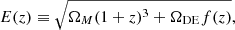
The foreground sources are selected in the GAMA II spectroscopic survey (Driver et al. 2011; Baldry et al. 2010, 2014; Liske et al. 2015). They consist of ∼225 000 galaxies with spectroscopic redshifts of 0.1 < z < 0.8 and a median value of zmed = 0.28. The same sample was used in González-Nuevo et al. (2017, 2021), and Bonavera et al. (2020), and is referred to as the zspec sample in the last of the three. In this work we divided the foreground sample into four redshift bins: 0.1 − 0.2, 0.2 − 0.3, 0.3 − 0.5, and 0.5 − 0.8. These redshift ranges were chosen in order to obtain a similar number of sources in each bin. Moreover, with respect to our previous works, we included sources at lower redshifts (0.1–0.2) in order to add some potentially useful information for the tomographic analysis. Figure 1 shows the redshift distribution of the background sources and the regions that represent the four selected bins of redshift. Since the spectroscopic redshifts for the foreground sources have negligible errors, there is no overlap in the redshift distribution among bins and no source is misplaced in the wrong bin.
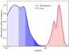 |
Fig. 1. Normalised redshift distribution of the background (red line) and foreground (blue line) samples. The coloured areas represents the selected ranges of redshift: in red the 1.2 < z < 4.0 interval for the background SMGs sample and in different shades of blue the 0.1 < z < 0.2, 0.2 < z < 0.3, 0.3 < z < 0.5, and 0.5 < z < 0.8 bins for the foreground GAMA galaxies. |
The background sample consists of Herschel (Pilbratt et al. 2010; Eales et al. 2010) sources detected in the three GAMA fields (total area of ∼147 deg2) and the part of the south galactic region (SGP) that overlaps with the foreground sample (∼60 deg2). Details concerning the generation of the H-ATLAS catalogue can be found in Ibar et al. (2010), Pascale et al. (2011), Rigby et al. (2011), Valiante et al. (2016), Bourne et al. (2016), and Maddox & Dunne (2020). A photometric redshift selection of 1.2 < z < 4.0 has been applied to ensure no overlap in the redshift distributions of lenses and background sources (red area in Fig. 1), thus being left with 57930 galaxies (∼24% of the initial sample). The process of redshift estimation is described in detail in González-Nuevo et al. (2017) and Bonavera et al. (2019). It consists in a minimum χ2 fit to the SPIRE data, and to PACS data when available, of the SMM J2135-0102 template SED (the Cosmic Eyelash at z = 2.3; Ivison et al. 2010; Swinbank et al. 2010). It has been found to be the best overall template having Δz/(1 + z) = − 0.07 with a 0.153 dispersion (Ivison et al. 2016; Lapi et al. 2011; González-Nuevo et al. 2012).
The background redshift distribution used during the analysis (red line) is the estimated p(z|W) of the galaxies selected by our window function (i.e. a top hat for 1.2 < z < 4.0), taking into account the effect of random errors in photometric redshifts on the redshift distribution, as done in González-Nuevo et al. (2017). In the same work it is concluded that the possible cross-contamination (sources at lower redshift, z < 0.8, with photometric redshifts > 1.2) can be considered statistically negligible even when considering the photometric redshift uncertainties (see González-Nuevo et al. 2017, and references therein).
3. Methodology
3.1. Foreground angular auto-correlation function
First of all, we performed an auto-correlation analysis on the GAMA sample to obtain a first estimate of the HOD parameters for the foreground sample. As in Bonavera et al. (2020), we relied just on the H-ATLAS fields G09, G12, and G15 and selected the normalising redshift quality (column NQ) greater than 2 and the spectroscopic redshift (column Z) in the range 0.05 < zspec < 0.6, resulting in a sample with zmed = 0.23.
In each field the number density of galaxies is estimated as Vfield = Afield ⋅ ΔdC, where ΔdC is the comoving distance difference between the chosen maximum and minimum redshifts and Afield is the area of the field, computed as in Bonavera et al. (2020). The angular auto-correlation function w(θ) is estimated with the Landy-Szalay estimator (Eq. (1), Landy & Szalay 1993),
 (1)
(1)
where DD, DR, and RR are the normalised data-data, data-random, and random-random pair counts for a given angular separation θ. Its errors are obtained by extracting 128 bootstrap samples from each field.
According to the halo model formalism (see e.g., Cooray & Sheth 2002), the average number density of galaxies at a given redshift can be expressed as
 (2)
(2)
where n(M, z) is the halo mass function, which we assume to match the Sheth & Tormen fit in this work (Sheth & Tormen 1999), and Ng(M) = Ncen(M)+Nsat(M) is the mean number of galaxies in a halo of mass M, which we split into contributions from central and satellite galaxies, respectively. As in Bonavera et al. (2020), we adopt the three-parameter (α, Mmin, M1) HOD model by Zheng et al. (2005), where Mmin is the minimum halo mass required to host a (central) galaxy, and M1 and α describe the power-law behaviour of satellite galaxies: Nsat(M) = (M/M1)α. Moreover, we assume the projected two-point correlation function (obtained using the standard Limber approximation), w(rp, z), approximately constant in the given redshift bins [z1, z2]. This is a good approximation considering that the auto-correlation varies less than 10% between different bins, and thus even less inside a single bin (see Fig. A.1). In any case, the variation is smaller than the error bars. Therefore, the angular auto-correlation function can be approximated as
![Mathematical equation: $$ \begin{aligned} { w} ( \theta , z ) \approx \biggl [ \int _{z_1}^{z_2} \,\text{ d}z \dfrac{\,\text{ d}V(z)}{\,\text{ d}z} n_f^2(z) \biggr ] \cdot { w}[ r_p( \theta ), \overline{z} ) ] = A \cdot { w}[ r_p( \theta ), \overline{z} ) ] ,\end{aligned} $$](/articles/aa/full_html/2021/12/aa41521-21/aa41521-21-eq17.gif) (3)
(3)
where dV/dz is the comoving volume unit, nf(z) is the normalised redshift distribution of the foreground population, and  denotes the mean redshift of the interval. In this way the normalisation factor, A, can be taken into account as a free parameter along with Mmin, M1, and α, which simplifies and speeds up the calculations.
3.2. Foreground-background angular CCF
Having performed a preliminary analysis of the auto-correlation within the foreground sample, we now turn to the corresponding analysis with the CCF, the actual main observable we mean to probe. As described in detail in González-Nuevo et al. (2017) and Bonavera et al. (2020), its measurement is performed via a modified version of the Landy & Szalay (1993) estimator (Herranz et al. 2001),
 (4)
(4)
where DfDb, DfRb, DbRf, and RfRb are the normalised foreground-background, foreground-random, background-random, and random-random pair counts for a given angular separation θ.
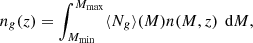
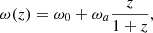
The tiles scheme is the one described in González-Nuevo et al. (2021) and referred to as mini-Tiles therein, shown with red points in Fig. 2. The selected redshift bins are 0.1 − 0.2 (top left), 0.2 − 0.3 (top right), 0.3 − 0.5 (bottom left), and 0.5 − 0.8 (bottom right). The measurement was computed as in Bonavera et al. (2020), the only difference being that median values were preferred because splitting the data into bins of redshifts reduces the statistics. For each redshift bin, we jointly estimate the corresponding HOD parameters together with the cosmological parameters. The only difference with respect to the auto-correlation analysis is that, in the CCF case, the HOD describes only those galaxies and satellites acting as lenses, not the statistical properties of the full sample.
 |
Fig. 2. CCF data computed on Herschel SMGs (as background sample) and GAMA galaxies (as lenses sample) in the mini-Tiles data sets (red points) for the different redshift bins (from left to right, top to bottom): 0.1–0.2 (Bin1), 0.2–0.3 (Bin2), 0.3–0.5 (Bin3), and 0.5–0.8 (Bin4). The empty circles are the data discarded from the MCMC analysis, as explained in the text. The best fits performed in this work are also shown: the runs allowing for astrophysical parameters only (solid line) and for astrophysical and cosmological parameters: σ8, ΩM, and h (dotted line); σ8, ΩM, h, and ω0 (dashed line); and σ8, ΩM, h, ω0, and ωa (dash-dotted line). In the left panel the peaks of the marginalised 1D posterior distributions are used, and in the right panel the mean is used. |
For the theoretical description, we adopt once again the halo model formalism by Cooray & Sheth (2002), as in González-Nuevo et al. (2017) and Bonavera et al. (2019, 2020), and compute the foreground-background source CCF adopting the standard Limber (Limber 1953) and flat-sky approximations (see e.g., Kilbinger et al. 2017, and references therein) as
 (5)
(5)
where
![Mathematical equation: $$ \begin{aligned} W^{\mathrm{lens}}(z)=\frac{3}{2}\frac{H_0^2}{c^2}\bigg [\frac{E(z)}{1+z}\bigg ]^2\int _z^{\infty } \mathrm{d}z^{\prime } \frac{\chi (z)\chi (z^{\prime }-z)}{\chi (z^{\prime })}n_b(z^{\prime }), \end{aligned} $$](/articles/aa/full_html/2021/12/aa41521-21/aa41521-21-eq21.gif) (6)
(6)
nb(z) (nf(z)) is the unit-normalised background (foreground) redshift distribution, χ(z) is the comoving distance to redshift z, J0 is the zeroth-order Bessel function of the first kind, and β is the logarithmic slope of the background sources number counts N(S) = N0S−β, which is assumed to be β = 3 (as in Lapi et al. 2011, 2012; Cai et al. 2013; Bianchini et al. 2015, 2016; González-Nuevo et al. 2017; Bonavera et al. 2019). The quantity
which neglects all contributions to the energy density from curvature or radiation, includes a redshift-dependent function f(z) that considers the potential time evolution of the dark energy density. By assuming that the barotropic index of dark energy is given by
 (7)
(7)
one easily obtains that the dark energy density evolves with redshift as ρ(z) = ρ0f(z), where
 (8)
(8)
and ρ0 is the dark energy density at z = 0. Equivalently, the redshift evolution of the dark energy density parameter is given by
 (9)
(9)
It should be noted that the cosmological constant is recovered by setting ω0 = −1 and ωa = 0.
Some comments should be made regarding the halo modelling of the galaxy-dark matter power spectrum in Eq. (5), Pgal − dm(k, z). As in the auto-correlation analysis, we use the HOD model of Zheng et al. (2005) to describe how galaxies populate dark matter halos. Additionally, halos are identified as spherical regions with an overdensity equal to its virial value, which is estimated at every redshift using the approximation of Weinberg & Kamionkowski (2003). We adopt the usual NFW halo density profile (Navarro et al. 1996) and concentration parameter given in Bullock et al. (2001).
Lastly, the cross-correlation is computed between each individual bin and the background sample, and not among the different bins. Thus, there are only two possible ways to introduce a cross-contamination between different foreground bins. The first, only important at small angular scales, would be the unlikely double lensing event or the alignment along the line of sight of at least three galaxies: two lenses in two different bins of the foreground sample and a source from the background sample. Considering the typical lensing probability, 𝒪(10−3), the double-lensing probability would be of 𝒪(10−6), thus completely negligible from the statistical point of view.
The second possibility is related to a background source amplified by a lens belonging to a higher redshift bin that appears by chance at intermediate angular separation from a foreground galaxy belonging to a lower redshift bin. From the point of view of the lower redshift bin sample, as the lens and the foreground galaxy are not physically related, this magnified background source is indistinguishable from the other background field galaxies. In other words, this background source is taken into account both from the data and the random pairs counting, cancelling out any potential contribution to the final measured CCF for the lower redshift bin sample. For this reason, this second potential cross-contamination is also negligible. Therefore, the CCFs estimated for the different foreground redshift bins can be considered statistically independent.
3.3. Parameter estimation
The estimation of parameters is carried out via a Markov chain Monte Carlo (MCMC) algorithm, performed using the open source emcee software package (Foreman-Mackey et al. 2013), which is an MIT licensed pure-Python implementation of the Affine Invariant MCMC Ensemble sampler by Goodman & Weare (2010). In each MCMC run the number of walkers is set to four times the number of parameters to be estimated, N, and the number of iterations is chosen between 3000 and 5000. Therefore, up to 20000N posterior samples are generated per run. With these posteriors, we then compute an average autocorrelation time, τ, of the estimated autocorrelation times for each parameter (with the get_autocorr_time() function). Next we process the MCMC output by introducing a burn-in of 2τ and a thinning of τ/2 when flattening the chain1. The resulting chains differ in length for each case, which depends not only on the different number of walkers used in the MCMC run, but also on the τ value on each case. We lastly test the convergence of the chains using GETDIST (Lewis 2019).
As already discussed, in the most basic run the astrophysical parameters to be estimated in our analysis are Mmin, M1, and α (different for each redshift bin), while the cosmological parameters are ΩM, σ8, and h (defined via H0 = 100 h km s−1Mpc−1) since with the current samples we cannot constrain Ωb, ΩDE, and ns yet. Consequently, we assume a flat universe with ΩDE = 1 − ΩM and keep the rest fixed to the best-fit Planck Collaboration VI (2020) values of Ωb = 0.0486 and ns = 0.9667. As already explained, this tomographic analysis also introduces the possibility of a redshift variation of the dark energy density and allows us to explore beyond ΛCDM by estimating the ω0 and ωa parameters, according to Eq. (7). Moreover, given that we are in the weak lensing approximation (see Bonavera et al. 2019, for a detailed discussion), only the CCF data in this regime (θ ≥ 0.2 arcmin) are being taken into account (red filled circles in Fig. 2).
Within the Bayesian approach to parameter estimation, both a prior and a likelihood distribution need to be specified. For the latter a traditional Gaussian likelihood function is used. Taking into account the spectroscopic redshifts of the foreground sample (i.e. no overlap between bins) and that the different CCFs can be considered statistically independent (i.e. negligible cross-contamination), there is no need to take into account the covariance inside the likelihood function.
With regard to the selection of the astrophysical parameter priors, we perform a preliminary MCMC run on astrophysical parameters only (setting all cosmological parameters to Planck values) with flat (uniform) priors on each redshift bin corresponding to those of Bonavera et al. (2020). With this test we conclude that Bin 1 results indicate lower masses for the lenses: the galaxies in this redshift bin are very local, so their mass is smaller than that estimated in Bonavera et al. (2020) and we need a smaller value for Mmin. On the other hand, Bin 4 needs higher priors for Mmin: either the mass of the lenses is bigger at higher redshifts or we need higher mass to measure the lensing effect. As a consequence, considering that masses are likely to increase with redshift, we decide to set the following uniform priors for the astrophysical parameters in redshift bin i:
log Mmin ∼ 𝒰[ai, bi], where
![Mathematical equation: $$ \begin{aligned}&[a_1,b_1]=[10.0,13.0]\quad [a_2,b_2]=[11.0,13.0],\\&[a_3,b_3]=[11.5,13.5]\quad [a_4,b_4]=[13.0,15.5]; \end{aligned} $$](/articles/aa/full_html/2021/12/aa41521-21/aa41521-21-eq26.gif)
log M1 ∼ 𝒰[ci, di], where
![Mathematical equation: $$ \begin{aligned}&[c_1,d_1]=[12.0,15.5]\quad [c_2,d_2]=[12.0,15.5],\\&[c_3,d_3]=[12.5,15.5]\quad [c_4,d_4]=[13.0,15.5]; \end{aligned} $$](/articles/aa/full_html/2021/12/aa41521-21/aa41521-21-eq27.gif)
and α ∼ 𝒰[0.5, 1.5] for all bins. Such values are different from the flat priors ranges set for the auto-correlation case (log Mmin ∼ 𝒰[9, 16], log M1 ∼ 𝒰[9, 16] and α ∼ 𝒰[0.1, 2.5]): they are still included in the wider auto-correlation priors, but knowing already the outcome of the preliminary run, they have been chosen to be smaller in order to avoid possible waste of iteration in the runs. As regards the prior distributions of the cosmological parameters to be estimated, they are set to the same ones used in Bonavera et al. (2020): ΩM ∼ 𝒰[0.1 − 0.8], σ8 ∼ 𝒰[0.6 − 1.2], and h ∼ 𝒰[0.5 − 1.0]. The ω0 and ωa uniform priors were chosen to follow the 𝒰[−2.0, 0.0] and 𝒰[−3.0, 3.0], respectively.
4. Astrophysical constraints with fixed ΛCDM cosmology
This section is dedicated to discussing the results from runs where the astrophysical parameters were the only free parameters within a PlanckΛCDM cosmology using the auto- and cross-correlation function measurements. The corner plots and more detailed results of all the cases described here are provided in Appendices A and B.
4.1. Auto-correlation analysis
The priors and results for the auto-correlation run are listed in Table A.1: from left to right, the columns denote the redshift bin, the parameter in question, its prior distribution and the mean (μ), median, 68% credible interval and peak of its marginalised 1D posterior distribution. Figure 3 depicts the one-dimensional posterior distributions of the astrophysical parameters for this run: from left to right, log Mmin, log M1, and α for Bin 1 (black solid line), Bin 2 (red dashed line), Bin 3 (blue dotted line), and Bin 4 (green dash-dotted line).
 |
Fig. 3. One-dimensional posterior distributions of the HOD parameters log(Mmin/M⊙), log(M1/M⊙), and α (from left to right) in each redshift bin for the auto-correlation run. Results for Bins 1–4 are depicted as black solid, red dashed, blue dotted, and green dash-dotted lines, respectively. |
An increase with redshift in log Mmin is observed, the peak in the posterior distributions being at values of 11.55, 11.95, 12.60, and 13.38, from Bin 1 to Bin 4. This is due to a typical selection effect: at a higher redshift, objects with a higher luminosity are more likely to be observed (see Fig. 23 in Driver et al. 2011). The same increase is present in the plot for log M1, peaking at 12.74, 13.06, and 13.76 in Bin 1, Bin 2, and Bin 3, respectively. This parameter does not display a peak for Bin 4, as happens for α, which cannot be constrained in this redshift interval. As regards the rest of the bins, α peaks at almost the same value in Bin 1 and Bin 2 (1.07 and 1.08, respectively) and at a slightly higher value (1.28) in Bin 3.
4.2. CCF analysis
As already discussed, we first performed a MCMC run on only the astrophysical parameters in all four redshift bins, the cosmology being fixed to Planck values. The resulting corner plots for each bin are depicted in Fig. B.1, and the corresponding marginalised posterior distributions are summarised in Table B.1. The one-dimensional posterior distributions for the log Mmin, log M1, and α parameters are shown in Fig. 4 (from left to right) for the four different bins (black solid, red dashed, blue dotted, and green dash-dotted lines for Bin 1, 2, 3, and 4, respectively).
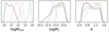 |
Fig. 4. One-dimensional posterior distributions of the HOD parameters log(Mmin/M⊙), log(M1/M⊙) and α (from left to right) in each redshift bin for the CCF run with a fixed cosmology. Results for Bins 1–4 are depicted as black solid, red dashed, blue dotted and green dash-dotted lines, respectively. |
The results regarding Mmin show a general agreement with what is found in the auto-correlation run. The wider distributions still indicates an increase with redshift, and although Bin 1 results are not informative (only providing a 68% upper limit of 11.09), Bin 2 and Bin 3 peak at 11.80 and 12.54, respectively, and a slight disagreement can be observed for Bin 4, which peaks at 13.69.
The results for M1 are generally different with respect to the auto-correlation case, where the increase with redshift is highlighted in Fig. 3. In particular, in Bin 1 and Bin 2 not much can be said about the posterior distributions (lower limits at 13.28 and 13.56, respectively). Moreover, Bin 3 peaks at 12.95 and Bin 4 at 14.09, contrary to the auto-correlation results, which provide just a lower limit. Concerning the α parameter, Bin 3 is the only one showing a peak at 1.16 in the marginalised posterior distribution, being the results on the rest of the bins inconclusive. A similar trend is found by González-Nuevo et al. (2017): they obtain  and
and  for Bin 1,
  and
and  for Bin 2,
  and
and  for Bin 3, and
  and
and  for Bin 4. The results are also in agreement with those from the corresponding non-tomographic run by Bonavera et al. (2020): they give
  and
and  at 68% C.I.
Therefore, there is a clear disagreement between the CCF and the auto-correlation results. This is not unexpected since the CCF is related only to the characteristics of the lenses and not to those of the global sample. From the point of view of the CCF, those foreground galaxies not acting as lenses are invisible or non-existent, and they only contribute to the random part. For example, the higher Mmin value in the last bin with respect to the auto-correlation case suggests that, at a higher redshift (with respect to the other three bins), the mass of the object acting as a lens is higher than the average mass of the whole Bin 4 sample. This is due to the fact that, at a greater distance, only the most massive objects can actually act as lenses in order to compensate the lower lensing probability (Lapi et al. 2012; González-Nuevo et al. 2017). We therefore think that it is not safe to use the auto-correlation results as Gaussian priors on the astrophysical parameters for the cosmological runs, or even to perform a joint analysis, since they might be non-representative of the lens sample in the CCF data. Any use of information from the auto-correlation analysis would introduce an uncontrollable bias in the cosmological results. Moreover, given the tight auto-correlation HOD constraints, they will completely overrun the cosmological analysis if used as Gaussian priors or in a joint analysis. For these reasons we decide to focus on the CCF measurements and to only perform runs with uniform HOD priors in this work.
5. Cosmological constraints
This section constitutes the core of this work. We study the cosmological constraints that can be derived from the measured CCFs. We performed a series of MCMC runs on the HOD and cosmological parameters jointly under the assumptions of different cosmological models (ΛCDM, ω0CDM, and ω0ωaCDM). In particular, we focus on the cosmological parameters ΩM, σ8, h, ω0, and ωa, to whose effect the CCF is more sensitive, while keeping the rest fixed to Planck values. The corner plots and more detailed results of all the cases described here are provided in Appendix B.
5.1. ΛCDM model vs ω0CDM and ω0ωaCDM models
We performed three different MCMC runs: the first within the ΛCDM cosmology (i.e. setting ω0 and ωa to −1 and 0, respectively); the second within the so-called flat ω0CDM model (where ω0 is a free parameter, but ωa is set to 0); and the third and most general model, a flat ω0ωaCDM model (where both parameters are left free). In all three runs the astrophysical HOD parameters are also allowed to vary in the different ranges we discussed in Sect. 3.3.
The derived marginalised posterior distributions of the astrophysical log Mmin (first column) and log M1 (second column) parameters in each redshift bin (1–4, from top to bottom) are compared in Fig. 5 (α is not shown because it is unconstrained in most of the cases). We also add the results from the fixed cosmology case (see Sect. 4). There is overall agreement among all cases.
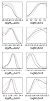 |
Fig. 5. One-dimensional posterior distributions for log(Mmin/M⊙) (first column) and log(M1/M⊙) (second column) in Bins 1, 2, 3, and 4 (from top to bottom, respectively) for the run on just the HOD parameters (black solid lines) and for the three runs on the astrophysical and cosmological parameters jointly, namely within ΛCDM (red dashed lines), within ω0CDM (blue dotted lines), and within ω0ωaCDM (green dash-dotted lines). |
On the other hand, Fig. 6 compares the corresponding results for the cosmological ΩM, σ8 and h parameters (from left to right, respectively) of the three cosmological models assumed in this subsection (depicted as before with red dashed, blue dotted, and green dash-dotted lines) with the previous results by Bonavera et al. (2020) (shown in solid black).
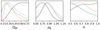 |
Fig. 6. One-dimensional posterior distributions of ΩM, σ8, and h (from left to right) for the results in Bonavera et al. (2020) (black solid lines), and for the three MCMC runs performed jointly on the astrophysical and cosmological parameter in this work, namely within ΛCDM (red dashed lines), within ω0CDM (blue dotted lines), and within ω0ωaCDM (green dash-dotted lines). |
The results for the ΛCMD model, which includes only ΩM, σ8, and h in the cosmological analysis, are shown in Fig. B.2 and Table B.2. The trend for the astrophysical parameters (see red dashed line in Fig. 5) is similar to the fixed cosmology run in Sect. 4. For the cosmological parameters, there is a substantial improvement with respect to the non-tomographic analysis carried out in Bonavera et al. (2020) (black solid line in Fig. 6). They obtain a lower limit of 0.24 at 95% C.I. on ΩM, only a tentative peak around 0.75 for σ8 with an upper limit of 1 at 95% C.I., while we have a detection of ΩM = 0.33 [0.17, 0.41] (mean value and 68% C.I.) and a maximum in the posterior distribution at 0.26. We note that the preference for lower values of ΩM in the present analysis with respect to Bonavera et al. (2020) is a consequence of a better treatment of the estimator biases (González-Nuevo et al. 2021). We also report a constraint on σ8 of 0.87 [0.75, 1.0] at 68% C.I. The ΩM and σ8 values are respectively slightly lower and higher than those found in González-Nuevo et al. (2021) (0.50 and 0.75, respectively). However, when opening the dark energy related parameters, the constraints on σ8 and ΩM loosen, especially that on ΩM. In the ΛCDM case the one-dimensional plots in Fig. 6 (red dashed lines) display clear peaks except in the case of the h parameter, where we just obtain a low significant peak at 0.67 for h.
The corresponding corner plots and summarised results from the ω0CMD model, which allows the ω0 parameter to be free while keeping ωa fixed to 0, are shown in Fig. B.3 and Table B.3. The trend for the parameter distributions in this second case (blue dotted lines in Figs. 5 and 6) is similar to the ΛCDM case. The only exceptions are a broader posterior distribution for Mmin in Bin2 and Bin4, a clear peak for M1 in Bin 2 (there is no peak in the ΛCDM case), and h, which is not constrained, showing a preference towards lower values. In particular, the ΩM and σ8 parameters peak at 0.26 and 0.85, respectively (being compatible with the findings of the ΛCDM case).
The results from the third and most general model ω0ωaCDM, which gives freedom to both ω0 and ωa are shown in Fig. B.4 and Table B.4. As shown in Figs. 5 and 6 (green dash-dotted lines), there is overall agreement with the other cases: we obtain peaks for ΩM and σ8 at 0.21 and 0.84, respectively, which are slightly lower than the other cases. Instead, h is unconstrained, favouring lower values as in the other cases.
The contour plots of the two-dimensional posterior distribution for ΩM and σ8 in all three cases are shown in Fig. 7 (in green, red, and blue, respectively)2. For comparison purposes, the results by Bonavera et al. (2020) are also shown (in black). As in Fig. 6, the improvement with respect to previous results with magnification bias can be appreciated: the lower limit on ΩM is still present, especially in the ΛCDM case and even if it lowers and worsens in the ω0CDM and ω0ωaCDM cases (see Tables B.3 and B.4, respectively), they are in general more constraining in the ΩM-σ8 plane with respect to the non-tomographic case. On the other hand, upper constraints to the distributions are achieved in the tomographic case with the three runs.
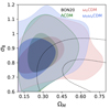 |
Fig. 7. Contour plot of the two-dimensional posterior distribution of ΩM and σ8 for the three MCMC runs where the astrophysical and cosmological parameters are jointly analysed, namely within ΛCDM (in green), within ω0CDM (in red), and within ω0ωaCDM (in blue). Moreover, in order to compare with previous results, those by Bonavera et al. (2020) are shown in black. The contours are set to 0.393 and 0.865. |
The best-fit models for the CCFs obtained in all these cases are shown in Fig. 2. In the left panel we use the peak of each one of the marginalised 1D posterior distributions (although it is not the same as the maximum of the n-dimensional posterior distribution), while we use the associated mean values for the right panel. In particular, the solid line represents the results from the fixed cosmology case whereas the dotted, dashed, and dash-dotted lines are used for the three runs where cosmology was taken into account (ΛCDM, ω0CDM, and ω0ωaCDM, respectively). When using the maxima of the posterior distributions, the fixed cosmology results provides the lowest curves while the ω0ωaCDM one the highest. On the other hand, when using the mean values major differences among the different runs are not found.
The reduced χ2 values for the best fits with the mean (peaks values of the 1D posterior distributions) are 0.36 (0.54), 0.44 (1.42), 0.44 (1.14), and 0.56 (2.86) for the cases of fixed cosmology (36 d.o.f.), ΛCDM (33 d.o.f.), ω0CDM (32 d.o.f.), and ω0ωaCDM (31 d.o.f.), respectively. It should be noted that when using the n-dimensional best fit, the reduced χ2 obviously improves (1.05 for the ω0ωaCDM case). The bigger values for the peaks case are mostly due to the worst best fit in Bin 3. It is interesting that the ω0CDM case has a comparable or better χ2 with respect to the ΛCDM case. It should be noted that emcee is not an optimiser, but a sampler. As such, and in the context of Bayesian statistics, the single tuple of parameters that best fits the data (that is, the maximum of the n-dimensional posterior distribution) cannot be associated with credible intervals for each individual parameter. What can be done is to marginalise over the rest of the parameters in order to obtain one-dimensional distributions, the maximum of which will not, in general, coincide with the individual value of the aforementioned tuple. This explains why χ2 values for individual fits have to be interpreted with care, since the most meaningful information comes from the overall distributions, not from point estimates. In conclusion, the different cases considered in this work show a general agreement regarding the posterior distributions, although there are slight changes in the peak positions, well within 1σ limits in most cases.
5.2. The Dark Energy equation of state
In this subsection we focus on the dark energy equation of state and what we can learn about it from our results. Figure 8 shows the contour plot of the two-dimensional posterior distribution for h and ω0. The results from the run within ω0CDM is shown in red, while those corresponding to ω0ωaCDM are depicted in blue. The green bar represents the run within ΛCDM. We find a mean value of −1.00 and a maximum of the posterior distribution of −0.97 for ω0 ([ − 1.56, −0.47] 68% C.I.) for the ω0CDM model. Under the ω0ωaCDM model we derive −1.09 and −0.92 for ω0 [ − 1.72, −0.66] C.I. and −0.19 and −0.20 for ωa [ − 1.88, 1.48] 68% C.I. for the ω0ωaCDM model.
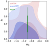 |
Fig. 8. Contour plot of the two-dimensional posterior distribution of h and ω0 for the three MCMC runs where the astrophysical and cosmological parameters are jointly analysed, namely within ΛCDM (in green), the within ω0CDM (in red), and within ω0ωaCDM (in blue). The contours are set to 0.393 and 0.865. |
Moreover, Fig. 9 displays the contour plot of the two-dimensional posterior distribution of ω0 and ωa. There seems to be a degeneracy direction, with ωa having higher values for lower values of ω0. This anti-correlation is at 30%. Taking into account the results from these alternative models (ω0CDM and ω0ωaCDM), our measurements are in agreement with ΛCDM (ω0 = −1 and ωa = 0) at 68% C.I.
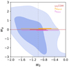 |
Fig. 9. Contour plot of the two-dimensional posterior distribution of ω0 and ωa for the MCMC run within ω0ωaCDM. The contours are set to 0.393 and 0.865. |
However, since the previous cases were not able to constrain the h parameter, we now investigate if ω0 is somehow affected by changes in H0. In order to do so, we performed a MCMC run on the astrophysical parameters and ω0 by fixing the rest of the cosmology to Planck values, and then comparing the results with a similar MCMC run with the exception of H0 being fixed to the value from Riess et al. (2019, H0 = 74.03 ± 1.42 km s−1 Mpc−1).
The results are shown in Figs. B.5 and B.6 and summarised in Tables B.5 and B.6 (for the cases fixing H0 to the Planck and Riess et al. (2019) values, respectively). The marginalised posterior distribution for ω0 peaks at −0.69 ([−1.31, −0.38] at 68% C.I.) and −0.86 ([−1.29, −0.45] at 68% C.I.) for the Planck and Riess value of H0, respectively. These results show that ω0 tends to higher values when the Planck H0 value is used.
However, we note a degeneracy in the ω0 − Mmin plane: a higher ω0 tends to prefer a lower Mmin, a phenomenon that is evident in Bin 3, but especially in Bin 4. In both bins the degeneracy is at about 50%. The same results can also be seen in the previous general runs (see Figs. B.3 and B.4), for both redshift bins. In Bin 4 is where we generally have the greatest difference in Mmin when compared with the auto-correlation results. This difference disappear for higher ω0 values, making Mmin in agreement with the auto-correlation findings.
Therefore, we observe that fixing H0 to the hRiess and hPlanck values produces shifts towards ω0 > −1 values in the derived maximum of the 1D marginalised posterior distribution. However, both cases are still compatible with the ΛCDM model at the 68% C.I.
5.3. Comparison with other results
As in Bonavera et al. (2020), we compare our cosmological constraints with those obtained using the shear of the weak gravitational lensing (some of which are known to be in tension). In particular, Fig. 10 shows the contour plots for the posterior distribution of ΩM and σ8 (68% and 95% C.I., for a direct comparison with the literature, which are different from the values of 39.3% and 86.5% used in the corner plots shown in the previous sections) from the publicly released CMB lensing from Planck (Planck Collaboration VIII 2020, in blue), cosmic shear tomography measurements of the Canada-France-Hawaii Telescope Lensing Survey (CFHTLenS, Joudaki et al. 2017, in cyan), first combined cosmological measurements of the Kilo Degree Survey and VIKING based on 450 deg2 data (KV450, Hildebrandt et al. 2020, in grey), first-year lensing data from the Dark Energy Survey (DES Troxel et al. 2018, in magenta) and two-point correlation functions of the Subaru Hyper Suprime-Cam first-year data (HSC, Hamana et al. 2020, in yellow). For completeness, we also show results from Planck CMB temperature and polarisation angular power spectra (in dark blue). The results of this work are shown in green (ΛCDM).
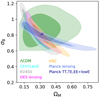 |
Fig. 10. Comparison among the contour plots in the ΩM – σ8 plane from Planck CMB lensing (blue), CFHTLenS (cyan), KV450 (grey), DES (magenta), and HSC (yellow) and the results from this work (green). Differently from the other 2D plots in this work, the contours here are set to 0.68 and 0.95. |
It should be noted that we do not attempt to adjust the different priors to our fiducial set-up as an in-depth comparison is beyond the scope of this paper. Moreover, it should be considered that these results span different redshift ranges and are affected by completely different systematic effects with respect to the magnification bias measurements (which thus represent a complementary probe to weak lensing).
The combination of this external data set identifies degeneracy directions that are clearly visible in Fig. 10. As already anticipated in Bonavera et al. (2020), the tomographic results confirm that the magnification bias does not show the degeneracy found with cosmic shear measurements. In order to further confirm this conclusion, we perform a principal component analysis (PCA) on the ΛCDM results. The first principal component is  , almost orthogonal to the cosmic shear degeneracy. At present this component is constrained at a level of ∼18%, and therefore it cannot be considered a proper degeneracy. Better constraints are needed before deciding if magnification bias results can be further improved by analysing this component, as commonly done with S8 in cosmic shear analyses.
With respect the ω0CDM and ω0ωaCDM models, our results are in agreement with recent findings in literature. They also have a comparable precision when referring to non-combined results from other experiments see Fig. 11 for the ω0 comparison of the 68% C.I. from this work (red bar for the ω0CDM case and yellow one for the ω0ωaCDM case) with findings by other experiments. For example, in the ω0CDM case, Allen et al. (2008) (green bar) obtain ω = −1.14 ± 0.31, Suzuki et al. (2012) (purple bar) 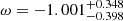 , Planck3
 (baseline base_w_plikHM_TT_lowl_lowE; blue bar), and Abbott et al. (2018) (magenta bar)
  . In the ω0ωaCDM case, Planck3 results obtain
 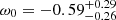 and ωa = −1.33 ± 0.79 (baseline base_w_wa_plikHM_TT_lowl_lowE_BAO; cyan bar). Moreover, the strong degeneracy between ω0 and ωa is also found in Alam et al. (2017) using models that allow the evolving equation of state (see Eq. (7)) in a flat universe, and constraints on ωa are also found to be poor ωa = −0.39 ± 0.34.
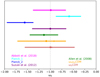 |
Fig. 11. Comparison of ω0 results of this work at 68% C.I. (ω0CDM model in red and ω0ωaCDM model in yellow) with findings from some other experiments: DES (magenta), Planck_1 (baseline base_w_wa_plikHM_TT_lowl_lowE_BAO, cyan), Planck_2 (baseline base_w_plikHM_TT_lowl_lowE, blue), supernovae (purple), x-ray measurements (green). |
Even if our results are not yet very constraining, they put somewhat interesting limits to the other external results and do not present the typical degeneracy that characterises cosmic shear results. It is very likely that in the future, more constraining magnification bias samples can offer a complementary probe able to break the degeneracy and improve the dark energy constraints.
6. Conclusions
In this work we exploited the magnification bias effect, similarly to Bonavera et al. (2020) and following the work by González-Nuevo et al. (2017) and Bonavera et al. (2019) on high-z submillimetre galaxies, to perform a tomographic analysis with a view of searching for constraints on the free parameters of the HOD model (Mmin, M1, and α), but also on the cosmological ΩM, σ8, h, ω0, and ωa parameters in four different cases (fixed cosmology, ΛCDM, ω0CDM, and ω0ωaCDM). To perform this analysis we split the foreground sample into four bins of redshift with approximately the same number of lenses: 0.1–0.2, 0.2–0.3, 0.3–0.5, 0.5–0.8.
For the astrophysical parameters, we could not successfully constrain the α parameters in any of our redshift bins. In some cases the posterior distributions showed a broad peak (e.g., in Bin 3 with a mean value at 1.09 [0.92, 1.43] 68% C.I. for the ω0CDM case). In Mmin we found upper limits in most of the cases for Bin1 (< 10), suggesting that at lower redshifts the average minimum mass needed might be lower than in the other cases and more difficult to constrain, perhaps also due to the larger uncertainties in these data. In Bin2 the situation slightly improved; we obtained broad peaks in all cases at log10(Mmin/M⊙)∼12. In Bin3 and Bin4 the 1D distributions have clear maxima for most of the cases at log10(Mmin/M⊙)∼12.5 and at 13.7, respectively. The results on Mmin confirm the values by González-Nuevo et al. (2017), showing the trend towards higher values at higher redshift. For M1 the situation worsens again, setting lower limits for most of the cases with the exception of Bin3 and Bin4 (peaking at about log10(M1/M⊙)∼13 and 14, respectively).
For the cosmological parameters, for ΩM we obtained somewhat lower values with respect to the González-Nuevo et al. (2021) findings; the highest are the ΛCDM and ω0CDM cases with a maximum at 0.26 and the lowest the ω0ωaCDM case with a maximum at 0.21. On the other hand, we found slightly higher values for σ8, peaking in all cases between 0.84 and 0.87. Unfortunately h is not constrained yet, obtaining just a low significant peak at 0.67 in the ΛCDM case.
The tomographic analysis presented in this work improves the constraints in the σ8 − ΩM plane with respect to Bonavera et al. (2020) and it confirms that magnification bias results do not show the degeneracy found with cosmic shear measurements. Further progress with this approach is subject to the possibility of increasing the statistics in each redshift bin, which is necessary to reduce the uncertainties on the CCF data at large scales.
Moreover, we were able to study the barotropic index of dark energy ω and its possible evolution with redshift, obtaining results in agreement with current findings in literature and with a similar constraining level, finding a peak at −0.97 ([ − 1.56, −0.47] 68% C.I.) and at −0.92 ([ − 1.72, −0.66] 68% C.I.) for ω0 in the ω0CDM and ω0ωaCDM cases, respectively. For ωa we obtain a peak at −0.20 ([ − 1.88, 1.48] 68% C.I.) and a 30% anti-correlation with ω0.
Finally, we explored the impact on ω0 when fixing H0 to either the Planck Collaboration VIII (2020) or the Riess et al. (2019) values. We set the cosmological parameters to the Planck values (Planck Collaboration VIII 2020) and ran only on the HOD parameters and ω0 with H0 first fixed to the value determined by Planck and then to the value by Riess et al. (2019). We found a trend of higher ω0 values for lower H0 values.
As suggested in the tutorials section of the official emcee3.0.2 documentation at https://emcee.readthedocs.io/en/stable/
The 1σ and 2σ levels for the 2D contours are 39.3% and 86.5%, not 68% and 95%. Otherwise, there is no direct comparison with the 1D histograms above the contours.
See the parameter grid tables in the PLA Planck Collaboration. 2018, Planck Legacy Archive, https://pla.esac.esa.int/
Acknowledgments
We deeply thank the anonymous referee for quite useful comments on the original draft. L. B., J. G. N., M. M. C., J. M. C., D. C. acknowledge the PGC 2018 project PGC2018-101948-B-I00 (MICINN/FEDER). M. M. C. acknowledges support from PAPI-20-PF-23 (Universidad de Oviedo). M. M. is supported by the program for young researchers “Rita Levi Montalcini” year 2015 and acknowledges support from INFN through the InDark initiative. A. L. acknowledges partial support from PRIN MIUR 2015 Cosmology and Fundamental Physics: illuminating the Dark Universe with Euclid, by the RADIOFOREGROUNDS grant (COMPET-05-2015, agreement number 687312) of the European Union Horizon 2020 research and innovation program, and the MIUR grant ‘Finanziamento annuale individuale attivita base di ricerca’. We deeply acknowledge the CINECA award under the ISCRA initiative, for the availability of high performance computing resources and support. In particular the projects “SIS19_lapi”, “SIS20_lapi” in the framework “Convenzione triennale SISSA-CINECA”. The Herschel-ATLAS is a project with Herschel, which is an ESA space observatory with science instruments provided by European-led Principal Investigator consortia and with important participation from NASA. The H-ATLAS web-site is http://www.h-atlas.org. GAMA is a joint European-Australasian project based around a spectroscopic campaign using the Anglo-Australian Telescope. The GAMA input catalogue is based on data taken from the Sloan Digital Sky Survey and the UKIRT Infrared Deep Sky Survey. Complementary imaging of the GAMA regions is being obtained by a number of independent survey programs including GALEX MIS, VST KIDS, VISTA VIKING, WISE, Herschel-ATLAS, GMRT and ASKAP providing UV to radio coverage. GAMA is funded by the STFC (UK), the ARC (Australia), the AAO, and the participating institutions. The GAMA website is: http://www.gama-survey.org/. In this work, we made extensive use of GetDist (Lewis 2019), a Python package for analysing and plotting MC samples. In addition, this research has made use of the python packages ipython (Pérez & Granger 2007), matplotlib (Hunter 2007) and Scipy (Jones et al. 2001).
References
- Abbott, T. M. C., Abdalla, F. B., Alarcon, A., et al. 2018, Phys. Rev. D, 98, 043526 [NASA ADS] [CrossRef] [Google Scholar]
- Aihara, H., Arimoto, N., Armstrong, R., et al. 2018, PASJ, 70, S4 [NASA ADS] [Google Scholar]
- Alam, S., Ata, M., Bailey, S., et al. 2017, MNRAS, 470, 2617 [Google Scholar]
- Allen, S. W., Rapetti, D. A., Schmidt, R. W., et al. 2008, MNRAS, 383, 879 [Google Scholar]
- Aretxaga, I., Wilson, G. W., Aguilar, E., et al. 2011, MNRAS, 415, 3831 [Google Scholar]
- Bacon, D. J., Refregier, A. R., & Ellis, R. S. 2000, MNRAS, 318, 625 [NASA ADS] [CrossRef] [Google Scholar]
- Bakx, T. J. L. C., Eales, S., & Amvrosiadis, A. 2020, MNRAS, 493, 4276 [NASA ADS] [CrossRef] [Google Scholar]
- Baldry, I. K., Robotham, A. S. G., Hill, D. T., et al. 2010, MNRAS, 404, 86 [NASA ADS] [Google Scholar]
- Baldry, I. K., Alpaslan, M., Bauer, A. E., et al. 2014, MNRAS, 441, 2440 [Google Scholar]
- Betoule, M., Kessler, R., Guy, J., et al. 2014, A&A, 568, A22 [NASA ADS] [CrossRef] [EDP Sciences] [Google Scholar]
- Bianchini, F., Bielewicz, P., Lapi, A., et al. 2015, ApJ, 802, 64 [NASA ADS] [CrossRef] [Google Scholar]
- Bianchini, F., Lapi, A., Calabrese, M., et al. 2016, ApJ, 825, 24 [NASA ADS] [CrossRef] [Google Scholar]
- Blain, A. W. 1996, MNRAS, 283, 1340 [NASA ADS] [CrossRef] [Google Scholar]
- Bonavera, L., González-Nuevo, J., Suárez Gómez, S. L., et al. 2019, JCAP, 2019, 021 [Google Scholar]
- Bonavera, L., González-Nuevo, J., Cueli, M. M., et al. 2020, A&A, 639, A128 [NASA ADS] [CrossRef] [EDP Sciences] [Google Scholar]
- Bourne, N., Dunne, L., Maddox, S. J., et al. 2016, MNRAS, 462, 1714 [NASA ADS] [CrossRef] [Google Scholar]
- Bullock, J. S., Kolatt, T. S., Sigad, Y., et al. 2001, MNRAS, 321, 559 [Google Scholar]
- Bussmann, R. S., Gurwell, M. A., Fu, H., et al. 2012, ApJ, 756, 134 [CrossRef] [Google Scholar]
- Bussmann, R. S., Pérez-Fournon, I., Amber, S., et al. 2013, ApJ, 779, 25 [NASA ADS] [CrossRef] [Google Scholar]
- Cai, Z.-Y., Lapi, A., Xia, J.-Q., et al. 2013, ApJ, 768, 21 [NASA ADS] [CrossRef] [Google Scholar]
- Calanog, J. A., Fu, H., Cooray, A., et al. 2014, ApJ, 797, 138 [NASA ADS] [CrossRef] [Google Scholar]
- Cooray, A., & Sheth, R. 2002, Phys. Rep., 372, 1 [Google Scholar]
- Cueli, M. M., Bonavera, L., González-Nuevo, J., & Lapi, A. 2021, A&A, 645, A126 [NASA ADS] [CrossRef] [EDP Sciences] [Google Scholar]
- Dark Energy Survey Collaboration (Abbott, T., et al.) 2016, MNRAS, 460, 1270 [Google Scholar]
- de Jong, J. T. A., Kuijken, K., Applegate, D., et al. 2013, Messenger, 154, 44 [Google Scholar]
- DES Collaboration (Abbott, T. M. C., et al.) 2021, ArXiv e-prints [arXiv:2105.13549] [Google Scholar]
- Driver, S. P., Hill, D. T., Kelvin, L. S., et al. 2011, MNRAS, 413, 971 [Google Scholar]
- Dunne, L., Bonavera, L., Gonzalez-Nuevo, J., Maddox, S. J., & Vlahakis, C. 2020, MNRAS, 498, 4635 [NASA ADS] [CrossRef] [Google Scholar]
- Eales, S., Dunne, L., Clements, D., et al. 2010, PASP, 122, 499 [NASA ADS] [CrossRef] [Google Scholar]
- Fields, B. D., & Olive, K. A. 2006, Nucl. Phys. A, 777, 208 [NASA ADS] [CrossRef] [Google Scholar]
- Foreman-Mackey, D., Hogg, D. W., Lang, D., & Goodman, J. 2013, PASP, 125, 306 [Google Scholar]
- Fu, H., Jullo, E., Cooray, A., et al. 2012, ApJ, 753, 134 [NASA ADS] [CrossRef] [Google Scholar]
- González-Nuevo, J., Lapi, A., Fleuren, S., et al. 2012, ApJ, 749, 65 [Google Scholar]
- González-Nuevo, J., Lapi, A., Negrello, M., et al. 2014, MNRAS, 442, 2680 [Google Scholar]
- González-Nuevo, J., Lapi, A., Bonavera, L., et al. 2017, JCAP, 2017, 024 [Google Scholar]
- González-Nuevo, J., Cueli, M. M., Bonavera, L., et al. 2021, A&A, 646, A152 [NASA ADS] [CrossRef] [EDP Sciences] [Google Scholar]
- Goodman, J., & Weare, J. 2010, Commun. Appl. Math. Comput. Sci., 5, 65 [Google Scholar]
- Hamana, T., Shirasaki, M., Miyazaki, S., et al. 2020, PASJ, 72, 16 [Google Scholar]
- Herranz, D. 2001, in Cosmological Physics with Gravitational Lensing, eds. J. Tran Thanh Van, Y. Mellier, & M. Moniez, 197 [Google Scholar]
- Heymans, C., Grocutt, E., Heavens, A., et al. 2013, MNRAS, 432, 2433 [Google Scholar]
- Hikage, C., Oguri, M., Hamana, T., et al. 2019, PASJ, 71, 43 [Google Scholar]
- Hildebrandt, H., van Waerbeke, L., Scott, D., et al. 2013, MNRAS, 429, 3230 [NASA ADS] [CrossRef] [Google Scholar]
- Hildebrandt, H., Viola, M., Heymans, C., et al. 2017, MNRAS, 465, 1454 [Google Scholar]
- Hildebrandt, H., Köhlinger, F., van den Busch, J. L., et al. 2020, A&A, 633, A69 [NASA ADS] [CrossRef] [EDP Sciences] [Google Scholar]
- Hinshaw, G., Larson, D., Komatsu, E., et al. 2013, ApJS, 208, 19 [Google Scholar]
- Hu, W. 1999, ApJ, 522, L21 [Google Scholar]
- Hunter, J. D. 2007, Comput. Sci. Eng., 9, 90 [NASA ADS] [CrossRef] [Google Scholar]
- Ibar, E., Ivison, R. J., Cava, A., et al. 2010, MNRAS, 409, 38 [NASA ADS] [CrossRef] [Google Scholar]
- Ivison, R. J., Swinbank, A. M., Swinyard, B., et al. 2010, A&A, 518, L35 [NASA ADS] [CrossRef] [EDP Sciences] [Google Scholar]
- Ivison, R. J., Lewis, A. J. R., Weiss, A., et al. 2016, ApJ, 832, 78 [Google Scholar]
- Jones, E., Oliphant, T., Peterson, P., et al. 2001, SciPy: Open source scientific tools for Python [Google Scholar]
- Joudaki, S., Blake, C., Heymans, C., et al. 2017, MNRAS, 465, 2033 [Google Scholar]
- Kilbinger, M., Heymans, C., Asgari, M., et al. 2017, MNRAS, 472, 2126 [Google Scholar]
- Landy, S. D., & Szalay, A. S. 1993, ApJ, 412, 64 [Google Scholar]
- Lapi, A., González-Nuevo, J., Fan, L., et al. 2011, ApJ, 742, 24 [NASA ADS] [CrossRef] [Google Scholar]
- Lapi, A., Negrello, M., González-Nuevo, J., et al. 2012, ApJ, 755, 46 [NASA ADS] [CrossRef] [Google Scholar]
- Lewis, A. 2019, ArXiv e-prints [arXiv:1910.13970] [Google Scholar]
- Limber, D. N. 1953, ApJ, 117, 134 [NASA ADS] [CrossRef] [Google Scholar]
- Liske, J., Baldry, I. K., Driver, S. P., et al. 2015, MNRAS, 452, 2087 [Google Scholar]
- Maddox, S. J., & Dunne, L. 2020, MNRAS, 493, 2363 [NASA ADS] [CrossRef] [Google Scholar]
- Ménard, B., Scranton, R., Fukugita, M., & Richards, G. 2010, MNRAS, 405, 1025 [NASA ADS] [Google Scholar]
- Navarro, J. F., Frenk, C. S., & White, S. D. M. 1996, ApJ, 462, 563 [Google Scholar]
- Nayyeri, H., Keele, M., Cooray, A., et al. 2016, ApJ, 823, 17 [NASA ADS] [CrossRef] [Google Scholar]
- Negrello, M., Perrotta, F., González-Nuevo, J., et al. 2007, MNRAS, 377, 1557 [NASA ADS] [CrossRef] [Google Scholar]
- Negrello, M., Hopwood, R., De Zotti, G., et al. 2010, Science, 330, 800 [NASA ADS] [CrossRef] [Google Scholar]
- Negrello, M., Amber, S., Amvrosiadis, A., et al. 2017, MNRAS, 465, 3558 [NASA ADS] [CrossRef] [Google Scholar]
- Pascale, E., Auld, R., Dariush, A., et al. 2011, MNRAS, 415, 911 [NASA ADS] [CrossRef] [Google Scholar]
- Pérez, F., & Granger, B. E. 2007, Comput. Sci. Eng., 9, 21 [Google Scholar]
- Pilbratt, G. L., Riedinger, J. R., Passvogel, T., et al. 2010, A&A, 518, L1 [NASA ADS] [CrossRef] [EDP Sciences] [Google Scholar]
- Planck Collaboration XIII. 2016, A&A, 594, A13 [NASA ADS] [CrossRef] [EDP Sciences] [Google Scholar]
- Planck Collaboration XXIV. 2016, A&A, 594, A24 [NASA ADS] [CrossRef] [EDP Sciences] [Google Scholar]
- Planck Collaboration VI. 2020, A&A, 641, A6 [NASA ADS] [CrossRef] [EDP Sciences] [Google Scholar]
- Planck Collaboration VIII. 2020, A&A, 641, A8 [NASA ADS] [CrossRef] [EDP Sciences] [Google Scholar]
- Porredon, A., Crocce, M., Fosalba, P., et al. 2021, Phys. Rev. D, 103, 043503 [Google Scholar]
- Rhodes, J., Refregier, A., & Groth, E. J. 2001, ApJ, 552, L85 [NASA ADS] [CrossRef] [Google Scholar]
- Riess, A. G., Casertano, S., Yuan, W., Macri, L. M., & Scolnic, D. 2019, ApJ, 876, 85 [Google Scholar]
- Rigby, E. E., Maddox, S. J., Dunne, L., et al. 2011, MNRAS, 415, 2336 [NASA ADS] [CrossRef] [Google Scholar]
- Ross, A. J., Percival, W. J., & Manera, M. 2015, MNRAS, 451, 1331 [NASA ADS] [CrossRef] [Google Scholar]
- Schneider, P., Ehlers, J., & Falco, E. E. 1992, Gravitational Lenses [Google Scholar]
- Scranton, R., Ménard, B., Richards, G. T., et al. 2005, ApJ, 633, 589 [NASA ADS] [CrossRef] [Google Scholar]
- Sheth, R. K., & Tormen, G. 1999, MNRAS, 308, 119 [Google Scholar]
- Suzuki, N., Rubin, D., Lidman, C., et al. 2012, ApJ, 746, 85 [NASA ADS] [CrossRef] [Google Scholar]
- Swinbank, A. M., Smail, I., Longmore, S., et al. 2010, Nature, 464, 733 [Google Scholar]
- Troxel, M. A., MacCrann, N., Zuntz, J., et al. 2018, Phys. Rev. D, 98, 043528 [Google Scholar]
- Valiante, E., Smith, M. W. L., Eales, S., et al. 2016, MNRAS, 462, 3146 [NASA ADS] [CrossRef] [Google Scholar]
- Van Waerbeke, L., Mellier, Y., Erben, T., et al. 2000, A&A, 358, 30 [NASA ADS] [Google Scholar]
- Wang, L., Cooray, A., Farrah, D., et al. 2011, MNRAS, 414, 596 [NASA ADS] [CrossRef] [Google Scholar]
- Wardlow, J. L., Cooray, A., De Bernardis, F., et al. 2013, ApJ, 762, 59 [NASA ADS] [CrossRef] [Google Scholar]
- Weinberg, N. N., & Kamionkowski, M. 2003, MNRAS, 341, 251 [NASA ADS] [CrossRef] [Google Scholar]
- Wittman, D. M., Tyson, J. A., Kirkman, D., Dell’Antonio, I., & Bernstein, G. 2000, Nature, 405, 143 [NASA ADS] [CrossRef] [Google Scholar]
- Zheng, Z., Berlind, A. A., Weinberg, D. H., et al. 2005, ApJ, 633, 791 [NASA ADS] [CrossRef] [Google Scholar]
Appendix A: Auto-correlation data
The auto-correlation data and results are listed in this section. Figure A.1 shows the auto-correlation data points (red dots) and the best fit obtained with the mean values of the posterior distributions (blue solid line) for BIN1 to BIN4 (from left to right, top to bottom). The one-halo (red dotted line) and two-halo (green dashed line) terms are also shown separately. Table A.1 lists the results in each redshift bin (first column, BIN1 to BIN4 from top to bottom) for the analysed parameters (second column, log Mmin, log M1, α, and A). The priors, mean, median, 68% C.I., and peak are shown in columns three to seven, respectively.
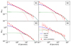 |
Fig. A.1. Auto-correlation data points (in red) and the best fit to the model (blue solid line) for the four redshift bins. The red dotted line and the green dashed line show the one-halo and two-halo terms, respectively. |
Prior distributions and results in each redshift bin for the parameters studied in the auto-correlation run.
Appendix B: Corner plots and tables
In this section we present the 1D and 2D posterior distributions as well as the priors and the results for the MCMC tomographic runs discussed in this work for the CCF case: the astrophysical only case with fixed cosmology to Planck (Fig. B.1 and Table B.1) and the astrophysical and cosmological cases (ΛCDM in Fig. B.2 and Table B.2, ω0CDM in Fig. B.3 and Table B.3 and ω0ωaCDM in Fig. B.4 and Table B.4). Moreover, Fig. B.5 and Table B.5 show the case where the cosmology is fixed to the Planck values, and Fig. B.6 and Table B.6 the case where the cosmology is fixed to the Planck values, except for h (which is the value provided by Riess et al. (2019)).
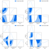 |
Fig. B.1. Corner plots for the fixed cosmology case, the cosmology being fixed to the Planck value. The posteriors distributions in Bin1, Bin2, Bin3, and Bin4 are shown from left to right, top to bottom. The contours are set to 39.3% and 86.5% |
Priors and results for the fixed cosmology case using the Planck values.
Priors and results for the ΛCDM case, with the astrophysical parameters and ΩM, σ8, and h set as free parameters.
Priors and results for the ω0CDM case and ωa fixed to zero.
Priors and results for the MCMC run on the astrophysical parameters and the cosmological parameters: ΩM, σ8, h, ω0, and ωa.
Priors and results for the MCMC run on astrophysical parameters and the cosmological ω0.
Priors and results for the MCMC run on astrophysical parameters and the cosmological ω0, with the h fixed to Riess et al. (2019).
The relevant 1σ and 2σ levels for a 2D histogram of samples is 39.3% and 86.5%, not 68% and 95%. Otherwise, there is no direct comparison with the 1D histograms above the contours. For visualisation purposes, each panel of Figs. B.2, B.3, and B.4 shows the astrophysical parameters posterior distribution in each bin, together with the cosmological parameters. The cosmological parameters posterior distributions are the same in all panels as the fit is performed jointly on the four redshift bins.
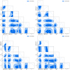 |
Fig. B.2. Corner plots for the ΛCDM case, with the astrophysical parameters and ΩM, σ8, and h set as free parameters; the rest of the cosmological parameters are fixed to the Planck values. The posteriors distributions in Bin1, Bin2, Bin3, and Bin4 are shown from left to right, top to bottom. The contours are set to 39.3% and 86.5%. |
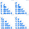 |
Fig. B.3. Corner plots for the ω0CDM case, where the rest of the cosmological parameters are fixed to the Planck values. The posteriors distributions in Bin1, Bin2, Bin3, and Bin4 are shown from left to right, top to bottom. The contours are set to 39.3% and 86.5%. |
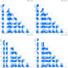 |
Fig. B.4. Corner plots for the flat prior case on the astrophysical parameters and ΩM, σ8, h, ω0, and ωa cosmological parameters. The posteriors distributions in Bin1, Bin2, Bin3, and Bin4 are shown from left to right, top to bottom. The contours are set to 0.393% and 0.865%. |
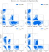 |
Fig. B.5. Corner plots for the flat prior case on the astrophysical and ω0 parameters with h fixed to the Planck value. The posterior distributions in Bin1, Bin2, Bin3, and Bin4 are shown from left to right, top to bottom. The contours are set to 3.93% and 86.5%. |
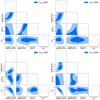 |
Fig. B.6. Corner plots for the flat prior case on the astrophysical and ω0 parameters with h fixed to the Riess value. The posterior distributions in Bin1, Bin2, Bin3, and Bin4 are shown from left to right, top to bottom. The contours are set to 39.3% and 8.65%. |
The columns in the tables are, from left to right: the bin to which the astrophysical parameters refer and the cosmological case when present, the names of the parameters, the priors choice for the run and the mean, median, 68% confidence intervals (C.I.), and the peak of the posterior distributions. The > and < signs in the C.I. column refer to lower and upper limits, respectively.
All Tables
Prior distributions and results in each redshift bin for the parameters studied in the auto-correlation run.
Priors and results for the ΛCDM case, with the astrophysical parameters and ΩM, σ8, and h set as free parameters.
Priors and results for the MCMC run on the astrophysical parameters and the cosmological parameters: ΩM, σ8, h, ω0, and ωa.
Priors and results for the MCMC run on astrophysical parameters and the cosmological ω0.
Priors and results for the MCMC run on astrophysical parameters and the cosmological ω0, with the h fixed to Riess et al. (2019).
All Figures
|
Fig. 1. Normalised redshift distribution of the background (red line) and foreground (blue line) samples. The coloured areas represents the selected ranges of redshift: in red the 1.2 < z < 4.0 interval for the background SMGs sample and in different shades of blue the 0.1 < z < 0.2, 0.2 < z < 0.3, 0.3 < z < 0.5, and 0.5 < z < 0.8 bins for the foreground GAMA galaxies. |
| In the text | |
|
Fig. 2. CCF data computed on Herschel SMGs (as background sample) and GAMA galaxies (as lenses sample) in the mini-Tiles data sets (red points) for the different redshift bins (from left to right, top to bottom): 0.1–0.2 (Bin1), 0.2–0.3 (Bin2), 0.3–0.5 (Bin3), and 0.5–0.8 (Bin4). The empty circles are the data discarded from the MCMC analysis, as explained in the text. The best fits performed in this work are also shown: the runs allowing for astrophysical parameters only (solid line) and for astrophysical and cosmological parameters: σ8, ΩM, and h (dotted line); σ8, ΩM, h, and ω0 (dashed line); and σ8, ΩM, h, ω0, and ωa (dash-dotted line). In the left panel the peaks of the marginalised 1D posterior distributions are used, and in the right panel the mean is used. |
| In the text | |
|
Fig. 3. One-dimensional posterior distributions of the HOD parameters log(Mmin/M⊙), log(M1/M⊙), and α (from left to right) in each redshift bin for the auto-correlation run. Results for Bins 1–4 are depicted as black solid, red dashed, blue dotted, and green dash-dotted lines, respectively. |
| In the text | |
|
Fig. 4. One-dimensional posterior distributions of the HOD parameters log(Mmin/M⊙), log(M1/M⊙) and α (from left to right) in each redshift bin for the CCF run with a fixed cosmology. Results for Bins 1–4 are depicted as black solid, red dashed, blue dotted and green dash-dotted lines, respectively. |
| In the text | |
|
Fig. 5. One-dimensional posterior distributions for log(Mmin/M⊙) (first column) and log(M1/M⊙) (second column) in Bins 1, 2, 3, and 4 (from top to bottom, respectively) for the run on just the HOD parameters (black solid lines) and for the three runs on the astrophysical and cosmological parameters jointly, namely within ΛCDM (red dashed lines), within ω0CDM (blue dotted lines), and within ω0ωaCDM (green dash-dotted lines). |
| In the text | |
|
Fig. 6. One-dimensional posterior distributions of ΩM, σ8, and h (from left to right) for the results in Bonavera et al. (2020) (black solid lines), and for the three MCMC runs performed jointly on the astrophysical and cosmological parameter in this work, namely within ΛCDM (red dashed lines), within ω0CDM (blue dotted lines), and within ω0ωaCDM (green dash-dotted lines). |
| In the text | |
|
Fig. 7. Contour plot of the two-dimensional posterior distribution of ΩM and σ8 for the three MCMC runs where the astrophysical and cosmological parameters are jointly analysed, namely within ΛCDM (in green), within ω0CDM (in red), and within ω0ωaCDM (in blue). Moreover, in order to compare with previous results, those by Bonavera et al. (2020) are shown in black. The contours are set to 0.393 and 0.865. |
| In the text | |
|
Fig. 8. Contour plot of the two-dimensional posterior distribution of h and ω0 for the three MCMC runs where the astrophysical and cosmological parameters are jointly analysed, namely within ΛCDM (in green), the within ω0CDM (in red), and within ω0ωaCDM (in blue). The contours are set to 0.393 and 0.865. |
| In the text | |
|
Fig. 9. Contour plot of the two-dimensional posterior distribution of ω0 and ωa for the MCMC run within ω0ωaCDM. The contours are set to 0.393 and 0.865. |
| In the text | |
|
Fig. 10. Comparison among the contour plots in the ΩM – σ8 plane from Planck CMB lensing (blue), CFHTLenS (cyan), KV450 (grey), DES (magenta), and HSC (yellow) and the results from this work (green). Differently from the other 2D plots in this work, the contours here are set to 0.68 and 0.95. |
| In the text | |
|
Fig. 11. Comparison of ω0 results of this work at 68% C.I. (ω0CDM model in red and ω0ωaCDM model in yellow) with findings from some other experiments: DES (magenta), Planck_1 (baseline base_w_wa_plikHM_TT_lowl_lowE_BAO, cyan), Planck_2 (baseline base_w_plikHM_TT_lowl_lowE, blue), supernovae (purple), x-ray measurements (green). |
| In the text | |
|
Fig. A.1. Auto-correlation data points (in red) and the best fit to the model (blue solid line) for the four redshift bins. The red dotted line and the green dashed line show the one-halo and two-halo terms, respectively. |
| In the text | |
|
Fig. B.1. Corner plots for the fixed cosmology case, the cosmology being fixed to the Planck value. The posteriors distributions in Bin1, Bin2, Bin3, and Bin4 are shown from left to right, top to bottom. The contours are set to 39.3% and 86.5% |
| In the text | |
|
Fig. B.2. Corner plots for the ΛCDM case, with the astrophysical parameters and ΩM, σ8, and h set as free parameters; the rest of the cosmological parameters are fixed to the Planck values. The posteriors distributions in Bin1, Bin2, Bin3, and Bin4 are shown from left to right, top to bottom. The contours are set to 39.3% and 86.5%. |
| In the text | |
|
Fig. B.3. Corner plots for the ω0CDM case, where the rest of the cosmological parameters are fixed to the Planck values. The posteriors distributions in Bin1, Bin2, Bin3, and Bin4 are shown from left to right, top to bottom. The contours are set to 39.3% and 86.5%. |
| In the text | |
|
Fig. B.4. Corner plots for the flat prior case on the astrophysical parameters and ΩM, σ8, h, ω0, and ωa cosmological parameters. The posteriors distributions in Bin1, Bin2, Bin3, and Bin4 are shown from left to right, top to bottom. The contours are set to 0.393% and 0.865%. |
| In the text | |
|
Fig. B.5. Corner plots for the flat prior case on the astrophysical and ω0 parameters with h fixed to the Planck value. The posterior distributions in Bin1, Bin2, Bin3, and Bin4 are shown from left to right, top to bottom. The contours are set to 3.93% and 86.5%. |
| In the text | |
|
Fig. B.6. Corner plots for the flat prior case on the astrophysical and ω0 parameters with h fixed to the Riess value. The posterior distributions in Bin1, Bin2, Bin3, and Bin4 are shown from left to right, top to bottom. The contours are set to 39.3% and 8.65%. |
| In the text | |
Current usage metrics show cumulative count of Article Views (full-text article views including HTML views, PDF and ePub downloads, according to the available data) and Abstracts Views on Vision4Press platform.
Data correspond to usage on the plateform after 2015. The current usage metrics is available 48-96 hours after online publication and is updated daily on week days.
Initial download of the metrics may take a while.