| Issue |
A&A
Volume 656, December 2021
|
|
|---|---|---|
| Article Number | A143 | |
| Number of page(s) | 15 | |
| Section | Numerical methods and codes | |
| DOI | https://doi.org/10.1051/0004-6361/202141454 | |
| Published online | 15 December 2021 | |
Ray-tracing in relativistic jet simulations: A polarimetric study of magnetic field morphology and electron scaling relations
Max-Planck-Institut für Radioastronomie, Auf dem Hügel 69, 53121 Bonn, Germany
e-mail: This email address is being protected from spambots. You need JavaScript enabled to view it.
Received:
2
June
2021
Accepted:
4
September
2021
Abstract
Context. The jets emanating from the centers of active galactic nuclei are among the most energetic objects in the Universe. Investigating how the morphology of the jet’s synchrotron emission depends on the magnetic nature of the jet’s relativistic plasma is fundamental to the comparison between numerical simulations of relativistic jets and their observed polarization.
Aims. Through the use of 3D relativistic magnetohydrodynamic jet simulations (computed using the PLUTO code) we study how the synchrotron emission from a jet depends on the morphology of its magnetic field structure. Through the application of polarized radiative transfer and ray-tracing (via the RADMC-3D code), we create synthetic radio maps of the total intensity of a jet as well as the linearly and circularly polarized intensity for each jet simulation.
Methods. In particular, we create synthetic ray-traced images of the polarized synchrotron emission from a jet when this latter carries a predominantly poloidal, helical, and toroidal magnetic field. We also explore several scaling relations in which the underlying electron power-law distribution is set proportional to: (i) the jet’s thermal plasma density, (ii) its internal energy density, and (iii) its magnetic energy density.
Results. We find that: (i) the jet emission is edge-brightened when the magnetic field is toroidal in nature and spine brightened when the magnetic field is poloidal in nature; (ii) the circularly polarized emission exhibits both negative and positive sign for the toroidal magnetic field morphology at an inclination of i = 45° as well as i = 5°; and (iii) the relativistic jet’s emission is largely independent of different emission scaling relations when the ambient medium is excluded.
Key words: galaxies: jets / magnetic fields / polarization / radiative transfer / relativistic processes / magnetohydrodynamics (MHD)
© J. A. Kramer and N. R. MacDonald 2021
 Open Access article, published by EDP Sciences, under the terms of the Creative Commons Attribution License (https://creativecommons.org/licenses/by/4.0), which permits unrestricted use, distribution, and reproduction in any medium, provided the original work is properly cited.
Open Access funding provided by Max Planck Society.
1. Introduction
Collimated supersonic flows of plasma are characteristic of many astrophysical objects. These phenomena are known as jets and emanate from compact systems (e.g., proto-stars) as well as from supermassive black holes (SMBHs). They are among the most energetic objects in the Universe and commonly emanate from the centers of active galaxies. The class of radio-loud active galactic nuclei (AGN) exhibit jet emission. These objects are mostly embedded in massive elliptical galaxies and only account for less than 10% of observed AGN. Launched from a central engine such as a SMBH, the jets can be accelerated to highly relativistic speeds and remain collimated up to kilo-parsec (kpc) scales. AGN emit radiation across the electromagnetic spectrum, and observations of the jet emission reveal a featureless power-law spectrum. Together with the high level of linear polarization (up to 60 − 70%), the physical process of synchrotron radiation can explain the emission as well as the optical flux (Troja et al. 2017). From the radio emission, the presence of a magnetic field can be inferred and is commonly thought to play a key role in the launching and collimation process of the jet. AGN jets can extend to hundreds of kiloparsecs even though the jet-launching region occurs on scales of a few gravitational radii from the black hole (BH). On larger scales, jets are thought to be kinetically dominated and therefore contain relatively weak magnetic fields. However, within the collimation region, jets are thought to be magnetically dominated. Theoretical studies of jet formation suggest that strong magnetic fields are an essential mechanism for launching jets (Blandford & Znajek 1977). One of the main conclusions of a number of relativistic jet simulations is that the jet transitions from being magnetically dominated to kinetically dominated as it propagates (e.g., Martí et al. 1997).
Very-long-baseline interferometric (VLBI) imaging of the synchrotron emission emanating from jets commonly reveals a bright central feature (referred to as the radio core) and a series of components that separate from the core over time (i.e., blobs or plasmoids). There are also (in some sources) features downstream of the core that, in contrast to the plasmoids, appear to be stationary relative to the radio core (e.g., Ojha et al. 2010; Fromm et al. 2013). These standing features within the jet are commonly interpreted as recollimation shocks within the jet flow (Daly & Marscher 1988).
A continuum approximation of the plasma nature of the jet (i.e., relativistic magnetohydrodynamics – RMHD) can be implemented based on the assumption that the jet radius, Rj, is much larger than the Debye-Length1 and gyroradius2 of the jet’s plasma (Hawley et al. 2015). Theoretical models of AGN jets have lead authors to postulate that the jet plasma is likely magnetized with a large-scale helical morphology related to the launching of the jet by the rotation of the central black hole and accretion disk (Blandford & Znajek 1977; Blandford & Payne 1982; Hardee et al. 2007). Recent observational evidence indicates that a large fraction of parsec-scale jets do indeed exhibit polarization signatures of helical magnetic field components. This is based on the detection of statistically significant transverse Faraday rotation measure (RM) gradients across the jet on parsec scales (Gabuzda et al. 2008).
The presence of a helical/toroidal magnetic field within the jet can (in theory) produce current-driven instabilities within the jet flow (Kadowaki et al. 2021). These instabilities can then produce sites of magnetic reconnection within the jet plasma which in turn can result in particle acceleration (Singh et al. 2016; Striani et al. 2016). Recent particle-in-cell (PIC) simulations (e.g., Sironi et al. 2021) have indeed shown that magnetic reconnection events within relativistically jetted plasma can efficiently generate power-law distributions of electrons (see also, Sironi & Spitkovsky 2014; Guo et al. 2015; Werner et al. 2016; Guo et al. 2019; Matthews et al. 2020). However, many of these PIC calculations lack sufficient grid sizes to model the length scales of astrophysical jets.
In the present paper, we set about carrying out a systematic study of how the fractional levels and morphology of both linearly and circularly polarized synchrotron emission depend on the underlying magnetic field morphology of the jet as well as various fluid scalings for the underlying electron power-law distribution. This study is executed with fully 3D relativistic magnetohydrodynamic jet simulations coupled with full Stokes polarized radiative transfer via ray-tracing.
RMHD simulations are unable to reproduce the kinetic-scale physics of the jet (i.e., self-consistently generating the non-thermal distribution of electrons responsible for the observed synchrotron emission). We therefore rely on a purely macroscopic model of the jet that simulates the large-scale dynamics of the thermal plasma within the jet flow. We explore various emission recipes for mapping from the thermal fluid variables to the non-thermal distribution of electrons (see, e.g., Porth et al. 2011). This mapping is carried out as a post-process step. In particular, we apply three scaling relations in which the non-thermal distribution of electrons is assumed to be proportional to the (i) density, (ii) thermal pressure, and (iii) magnetic energy density of the plasma. We also examine the effect that different magnetic field morphologies within the jet (namely; poloidal, helical, and toroidal) have on the dynamics of the jet as well as the resultant polarized emission.
Our current jet simulations, while applicable to parsec-scale jets, lack sufficient micro physics (such as magnetic reconnection) to self-consistently generate power-law distributions of electrons. However, our emission calculations provide: (i) an important bridge between the micro physical scales of reconnecting current sheets and parsec-scale jets, and (ii) a valuable point of comparison for the next generation of synthetic synchrotron emission maps to be produced via hybrid fluid particle schemes (see, e.g., Vaidya et al. 2018).
This paper is structured as follows: Sect. 2 gives an introduction to the principles of relativistic magnetohydrodynamics and polarized radiative transfer and introduces the PLUTO (Mignone et al. 2007) and RADMC-3D (Dullemond et al. 2012) codes. We perform a full Stokes analysis with an emphasis on studying the jet’s circularly polarized synchrotron emission. For this, the dependence of the jet’s polarization on the magnetic field morphology, that is, poloidal, helical, and toroidal, is investigated in Sect. 3. In Sect. 4 we explore the effect that different thermal-fluid-to -non-thermal-electron-emission scaling relations have on the resulting jet emission. Section 5 outlines different numerical approaches, that is, when no jet tracer is included or the lower energy cutoff is computed differently. In Sect. 6 we compare our numerical results to recent observations of jets. Finally, our conclusions are summarized in Sect. 7.
2. Numerical methods
2.1. Principles of the relativistic magnetohydrodynamics in the PLUTO code
To model magnetized fluid flows, the PLUTO code integrates a system of conservation laws which can be expressed in general as:
 (1)
(1)
where Uk is a state vector of k conservative quantities and Tik is a rank 2 tensor. Moreover, ∂i is the four-gradient. The explicit form depends on the physical module selected within the code.
PLUTO solves a time-dependent nonlinear system of special relativistic conservation laws, which in general have the form of Eq. (1). To account for the motion of an ideal relativistic magnetized fluid, that is, in relativistic magnetohydrodynamics, mass and energy-momentum are conserved. The solution to the specified problem of relativistic magnetohydrodynamics and therefore the conservative variables and respective fluxes for RMHD are expressed as:
 (2)
(2)
where v = (vx,vy,vz)T is the fluid’s velocity,  (j ∈ {x, y, z}) is the unit vector in the direction of the ith axis of a 3D Cartesian coordinate system, and bi are the spatial components of the covariant magnetic field vector. The quantities in Eq. (2) are defined as follows: (Mignone & Bodo 2006):
 (3)
(3)
Hence, the components of Uk resulting from the conservation laws are the laboratory density D, the three components of both momentum m and magnetic field B, and the total energy density E, respectively.
For a proper solution of Eq. (1) an additional equation of state (EoS) is specified that defines the specific enthalpy (see Mignone et al. 2005):
 (4)
(4)
which approximates a single-special-relativistic perfect gas. Here, Θ is the ratio of pressure to density, i.e., Θ = p/ρ.
2.2. Scaling
The PLUTO simulations are computed in dimensionless grid units, and therefore the thermal quantities of the RMHD jet flow must be properly scaled into physical units as a post process step. Computing dimensionless quantities has the advantage of avoiding either extremely small or large numbers at run time. A physical scaling is necessary whenever specific scales of length, time, and energy are included in the problem. The physical scaling of our RMHD jet simulations requires the definition of three fundamental units3:
![Mathematical equation: $$ \begin{aligned}&\mathrm{unit\,density} \quad \rho _0\, [\mathrm{g\,cm}^{-3}]\nonumber \\&\mathrm{unit\,length}\,\, \quad L_0\, [\mathrm{cm}]\nonumber \\&\mathrm{unit\,velocity} \quad { v}_0\, [\mathrm{cm\,s}^{-1}]. \end{aligned} $$](/articles/aa/full_html/2021/12/aa41454-21/aa41454-21-eq6.gif) (5)
(5)
From these unit values, other quantities such as the timescale of the code t0[s] can be computed: t0 = LO/v0. Similarly, the pressure and magnetic field scale factors can be computed from these unit values:  and
and  . To then scale the dimensionless fluid variables into cgs units we apply the scale factors:
 (6)
(6)
where ρ, p, and B are dimensionless grid values. For the simulations presented in this work we specify the following unit values: ρ0 ≃ 1.67 × 10⁻²² g cm−3, L0 ≃ 1.23 × 1016 cm, and v0 ≃ 3.0 × 1010 cm s−1. With this choice of values, the magnetic field strength along the jet will be of the order of gauss (G) to mG.
2.3. Mapping the non-thermal onto the thermal
An additional scaling relation is required in order to model the resultant non-thermal jet emission from our numerical simulations. The non-thermal quantities (i.e., electron number density and power-law energy cutoff) are inferred from the scaled thermal fluid variables of the simulation (i.e., plasma density, pressure, and magnetic field). This thermal to non-thermal mapping of our 3D RMHD jet simulations is used in the calculation of synchrotron emission maps. In particular, we initially assume an energy distribution of non-thermal relativistic electrons (NTEs) ne which follows a global power-law distribution. This approach is justified by observations as well as theoretical expectations for particle acceleration within jets. In particular, we adopt a power-law distribution in electron energy γ (where E = γmec2):
 (7)
(7)
where ne(γ) is the differential number of NTEs and γmin, γmax are the power-law cutoffs. The term n0 is a normalization constant, and the power-law index s is related to the spectral index α = (s − 1)/2.
To solve for the unknowns of the electron power-law (γmin and n0), see Eq. (7), we map the total number density of non-thermal electrons (NTEs) onto the thermal fluid variables (similar to Fromm et al. 2016). First, we assume the number density of the injected NTEs is proportional to the thermal fluid number density ρ:
 (8)
(8)
where ζe is the ratio of non-thermal to thermal particles (see Mimica 2012). Second, we assume that the total energy density of the NTEs is proportional to the thermal pressure p. Here, we connect the fluid’s pressure to the fluid’s internal energy density ϵ via the equation of state  , where
  is the adiabatic index. Consequently, the energy density becomes proportional to the internal energy density:
 (9)
(9)
where ϵe is the ratio between the energy stored in non-thermal particles to that stored in thermal particles. We set the thermal-to-non-thermal conversion factors to ζe = 1.0 and ϵe = 0.5.
Assuming that γmax ≫ γmin and s > 2 (we set s = 2.3), we solve this system of two equations (Eqs. (8) and (9)) for two unknowns (γmin and n0), which yields:
 (10)
(10)
2.4. Polarized radiative transfer and ray-tracing via RADMC-3D
For our ray-tracing calculations, we use the code RADMC-3D, which is a well-tested and documented ray-tracing software for computing astrophysical radiative transfer in 3D geometries. Our ray-tracing calculations are carried out in Cartesian coordinates and in the co-moving frame of the plasma after which the resultant fluxes are Doppler boosted to obtain the jet flux in the observer’s frame. The code reads in PLUTO output files that have been scaled into physical units (namely; the 3D distributions of B, ne, and γmin). RADMC-3D produces 2D Fits images containing full Stokes polarization maps. The radiative transfer is implemented in our plasma simulations through the use of transport coefficients for synchrotron absorption (κI,κQ,κU,κV), synchrotron emissivity (ηI,ηQ,ηU,ηV), Faraday rotation ( ), and Faraday conversion (
 and
and  ). Along individual rays our modified version of RADMC-3D solves the following transfer matrix:
 (11)
(11)
to obtain linear and circular polarization as a function of optical depth, i.e., dτ = κIdl. The code applies an analytical solution to Eq. (11) presented in Jones & Odell (1977) and summarized in MacDonald & Marscher (2018). The analytical solution is a function of the normalization constant n0, the low-energy cutoff γmin of the power-law distribution in Eq. (7), the strength of the magnetic field, and its orientation to our line of sight.
3. Magnetic field morphology study
3.1. Magnetic field prescriptions
Based on the physical scaling (presented in Sect. 2.2) and our NTE scaling relations (see Eq. (10)), we proceed to study the impact that different magnetic field morphologies within the jet (i.e., poloidal, toroidal, and helical) have on its polarized synchrotron emission. To produce different magnetic field morphologies, we implement (in Cartesian coordinates) expressions for the poloidal and toroidal components of the jet’s magnetic field at the jet injection point (i.e., orifice) in our simulations. The jet is oriented along the z-axis in our ray-tracing calculations. The x and y components of the jet’s magnetic field’s toroidal component are given by Nishikawa et al. (2019):
 (12)
(12)
where (xc,yc) is the location of the center of the jet, which in our simulation is set to (0, 0). The variable r defines the jet’s radius while a represents a magnetization radius. The parametrization constant of the magnetic field (bm) is given by:
 (13)
(13)
where σϕ is the magnetization parameter for the toroidal component. The constant poloidal term Bz threading the jet is written as:
 (14)
(14)
where σz is the magnetization parameter of the poloidal component. We choose σz = 1 for a purely poloidal magnetic field and σϕ = 1 for a purely toroidal field (Nishikawa et al. 2019; Mignone et al. 2009). A helical field is produced by setting σz = σϕ = 0.5. In Eq. (14) the variable pj is the jet pressure. In particular, pj is determined from our simulated jet Mach number M = 2.7 and bulk Lorentz factor Γ = 7 (i.e.,  ), where ρj is the jet density. The sum of both magnetization parameters is set to 1 to enforce an equipartition between the magnetic pressure and thermal pressure within the jet plasma. We point out that the magnetization radius a is equal to the jet radius
  as it reaches its maximum value.
Figure 1 illustrates the three different simulated magnetic field morphologies within the jet (from top to bottom: poloidal, helical, toroidal). Here, the poloidal magnetic field vectors are streaming along the jet in the z-direction while the vectors for the toroidal components are predominantly perpendicular to the jet axis. The helical magnetic field vectors are rotated about ∼45° in the jet’s direction. Two-dimensional slices through the jet are included in Appendix A and illustrate how the injected field morphologies persist down the jet axis.
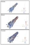 |
Fig. 1. Illustration of the three different magnetic field morphologies within the 3D RMHD jet simulations. The jet is streaming in the z-direction. The vectors represent the magnetic field strength (and orientation) in gauss (see the color bar) within each computational cell. From top to bottom: poloidal, helical, and toroidal magnetic field morphologies. |
3.2. Results
Figure 2 presents a summary of the various steps in our synthetic imaging pipeline. In particular, we are interested in studying the polarized properties of the jet’s recollimation shock. We image an intermediate epoch of each jet simulation, that is, when the jet’s hot spot or terminal shock has not yet propagated off the grid. Through the use of a jet tracer, we extract the region of plasma around the standing shock (demarcated with a purple box in the first panel of Fig. 2) in order to yield an unobscured view of the jet’s central spine, thus allowing us to focus on the jet flow upstream of the termination shock. These initial images were created using the poloidal magnetic field simulation. Panel a in Fig. 2 shows a 2D slice through the 3D jet simulation and displays the jet’s density in dimensionless grid units. Panels b and c illustrate the zoomed-in ray-traced total intensity maps of the resulting synchrotron emission when the jet is resolved without and with the use of a jet tracer to exclude the ambient medium, respectively. The jet is viewed at an angle to the jet-axis of i = 45° and propagates from top to bottom. In the absence of radiative cooling (i.e., synchrotron losses) and larger simulation sizes, we remove the bow shock from our ray-tracing calculations arbitrarily. Panel d displays the same snap-shot but rotated to a viewing angle of i = 5°. Finally, panel e is convolved with a Gaussian beam in order to indicate the resolution of the Global Millimeter VLBI Array (GMVA), and with an added Gaussian noise level (to mimic array sensitivity) of 10−1 Jy beam−1. These final images show a bright radio core associated with the standing shock in our simulations. In all our RMHD jet simulations (in which each computational box consists of 320 × 320 × 400 zones), we choose to view the source at a luminosity distance of 100 Mpc. The individual scaled cell size is 0.004 pc. All images in this paper are generated at an observing frequency of νobs = 86 GHz.
 |
Fig. 2. From left to right: a demonstration of our synthetic imaging pipeline: Panel a: starts with a 2D cut through our 3D RMHD jet colored by thermal density. Panels b–e: zoomed into an unobscured region of the jet’s standing shock (demarcated with a purple box in panel a) and show: (b) the ray-traced synchrotron emission without the use of a jet tracer; (c) the ray-traced synchrotron emission with the use of a jet tracer to exclude the ambient medium; (d) the same simulation epoch but rotated to a viewing angle of i = 5°; and (e) the ray-traced image convolved with a Gaussian beam indicative of the resolution of the GMVA and with a Gaussian noise floor (to mimic array sensitivity) of 10−1 Jy beam−1. |
We visualize the polarized synchrotron emission of the jet for three different magnetic field morphologies, that is, purely poloidal, helical, and purely toroidal. To begin with, the images in Fig. 3 show the total intensity of the jet’s emission in the left column, the linearly polarized intensity ( ) including electric vector position angles (EVPAs = 0.5arctan[U/Q]) in the middle column, and the circular polarization in the right column. Moreover, the different rows represent the three magnetic field morphologies introduced in Sect. 3.1. The top row depicts the poloidal magnetic field, the middle row the helical field, and the bottom row the purely toroidal magnetic field. All ray-traced images are viewed at 45° to the jet-axis in Fig. 3.
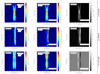 |
Fig. 3. Ray-traced images of our jet propagating from top to bottom in total intensity (left column), in linearly polarized intensity (middle column), and circular polarization (right column). The pictures illustrate similar epochs in the jet’s evolution during each 3D RMHD simulation at 86 GHz. The jet carries a purely poloidal magnetic field (top row), a helical magnetic field (middle row), and a purely toroidal magnetic field (bottom row). Integrated values of the fractional linear and circular polarization are listed to the lower right in the middle and right columns. The purely toroidal field jet appears edge-brightened in contrast to the poloidal jet which is brightest along the spine. |
We can see that the emission for the purely poloidal magnetic field is concentrated in the inner part of the jet, and is brightest within the standing recollimation shock. The EVPAs, shown as white line segments in the middle column of Fig. 3, are predominantly perpendicular to the magnetic field orientation, in the ideal case. As the poloidal field is streaming in the direction of the jet, the EVPAs accurately convey the field orientation within our simulations. In addition, the circular polarization has only positive values, unlike the purely toroidal magnetic field.
The toroidal magnetic field (bottom row of Fig. 3) clearly produces emission that is centered along the edges of the jet, as we see an edge-brightened jet in all our images along the bottom row. In addition, we can see both positive and negative circular polarization highlighting the changing orientation of the jet’s magnetic field with respect to our line of sight.
The helical magnetic field illustrated in the middle row in Fig. 3 exhibits a mixture of the emission and polarization morphologies present in the toroidal and poloidal cases. The emission is concentrated on the right side of the relativistic jet which stresses the structure of the helical magnetic field lines.
Additionally, we compute integrated levels of fractional polarization. These are flux-weighted averages of the Stokes parameters across the entire jet emission region in each set of images (listed to the lower right in the linearly polarized and circularly polarized images of Fig. 3,  and
and  ). The fractional linear polarization decreases from the poloidal to the toroidal magnetic field model (from ∼7.1% to ∼1.8%) and drops for the helical magnetic field morphology (∼1.6%). The fractional circular polarization also decreases from the poloidal to the helical magnetic field structure. The calculated value for the toroidal field jet changed sign and is several orders of magnitude smaller (from ∼ − 4.8 × 10⁻¹% to ∼1.2 × 10⁻⁵%).
The images presented in Fig. 3 display a resolved RMHD jet observed at 45°. To further simulate the emission of a blazar radio core we: (i) alter the viewing angle to 5°, (ii) convolve our resultant images with a Gaussian beam indicative of the resolution of the GMVA, and (iii) mimic VLBI array sensitivity by introducing a Gaussian noise floor of 10−4 Jy beam−1. This results in a dynamic range of ∼1 : 100 000 in our synthetic images. Figure 4 shows the total intensity of the jet’s emission in the left column, the linearly polarized intensity including EVPAs in the middle column, and the circular polarization in the right column. Again, the different rows represent the three magnetic field morphologies. The top row depicts purely poloidal magnetic field, the middle one the helical field, and the bottom one the purely toroidal magnetic field. All simulations are viewed edge-on to the jet axis in Fig. 4.
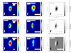 |
Fig. 4. Ray-traced images of RMHD jet simulations in total intensity (left), linearly polarized intensity (middle), and circular polarization (right) when each jet is viewed edge-on to the jet axis. The images highlight similar epochs in the jet’s evolution during each 3D RMHD simulation at 86 GHz. The jet carries a purely poloidal magnetic field (top row), a helical magnetic field (middle row), and a purely toroidal magnetic field (bottom row). The ray-traced images are convolved with a Gaussian beam indicative of the resolution of the GMVA and with a Gaussian noise floor of 10−4 Jy beam−1. |
In total intensity, the poloidal field case exhibits a bright central radio core, whereas in contrast the helical and toroidal field cases exhibit emission peaks offset from the central shock. Also, the helical and toroidal field cases exhibit two signs in circular polarization whereas the poloidal field case exhibits only one. In all cases, the linear polarized emission peaks are offset from the total intensity peaks which is commonly seen in blazars.
Again, we computed integrated levels of fractional linear and circular polarization ( and
and  , listed to the lower right in the linear polarization and circular polarization images of Fig. 4). In the case of i = 5° and in contrast to the calculated values at 45°, the fractional linear polarization increases from the poloidal to the helical and then to the toroidal magnetic field model (from ∼2.0% to ∼6.0%). The fractional circular polarization decreases and changes sign from the poloidal to toroidal magnetic field model (from ∼1.5% to ∼ − 3.8 × 10⁻²%). The fractional circular polarization peaks for the helical magnetic field at ∼2.7%.
Here, the most striking result is that Figs. 3 and 4 demonstrate that resolved circular polarization imaging of relativistic jets can potentially be used to distinguish between a purely poloidal and a purely toroidal magnetic field configuration within standing or recollimation shocks.
4. Emission recipe study
4.1. Emission recipe prescriptions
We now shift our focus to better understanding the impact that different electron scaling relations have on the synchrotron polarization produced in our RMHD jet simulations. In particular, we explore three additional scaling relations to account for the jet’s microphysics by adopting the methods presented in Porth et al. (2011). In particular, we set the NTEs energy distribution proportional to: (i) the fluid density, (ii) the thermal pressure, and (iii) the magnetic energy density:
 (15)
(15)
In this treatment, we set the conversion factors ζe = ϵe = ϵB = 1 (see Sect. 2.3), where ϵB is the equipartition fraction. Again, ne(γ) takes the form of a power-law, see Eq. (7).
Instead of solving the terms in Eq. (15) for two unknowns, we assume fixed bounds for the electron power-law (γmin and γmax). The lower cutoff for injected NTEs is set to γmin = 10 and the upper limit to γmax = 106 ⋅ γmin (see Eq. (7)). We solve each equation in Eq. (15) for n0 as a function of either p, ρ, or B:
 (16)
(16)
Again, we set the electron power-law index to s = 2.3 (hence α = 0.65).
4.2. Results
Based on the solutions presented in Eq. (16) we generate synthetic maps of total intensity, linearly polarized intensity, circular polarization, and calculate integrated fractional levels of polarization. Figure 5 presents resolved total intensity images computed using the three emission recipes (see Eq. (15)). The top row illustrates the poloidal magnetic field, the middle row illustrates the helical field, and the bottom row illustrates the toroidal magnetic field. Here, we analyze the dependence on the electron scaling relations while viewing the jet at i = 45°. The left column shows images produced using the density scaling relation, the middle column shows images produced using the pressure scaling relation, and the right column shows images produced using the magnetic energy density scaling relation. We see that the three different scaling relations do not have a drastic impact on the resultant jet emission when using a jet tracer to exclude the ambient medium. Similar to our findings in Sect. 3.2, we see an edge-brightened jet in the toroidal field case and a spine- or shock-brightened jet in the poloidal field case for all three electron scaling relations. Figure 6 shows the corresponding linear polarization maps with EVPAs overplotted. The EVPA orientations are similar to the orientations illustrated in Sect. 3.2.
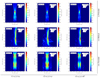 |
Fig. 5. Total intensity maps of our 3D RMHD jet simulations using different electron scaling relations. The jet is viewed at i = 45° and propagates from top to bottom in each frame. The images highlight similar epochs in the jet’s evolution of each 3D RMHD simulation at 86 GHz. From left to right: proportionality of the NTEs to the fluid’s density, internal energy density, and magnetic energy density. From top to bottom: purely poloidal magnetic field, helical magnetic field, and purely toroidal magnetic field. |
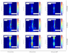 |
Fig. 6. Linearly polarized emission maps of our 3D RMHD jet simulations using different emission electron scaling relations. The jet is viewed at i = 45° and propagates from top to bottom in each frame. The images highlight similar epochs in the jet’s evolution during each 3D RMHD simulation at 86 GHz. From left to right: proportionality of the NTEs to the fluid’s density, internal energy density, and magnetic energy density. From top to bottom: purely poloidal magnetic field, helical magnetic field, and purely toroidal magnetic field. |
Figure 7 shows the resulting circular polarization maps of the RMHD jet simulations for the three different electron scaling relations. The arrangement is the same as in Fig. 5. All three magnetic field morphologies again show only minor differences. The polarized synchrotron emission is focused in the center of the jet, highlighting the recollimation shock. The helical magnetic field exhibits positive circular polarization on the right side of the jet. For the toroidal magnetic field, the circular polarized emission shows positive values on the left part of the jet and negative values on the right (i.e., left- and right-handed). This is a reflection of the pitch angle present in the helical field case.
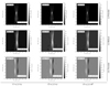 |
Fig. 7. Circular polarization maps of our 3D RMHD jet simulations using different emission electron scaling relations. The jet is viewed at i = 45° and propagates from top to bottom in each frame. The images highlight similar epochs in the jet’s evolution of each 3D RMHD simulation at 86 GHz. From left to right: proportionality of the NTEs to the fluid’s density, internal energy density, and magnetic energy density. From top to bottom: purely poloidal magnetic field, helical magnetic field, and purely toroidal magnetic field. |
Figures 8 through 10 show the same sequence of images for each scaling relation except that the jets are now viewed at an inclination of i = 5° to the jet axis. In particular, the proportionality to the thermal pressure, visible in the middle column of Fig. 9, highlights both the recollimation shock in the central region of the jet and the pressurized regions of the ambient plasma due to interactions with the surrounding medium.
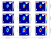 |
Fig. 8. Ray-tracing images of our jets in total intensity when each jet is viewed edge-on. The images highlight similar epochs in the jet’s evolution during each 3D RMHD simulation at 86 GHz. From left to right: proportionality of the NTEs to the fluid’s density, internal energy density, and magnetic energy density. From top to bottom: purely poloidal magnetic field, helical magnetic field, and purely toroidal magnetic field. The ray-traced images are convolved with a Gaussian beam indicative of the resolution of the GMVA and with a Gaussian noise floor of 10−4 Jy beam−1. |
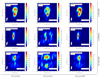 |
Fig. 9. Ray-tracing images of our jets in linearly polarized intensity when each jet is viewed edge-on. The images highlight similar epochs in the jet’s evolution during each 3D RMHD simulation at 86 GHz. From left to right: proportionality of the NTEs to the fluid’s density, internal energy density, and magnetic energy density. From top to bottom: purely poloidal magnetic field, helical magnetic field, and purely toroidal magnetic field. The ray-traced images are convolved with a Gaussian beam indicative of the resolution of the GMVA and with a Gaussian noise floor of 10−4 Jy beam−1. |
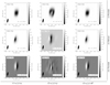 |
Fig. 10. Ray-tracing images of our jets in circular polarization when each jet is viewed edge-on. The images highlight similar epochs in the jet’s evolution during each 3D RMHD simulation at 86 GHz. From left to right: proportionality of the NTEs to the fluid’s density, internal energy density, and magnetic energy density. From top to bottom: purely poloidal magnetic field, helical magnetic field, and purely toroidal magnetic field. The ray-traced images are convolved with a Gaussian beam indicative of the resolution of the GMVA and with a Gaussian noise floor of 10−4 Jy beam−1. |
The integrated levels of fractional linear and fractional circular polarization (shown to the lower right in Figs. 6, 7, 9, and 10) exhibit the same level and behavior as discussed in Sect. 3.2 and show no major dependency on the chosen electron scaling relation.
5. Electron emission scaling-relation variations
There are two additional variations of the electron emission scaling relations presented in Sect. 4. In the first variation, we exclude the use of a jet tracer (which is a PLUTO variable) and consider the impact the toroidal magnetic field morphology and various emission scaling relations have on the ray-traced image when including the surrounding ambient medium. In a second variation, we keep the jet tracer but replace the assumption of a constant lower cutoff in the electron power-law spectrum and instead compute γmin as a function related to the thermal pressure and density.
5.1. No jet tracer
In contrast to Sect. 4.2, we no longer make use of a jet tracer to exclude the surrounding ambient medium in our ray-tracing images. Figure 11 highlights the resultant emission for the toroidal magnetic field case for the three electron scaling relations with the additional component of the ambient medium. For simplicity, we choose to show the total intensity where we see the most striking difference to the results presented in Sect. 4.2. As before, the left column shows images produced using the density scaling relation, the middle column shows images produced using the pressure scaling relation, and the right column shows images produced using the magnetic energy density scaling relation. In contrast to Sect. 4.2, we clearly see the impact of the various emission scaling relations on the jet emission when assuming a toroidal magnetic field morphology and including the ambient medium. The ambient medium is most visible for the density scaling relation and the jet structure itself is largely hidden behind the intervening ambient plasma (which is not radiatively cooled in our simulations). Clearly, the second two recipes (which are proportional to thermal pressure and magnetic energy density) are better at highlighting the jet through the intervening ambient plasma. A solution to the arbitrary use of a jet tracer, moving forward, will be to properly include the effects of synchrotron cooling and diffusive shock acceleration – this is planned for a future paper.
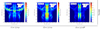 |
Fig. 11. Total intensity maps of our 3D RMHD jet simulations using different electron scaling relations and a purely toroidal magnetic field morphology. The images highlight similar epochs in the jet’s evolution during each 3D RMHD simulation at 86 GHz. The images, in contrast to Fig. 5, are generated without the use of a jet tracer and illustrate both the emission of the ambient medium and the hidden jet structure. The jet is viewed at i = 45° and propagates from top to bottom in each frame. From left to right: proportionality of the NTEs to the fluid’s density, internal energy density, and magnetic energy density. |
5.2. Lower cutoff for injected NTEs
In the second variation, we keep the jet tracer but instead compute the constant lower cutoff for injected NTEs (γmin = 10 for Sect. 4) with a prescription based on the ratio between thermal pressure and density (similar to Porth et al. 2011). In particular, we compute (cell-to-cell)
 (17)
(17)
Figure 12 shows the resulting jet emission in total intensity. The arrangement is the same as in Fig. 11. The proportionality to (i) the density, (ii) pressure, and (iii) magnetic energy density does not show any major differences when compared with the lower panels of Fig. 5 (in which we set γmin = 10). The jet remains edge-brightened for the toroidal magnetic field as seen in Sect. 4.2.
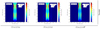 |
Fig. 12. Total intensity maps of our 3D RMHD jet simulations using different electron scaling relations and a purely toroidal magnetic field morphology. The images highlight similar epochs in the jet’s evolution during each 3D RMHD simulation at 86 GHz. The images are created with a jet tracer which excludes the obscuring ambient medium. The images are comparable to the lower panels of Fig. 5 in which, in contrast to computing γmin from the ratio of pressure to density, it is fixed to 10. The jet is viewed at i = 45° and propagates from top to bottom in each frame. From left to right: proportionality of the NTEs to the fluid’s density, internal energy density, and magnetic energy density. The jet structure does not show considerable differences although the jet is most edge-brightened for the most right proportionality. |
6. Discussion
A wealth of new polarimetric data has been amassed for relativistic jets over the last decade, namely maps of AGN in both linearly polarized intensity and circular polarization, maps of Faraday RM gradients along the jet, and analysis of EVPA orientation along the jet, all of which help to probe the underlying magnetic field geometry. In this section, we make further comparisons between our ray-traced emission maps and observations in order to better understand and interpret the different polarimetric features we observe in our simulations.
Faraday RM gradients observed transverse to the jet axis hint at the existence of helical magnetic fields (e.g., in 0133+479, see Gabuzda 2018; Gabuzda et al. 2018). In a future work, we plan to experiment with generating synthetic RM maps of our three jet simulations to explore the robustness of RM as a metric of the jet’s internal magnetic field structure.
Helical or toroidal magnetic field morphologies have been invoked to explain an increase in linear polarization towards the edges of the jet (Pushkarev et al. 2005; Lyutikov et al. 2005). This edge-brightened emission morphology is clearly seen in our simulations.
As discussed in Gabuzda (2018), a purely toroidal magnetic field should result in symmetric edge-brightened emission across the jet, whereas in contrast a helical magnetic field should result in asymmetric emission along the jet edges. These distinct emission morphologies are present within our simulations (see, e.g., Fig. 3).
In our poloidal field simulation the jet spine or shock dominates the emission. This emission morphology has been observed in the jet of NGC 1052 (Baczko 2020). In contrast, in the helical and toroidal field simulations the outer sheath is edge-brightened and dominates the emission. This emission morphology has been observed in the jet of 3C 84 (see, e.g., Giovannini et al. 2018; Kim et al. 2019; Paraschos et al. 2021).
Bi-modal EVPA patterns have been observed in a number of jets (O’Sullivan & Gabuzda 2009) in which the EVPAs preferentially align with the jet axis in the spine and, in contrast, appear predominantly perpendicular to the jet axis in the sheath. We see this bi-modal pattern in our toroidal field simulation (see, e.g., lower middle panel of Fig. 3).
The majority of blazars in which CP is detected tend to exhibit one sign/handedness of circular polarization (see, e.g., Homan & Lister 2006; Homan & Wardle 2004). However, a small number of sources exhibit both negative and positive CP in the radio core region (see, e.g., Vitrishchak et al. 2008). As illustrated in the right column of Fig. 4, we find that a poloidal field produces only one sign of CP in the radio core, whereas in contrast the toroidal field produces both signs of CP in the core. This highlights the potential of combining linear and circular polarization maps to make a more robust determination of the magnetic field orientation within the jet.
7. Conclusion
We carried out a systematic survey of full Stokes radiative transfer calculations, exploring the effects of (i) the jet’s magnetic field morphology and (ii) the various electron scaling relations on the resultant linear and circular polarized emission. Our findings can be summarized as follows.
-
Resolved circular polarization imaging has the potential to discriminate between a purely poloidal or a purely toroidal magnetic field morphology within the jet.
-
When the jet is resolved (i.e., Fig. 3), toroidal magnetic fields result in edge-brightened jets whereas poloidal magnetic fields seem to highlight the jet spine or recollimation shock.
-
The integrated levels of fractional linear
 and circular polarization
  are only mildly sensitive to the choice of electron scaling relation. However, the integrated fractional circular polarization of the toroidal jet is found to be several orders of magnitude smaller than the poloidal and helical jets.
 -
Scaling the electron number density to the thermal (fluid) density ρ, pressure p, or magnetic energy density B2 while fixing the bounds of the electron power-law distribution (γmin and γmax) does not seem to have an appreciable effect on the morphology of the linear and circular polarized emission within the shock when the ambient medium is excluded from the ray-tracing. However, when the ambient medium is included, the magnetic energy density recipe best highlights the jet emission through the intervening plasma.
In an effort to further compare simulations to observations, our numerical RMHD jet models have formed the basis of an accepted VLBA proposal to conduct deep full Stokes imaging of a number of blazar jets. This will allow us to make further comparisons between our numerical models and CP observations in an attempt to better understand the nature of the intrinsic magnetic field morphologies of relativistic jets. In the future, we plan to incorporate the effects of synchrotron cooling and diffusive shock acceleration in our ray-tracing calculations (see, e.g., Vaidya et al. 2018).
The Debye-Length is the length scale in a plasma over which the charge of a plasma is shielded by intervening electrons.
The gyroradius (also referred to as the Larmor radius) is the radius about which an electron rotates about a magnetic field line.
For further details see the PLUTO code (http://plutocode.ph.unito.it).
Acknowledgments
This research was supported through a PhD grant from the International Max Planck Research School (IMPRS) for Astronomy and Astrophysics at the Universities of Bonn and Cologne. The three-dimensional jet simulations presented in this paper are computed with the PLUTO code. The ray-tracing software RADMC-3D produced the polarized images of the synchrotron emission. The authors are grateful to E. Ros for feedback regarding VLBI, M. Perucho for helpful discussions on the physics of RMHD jet simulations, and to the referee, P. Hughes, for a thorough review of this manuscript.
References
- Baczko, A. K. 2020, PhD Thesis, Max-Planck-Institute for Radioastronomy, Germany [Google Scholar]
- Blandford, R. D., & Payne, D. G. 1982, MNRAS, 199, 883 [CrossRef] [Google Scholar]
- Blandford, R. D., & Znajek, R. L. 1977, MNRAS, 179, 433 [NASA ADS] [CrossRef] [Google Scholar]
- Daly, R. A., & Marscher, A. P. 1988, ApJ, 334, 539 [Google Scholar]
- Dullemond, C. P., Juhasz, A., Pohl, A., et al. 2012, Astrophysics Source Code Library [record ascl:1202.015] [Google Scholar]
- Fromm, C. M., Ros, E., Perucho, M., et al. 2013, A&A, 557, A105 [NASA ADS] [CrossRef] [EDP Sciences] [Google Scholar]
- Fromm, C. M., Perucho, M., Mimica, P., & Ros, E. 2016, A&A, 588, A101 [NASA ADS] [CrossRef] [EDP Sciences] [Google Scholar]
- Gabuzda, D. 2018, Galaxies, 6, 9 [NASA ADS] [CrossRef] [Google Scholar]
- Gabuzda, D. C. 2018, Proc. Int. Astron. Union, 14, 189 [NASA ADS] [CrossRef] [Google Scholar]
- Gabuzda, D. C., Vitrishchak, V. M., Mahmud, M., & O’Sullivan, S. 2008, ASP Conf. Ser., 386, 444 [NASA ADS] [Google Scholar]
- Gabuzda, D. C., Nagle, M., & Roche, N. 2018, A&A, 612, A67 [NASA ADS] [CrossRef] [EDP Sciences] [Google Scholar]
- Giovannini, G., Savolainen, T., Orienti, M., et al. 2018, Nat. Astron., 2, 472 [Google Scholar]
- Guo, F., Liu, Y.-H., Daughton, W., & Li, H. 2015, ApJ, 806, 167 [NASA ADS] [CrossRef] [Google Scholar]
- Guo, F., Li, X., Daughton, W., et al. 2019, ApJ, 879, L23 [Google Scholar]
- Hardee, P., Mizuno, Y., & Nishikawa, K.-I. 2007, Astrophys. Space Sci., 311, 281 [NASA ADS] [CrossRef] [Google Scholar]
- Hawley, J. F., Fendt, C., Hardcastle, M., Nokhrina, E., & Tchekhovskoy, A. 2015, Space Sci. Rev., 191, 441 [NASA ADS] [CrossRef] [Google Scholar]
- Homan, D. C., & Lister, M. L. 2006, AJ, 131, 1262 [NASA ADS] [CrossRef] [Google Scholar]
- Homan, D. C., & Wardle, J. F. C. 2004, ApJ, 602, L13 [CrossRef] [Google Scholar]
- Jones, T. W., & Odell, S. L. 1977, A&A, 61, 291 [NASA ADS] [Google Scholar]
- Kadowaki, L. H. S., de Gouveia Dal Pino, E. M., Medina-Torrejón, T. E., Mizuno, Y., & Kushwaha, P. 2021, ApJ, 912, 109 [NASA ADS] [CrossRef] [Google Scholar]
- Kim, J. Y., Krichbaum, T. P., Marscher, A. P., et al. 2019, A&A, 622, A196 [NASA ADS] [CrossRef] [EDP Sciences] [Google Scholar]
- Lyutikov, M., Pariev, V. I., & Gabuzda, D. C. 2005, MNRAS, 360, 869 [Google Scholar]
- MacDonald, N. R., & Marscher, A. P. 2018, ApJ, 862, 58 [CrossRef] [Google Scholar]
- Martí, J. M., Mueller, E., Font, J. A., Ibánez, J. M., & Marquina, A. 1997, ApJ, 479, 151 [CrossRef] [Google Scholar]
- Matthews, J. H., Bell, A. R., & Blundell, K. M. 2020, New Astron. Rev., 89, 101543 [CrossRef] [Google Scholar]
- Mignone, A., & Bodo, G. 2006, MNRAS, 368, 1040 [Google Scholar]
- Mignone, A., Plewa, T., & Bodo, G. 2005, ApJS, 160, 199 [CrossRef] [Google Scholar]
- Mignone, A., Bodo, G., Massaglia, S., et al. 2007, ApJS, 170, 228 [Google Scholar]
- Mignone, A., Ugliano, M., & Bodo, G. 2009, MNRAS, 393, 1141 [NASA ADS] [CrossRef] [Google Scholar]
- Mimica, P., Giannios, D., Metzger, B., & Aloy, M. A. 2012, EPJ Web Conf., 39, 04003 [NASA ADS] [CrossRef] [EDP Sciences] [Google Scholar]
- Nishikawa, K.-I., Mizuno, Y., Gómez, J., et al. 2019, Galaxies, 7, 29 [NASA ADS] [CrossRef] [Google Scholar]
- Ojha, R., Kadler, M., Boeck, M., et al. 2010, ArXiv e-prints [arXiv:1006.2097] [Google Scholar]
- O’Sullivan, S. P., & Gabuzda, D. C. 2009, MNRAS, 393, 429 [CrossRef] [Google Scholar]
- Paraschos, G. F., Kim, J. Y., Krichbaum, T. P., & Zensus, J. A. 2021, A&A, 650, L18 [NASA ADS] [CrossRef] [EDP Sciences] [Google Scholar]
- Porth, O., Fendt, C., Meliani, Z., & Vaidya, B. 2011, ApJ, 737, 42 [Google Scholar]
- Pushkarev, A. B., Gabuzda, D. C., Vetukhnovskaya, Y. N., & Yakimov, V. E. 2005, MNRAS, 356, 859 [Google Scholar]
- Singh, C. B., Mizuno, Y., & de Gouveia Dal Pino, E. M. 2016, ApJ, 824, 48 [NASA ADS] [CrossRef] [Google Scholar]
- Sironi, L., & Spitkovsky, A. 2014, ApJ, 783, L21 [NASA ADS] [CrossRef] [Google Scholar]
- Sironi, L., Rowan, M. E., & Narayan, R. 2021, ApJ, 907, L44 [CrossRef] [Google Scholar]
- Striani, E., Mignone, A., Vaidya, B., Bodo, G., & Ferrari, A. 2016, MNRAS, 462, 2970 [NASA ADS] [CrossRef] [Google Scholar]
- Troja, E., Lipunov, V. M., Mundell, C. G., et al. 2017, Nature, 547, 425 [NASA ADS] [CrossRef] [Google Scholar]
- Vaidya, B., Mignone, A., Bodo, G., Rossi, P., & Massaglia, S. 2018, ApJ, 865, 144 [Google Scholar]
- Vitrishchak, V. M., Gabuzda, D. C., Algaba, J. C., et al. 2008, MNRAS, 391, 124 [NASA ADS] [CrossRef] [Google Scholar]
- Werner, G. R., Uzdensky, D. A., Cerutti, B., Nalewajko, K., & Begelman, M. C. 2016, ApJ, 816, L8 [Google Scholar]
Appendix A: Persistence of the injected magnetic field morphology
The underlying magnetic field included in the RMHD jet simulations exhibits distinct characteristics for each simulation (i.e., poloidal, helical, toroidal). We implement a poloidal component (Bz, see Eq. 14) and toroidal components (Bx and By, see Eq. 12). The magnetization parameters (σz and σϕ - see Section 3.1) set the overall morphology of the field (i.e., by varying the ratio between the poloidal and toroidal components).
Figure A.1 illustrates how the magnetic field morphologies injected at the jet orifice persist down the jet. The left column shows 2D slices through the midplane of each simulation with the color scheme highlighting the component of the magnetic field (By) which is perpendicular to the jet axis. In contrast, the right column shows 2D slices through the jet’s midplane (see dashed line in left column), respectively, with the color scheme highlighting the component of the magnetic field (Bz) which is parallel to the jet direction. The upper, middle, and lower rows correspond to the poloidal, helical, and toroidal field simulations, respectively.
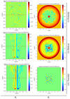 |
Fig. A.1. 2D slices through our 3D RMHD jets and are color coded according to the magnetic field component perpendicular to the jet axis – By (left column), and the field component parallel to the jet axis – Bz (right column) through the jet’s midplane (see dashed line in the left column). From top to bottom: Poloidal, helical, and toroidal magnetic field simulations. |
The slices presented in Fig. A.1 are made through the same simulation epochs used in our ray-tracing calculations above. Despite the existence of turbulent eddies and jet shear along each jet axis, the injected magnetic field morphologies largely persist down the jet (be it poloidal, helical, or toroidal).
All Figures
|
Fig. 1. Illustration of the three different magnetic field morphologies within the 3D RMHD jet simulations. The jet is streaming in the z-direction. The vectors represent the magnetic field strength (and orientation) in gauss (see the color bar) within each computational cell. From top to bottom: poloidal, helical, and toroidal magnetic field morphologies. |
| In the text | |
|
Fig. 2. From left to right: a demonstration of our synthetic imaging pipeline: Panel a: starts with a 2D cut through our 3D RMHD jet colored by thermal density. Panels b–e: zoomed into an unobscured region of the jet’s standing shock (demarcated with a purple box in panel a) and show: (b) the ray-traced synchrotron emission without the use of a jet tracer; (c) the ray-traced synchrotron emission with the use of a jet tracer to exclude the ambient medium; (d) the same simulation epoch but rotated to a viewing angle of i = 5°; and (e) the ray-traced image convolved with a Gaussian beam indicative of the resolution of the GMVA and with a Gaussian noise floor (to mimic array sensitivity) of 10−1 Jy beam−1. |
| In the text | |
|
Fig. 3. Ray-traced images of our jet propagating from top to bottom in total intensity (left column), in linearly polarized intensity (middle column), and circular polarization (right column). The pictures illustrate similar epochs in the jet’s evolution during each 3D RMHD simulation at 86 GHz. The jet carries a purely poloidal magnetic field (top row), a helical magnetic field (middle row), and a purely toroidal magnetic field (bottom row). Integrated values of the fractional linear and circular polarization are listed to the lower right in the middle and right columns. The purely toroidal field jet appears edge-brightened in contrast to the poloidal jet which is brightest along the spine. |
| In the text | |
|
Fig. 4. Ray-traced images of RMHD jet simulations in total intensity (left), linearly polarized intensity (middle), and circular polarization (right) when each jet is viewed edge-on to the jet axis. The images highlight similar epochs in the jet’s evolution during each 3D RMHD simulation at 86 GHz. The jet carries a purely poloidal magnetic field (top row), a helical magnetic field (middle row), and a purely toroidal magnetic field (bottom row). The ray-traced images are convolved with a Gaussian beam indicative of the resolution of the GMVA and with a Gaussian noise floor of 10−4 Jy beam−1. |
| In the text | |
|
Fig. 5. Total intensity maps of our 3D RMHD jet simulations using different electron scaling relations. The jet is viewed at i = 45° and propagates from top to bottom in each frame. The images highlight similar epochs in the jet’s evolution of each 3D RMHD simulation at 86 GHz. From left to right: proportionality of the NTEs to the fluid’s density, internal energy density, and magnetic energy density. From top to bottom: purely poloidal magnetic field, helical magnetic field, and purely toroidal magnetic field. |
| In the text | |
|
Fig. 6. Linearly polarized emission maps of our 3D RMHD jet simulations using different emission electron scaling relations. The jet is viewed at i = 45° and propagates from top to bottom in each frame. The images highlight similar epochs in the jet’s evolution during each 3D RMHD simulation at 86 GHz. From left to right: proportionality of the NTEs to the fluid’s density, internal energy density, and magnetic energy density. From top to bottom: purely poloidal magnetic field, helical magnetic field, and purely toroidal magnetic field. |
| In the text | |
|
Fig. 7. Circular polarization maps of our 3D RMHD jet simulations using different emission electron scaling relations. The jet is viewed at i = 45° and propagates from top to bottom in each frame. The images highlight similar epochs in the jet’s evolution of each 3D RMHD simulation at 86 GHz. From left to right: proportionality of the NTEs to the fluid’s density, internal energy density, and magnetic energy density. From top to bottom: purely poloidal magnetic field, helical magnetic field, and purely toroidal magnetic field. |
| In the text | |
|
Fig. 8. Ray-tracing images of our jets in total intensity when each jet is viewed edge-on. The images highlight similar epochs in the jet’s evolution during each 3D RMHD simulation at 86 GHz. From left to right: proportionality of the NTEs to the fluid’s density, internal energy density, and magnetic energy density. From top to bottom: purely poloidal magnetic field, helical magnetic field, and purely toroidal magnetic field. The ray-traced images are convolved with a Gaussian beam indicative of the resolution of the GMVA and with a Gaussian noise floor of 10−4 Jy beam−1. |
| In the text | |
|
Fig. 9. Ray-tracing images of our jets in linearly polarized intensity when each jet is viewed edge-on. The images highlight similar epochs in the jet’s evolution during each 3D RMHD simulation at 86 GHz. From left to right: proportionality of the NTEs to the fluid’s density, internal energy density, and magnetic energy density. From top to bottom: purely poloidal magnetic field, helical magnetic field, and purely toroidal magnetic field. The ray-traced images are convolved with a Gaussian beam indicative of the resolution of the GMVA and with a Gaussian noise floor of 10−4 Jy beam−1. |
| In the text | |
|
Fig. 10. Ray-tracing images of our jets in circular polarization when each jet is viewed edge-on. The images highlight similar epochs in the jet’s evolution during each 3D RMHD simulation at 86 GHz. From left to right: proportionality of the NTEs to the fluid’s density, internal energy density, and magnetic energy density. From top to bottom: purely poloidal magnetic field, helical magnetic field, and purely toroidal magnetic field. The ray-traced images are convolved with a Gaussian beam indicative of the resolution of the GMVA and with a Gaussian noise floor of 10−4 Jy beam−1. |
| In the text | |
|
Fig. 11. Total intensity maps of our 3D RMHD jet simulations using different electron scaling relations and a purely toroidal magnetic field morphology. The images highlight similar epochs in the jet’s evolution during each 3D RMHD simulation at 86 GHz. The images, in contrast to Fig. 5, are generated without the use of a jet tracer and illustrate both the emission of the ambient medium and the hidden jet structure. The jet is viewed at i = 45° and propagates from top to bottom in each frame. From left to right: proportionality of the NTEs to the fluid’s density, internal energy density, and magnetic energy density. |
| In the text | |
|
Fig. 12. Total intensity maps of our 3D RMHD jet simulations using different electron scaling relations and a purely toroidal magnetic field morphology. The images highlight similar epochs in the jet’s evolution during each 3D RMHD simulation at 86 GHz. The images are created with a jet tracer which excludes the obscuring ambient medium. The images are comparable to the lower panels of Fig. 5 in which, in contrast to computing γmin from the ratio of pressure to density, it is fixed to 10. The jet is viewed at i = 45° and propagates from top to bottom in each frame. From left to right: proportionality of the NTEs to the fluid’s density, internal energy density, and magnetic energy density. The jet structure does not show considerable differences although the jet is most edge-brightened for the most right proportionality. |
| In the text | |
|
Fig. A.1. 2D slices through our 3D RMHD jets and are color coded according to the magnetic field component perpendicular to the jet axis – By (left column), and the field component parallel to the jet axis – Bz (right column) through the jet’s midplane (see dashed line in the left column). From top to bottom: Poloidal, helical, and toroidal magnetic field simulations. |
| In the text | |
Current usage metrics show cumulative count of Article Views (full-text article views including HTML views, PDF and ePub downloads, according to the available data) and Abstracts Views on Vision4Press platform.
Data correspond to usage on the plateform after 2015. The current usage metrics is available 48-96 hours after online publication and is updated daily on week days.
Initial download of the metrics may take a while.