| Issue |
A&A
Volume 651, July 2021
|
|
|---|---|---|
| Article Number | A79 | |
| Number of page(s) | 20 | |
| Section | Galactic structure, stellar clusters and populations | |
| DOI | https://doi.org/10.1051/0004-6361/202140816 | |
| Published online | 20 July 2021 | |
TOPoS
VI. The metal-weak tail of the metallicity distribution functions of the Milky Way and the Gaia-Sausage-Enceladus structure⋆
1
GEPI, Observatoire de Paris, Université PSL, CNRS, Place Jules Janssen, 92195 Meudon, France
e-mail: Piercarlo.Bonifacio@obspm.fr
2
Departamento de Ciencias Fisicas, Universidad Andres Bello, Fernandez Concha 700, Las Condes, Santiago, Chile
3
Dipartimento di Fisica e Astronomia, Universitá degli Studi di Firenze, Via G. Sansone 1, 50019 Sesto Fiorentino, Italy
4
INAF/Osservatorio Astrofisico di Arcetri, Largo E. Fermi 5, 50125 Firenze, Italy
5
European Southern Observatory, Casilla, 19001 Santiago, Chile
6
Zentrum für Astronomie der Universität Heidelberg, Landessternwarte, Königstuhl 12, 69117 Heidelberg, Germany
7
UPJV, Université de Picardie Jules Verne, 33 Rue St Leu, 80080 Amiens, France
8
Zentrum für Astronomie der Universität Heidelberg, Astronomisches Rechen-Institut, Mönchhofstr. 12, 69120 Heidelberg, Germany
9
INAF–Osservatorio Astronomico di Padova, Vicolo dell’Osservatorio 5, Padova 35122, Italy
Received:
15
March
2021
Accepted:
18
May
2021
Context. The goal of the Turn-Off Primordial Stars survey (TOPoS) project is to find and analyse turn-off (TO) stars of extremely low metallicity. To select the targets for spectroscopic follow-up at high spectral resolution, we relied on low-resolution spectra from the Sloan Digital Sky Survey (SDSS).
Aims. In this paper, we use the metallicity estimates we obtained from our analysis of the SDSS spectra to construct the metallicity distribution function (MDF) of the Milky Way, with special emphasis on its metal-weak tail. The goal is to provide the underlying distribution out of which the TOPoS sample was extracted.
Methods. We made use of SDSS photometry, Gaia photometry, and distance estimates derived from the Gaia parallaxes to derive a metallicity estimate for a large sample of over 24 million TO stars. This sample was used to derive the metallicity bias of the sample for which SDSS spectra are available.
Results. We determined that the spectroscopic sample is strongly biased in favour of metal-poor stars, as intended. A comparison with the unbiased photometric sample allows us to correct for the selection bias. We selected a sub-sample of stars with reliable parallaxes for which we combined the SDSS radial velocities with Gaia proper motions and parallaxes to compute actions and orbital parameters in the Galactic potential. This allowed us to characterise the stars dynamically, and in particular to select a sub-sample that belongs to the Gaia-Sausage-Enceladus (GSE) accretion event. We are thus also able to provide the MDF of GSE.
Conclusions. The metal-weak tail derived in our study is very similar to that derived in the H3 survey and in the Hamburg/ESO Survey. This allows us to average the three MDFs and provide an error bar for each metallicity bin. Inasmuch as the GSE structure is representative of the progenitor galaxy that collided with the Milky Way, that galaxy appears to be strongly deficient in metal-poor stars compared to the Milky Way, suggesting that the metal-weak tail of the latter has been largely formed by accretion of low-mass galaxies rather than massive galaxies, such as the GSE progenitor.
Key words: stars: Population II / stars: abundances / Galaxy: abundances / Galaxy: halo
Spectroscopic and photometric metallicities derived and discussed in this paper as well as orbital actions computed and discussed in this paper are only available at the CDS via anonymous ftp to cdsarc.u-strasbg.fr (130.79.128.5) or via http://cdsarc.u-strasbg.fr/viz-bin/cat/J/A+A/651/A79
© P. Bonifacio et al. 2021
 Open Access article, published by EDP Sciences, under the terms of the Creative Commons Attribution License (https://creativecommons.org/licenses/by/4.0), which permits unrestricted use, distribution, and reproduction in any medium, provided the original work is properly cited.
1. Introduction
Considerable information on a galaxy’s formation and evolution is imprinted in its metallicity distribution function (MDF). To our knowledge, the first attempt to determine the MDF of the Galaxy was that of van den Bergh (1962). Since Wallerstein (1962) robustly established the correlation between metallicity and ultraviolet excess, δ(U − B), van den Bergh (1962) proceeded to study the distribution of the ultraviolet excess of a sample of 142 stars, finding that metal-poor stars are very rare, and that no star in his sample had a metallicity below −0.851. It was quickly appreciated that the ultraviolet excess, as a metallicity indicator, saturates around a metallicity of −2.0, thus calling for spectroscopic metallicities, or photometric indices based on intermediate or narrow-band photometry. Simple models of Galactic chemical evolution and the long life time of low-mass stars led to the expectation that it should be possible to identify stars below −2.0 and −3.0 in dedicated observational programmes, and hence considerable effort was devoted specifically to the discovery of metal-poor stars.
Extensive objective-prism surveys (Bond 1970, 1980; Bidelman & MacConnell 1973) failed to detect stars below −3.0 and led Bond (1981) to conclude that ‘very few stars with [Fe/H] < −3 may exist. Clearly one must go to quite faint objects before encountering such Population III stars’2, in spite of the fact that Bessell (1977) had already claimed [Ca/H] = −3.5 for the giant CD −38° 245, based on a low-resolution spectrum.
Hartwick (1976) made use of spectroscopic metallicities determined for a few individual stars in several globular clusters and showed that their MDF extends at least down to a metallicity of −2.2. Cayrel (1986) showed that if star formation started on a gas cloud of 106 M⊙, the O-type stars that formed would rapidly evolve and enrich the cloud to a level of Z ≃ 0.2 Z⊙, thus explaining the paucity of metal-poor stars. This scenario is still considered valid today, modulo the introduction of a dark matter halo, which allows us to relax the hypothesis on the baryonic mass. The question remains, however, as to whether low-mass stars were also formed at the same time as O-stars.
Beers et al. (1985) demonstrated the efficiency of coupling a wide-field objective-prism survey with low-resolution (R ∼ 2000) spectroscopic follow-up. From the low-resolution spectra, they were able to extract metallicities using a spectral index centred on the Ca II H&K lines, which resulted in a catalogue of 134 metal-poor stars. This sample extended down to metallicity −4.0 (star CS 22876−32). The MDF was not explicitly shown in that paper, but it was concluded that the slope of the metal-poor tail of the MDF is approximately constant. Beers (1987) presented the MDF of that sample of 134 stars. The success of Beers et al. (1985) in finding extremely metal-poor stars on one hand lies in the fainter magnitude limit of their survey (B ∼ 15, compared to B ∼ 11.5 of Bond 1980), and on the other hand in the choice of shortening the spectra on the plate by using an interference filter that selected only the UV-blue wavelengths, reducing the fraction of overlapping spectra, and also minimising the diffuse sky background, hence allowing for a fainter magnitude limit.
Carney et al. (1987) demonstrated how metallicities could be reliably derived from high-resolution (R ∼ 30 000), low signal-to-noise spectra, resulting in a catalogue of 818 stars that provided an MDF extending to −3.0 (Laird et al. 1988). Presumably that was the first time at which the derived MDF clearly displayed a bi-modality, although Laird et al. (1988) did not comment on it.
Ryan & Norris (1991a) used low-resolution spectroscopy and defined a spectral index, centred on Ca II H&K lines, slightly different from that defined by Beers et al. (1985), and they obtained metallicities for a sample of 372 kinematically selected halo stars. The MDF was presented and discussed in Ryan & Norris (1991b). The MDF extends down to ∼ − 4.0 and is not bi-modal, this can however be attributed to the kinematical selection that excluded thick disc stars.
In the last twenty years, there have been many attempts to define the MDF of the Galactic halo, a non-exhaustive list includes Schörck et al. (2009), Yong et al. (2013a), Allende Prieto et al. (2014), Youakim et al. (2020), Naidu et al. (2020), and Carollo & Chiba (2021), and we compare our results with some of theirs. Our group has long been exploiting the spectra of the Sloan Digital Sky Survey (hereafter SDSS, York et al. 2000; Adelman-McCarthy et al. 2008; Ahn et al. 2012; Alam et al. 2015) to select extremely metal-poor stars (Caffau et al. 2011, 2012, 2013a,b, 2016; Bonifacio et al. 2011, 2012, 2018, 2015; François et al. 2018a,b, 2020). The TOPoS project (Caffau et al. 2013b) was designed to exploit the high success rate of the selection of extremely metal-poor stars to study their detailed abundances. The high-resolution follow-up observations were carried out with X-shooter and UVES at the ESO VLT telescope (Bonifacio et al. 2015, 2018; Caffau et al. 2016; François et al. 2018b). The selection technique is described in Ludwig et al. (2008) and Caffau et al. (2011, 2013b). It made use of spectra of turn off (TO) stars from SDSS DR6 (Adelman-McCarthy et al. 2008), DR9 (Ahn et al. 2012), and DR12 (Alam et al. 2015), selected as described in Appendix A. A version of the raw MDF from SDSS DR6 has been shown in Ludwig et al. (2008), Fig. 3. Some interesting features were already apparent, including the bi-modality of the MDF, which is similar to that of Laird et al. (1988) identified at the time as ‘halo’ and ‘thick disc’. However, it was clear that the metal-weak tail of the raw MDF was unrealistic, providing a flat MDF at low metallicity. Visual inspection of the spectra allowed us to identify many white dwarfs with a Ca II K line absorption (likely due to circumstellar material or material accreted from a planet orbiting the white dwarf). However, we were unable at that time to robustly discriminate against these objects by an automated analysis of the spectra, even when also using photometric data. In addition, we were well aware that the selection function of the SDSS spectra we were using was difficult to define. For these reasons, we have previously not published an analysis of the MDF derived from our analysis of SDSS spectra.
The situation changed dramatically with the Gaia (Gaia Collaboration 2016) Data Release 2 (Gaia Collaboration 2018; Arenou et al. 2018). The Gaia photometry and astrometry allowed us to remove the white dwarfs contaminating our sample, and to clean the sample from stars with inaccurate SDSS photometry. Distances based on Gaia parallaxes allowed us to also derive a photometric metallicity estimate from SDSS photometry. This was used to quantify the metallicity bias present in our SDSS spectroscopic sample. With these improvements, we now present our estimate of the MDF. In Sect. 6, we also provide a detailed comparison with some of the previously published MDFs.
2. Selection and analysis of SDSS spectra
We selected from SDSS data release 12 (Alam et al. 2015) stars with TO colours, obtaining a set of 312 009 spectra of 266 442 unique stars (see Appendix A). The average S/N of the spectra at the effective wavelength of the g band is 24 ± 17. Both the SDSS and BOSS spectrographs have a red and a blue arm. The resolving power, λ/Δλ, is 1850 in the blue and 2200 in the red for the SDSS spectrograph, and 1560 in the blue and 2300 in the red for the BOSS spectrograph. We used the reddening provided in the SDSS catalogue, which is derived from the maps of Schlegel et al. (1998). At the time the data were retrieved from the SDSS archive, as detailed in Appendix A, Gaia distances were not yet available, nor were 3D maps based on these distances. Our sample spans a distance range of roughly 1 to 5 kpc. Available 3D maps (e.g. Lallement et al. 2019) are limited to 3 kpc, and in many directions at high galactic latitude, only to less than 1 kpc. Usage of those maps would therefore introduce a distance- and coordinate-dependent bias to the sample. All the aforementioned spectra were analysed with MyGIsFOS (Sbordone et al. 2014), using a fixed Teff derived from (g − z)0 with a third-order polynomial fit to the theoretical colour for metallicity −4.0, and an α-enhancement of +0.43.
The surface gravity was kept fixed at log g = 4.0, the microturbulence was set to 1.5 km s−1. The first guess for each spectrum was a metallicity of −1.5. The α-element enhancement was kept fixed at [α/Fe]= + 0.4.
MyGIsFOS used a special grid of synthetic spectra. The metal-poor part was computed explicitly using the OSMARCS (Gustafsson et al. 2008) TOPoS grid (see Caffau et al. 2013b, for details). This was complemented with MARCS interpolated models at higher metallicity. The synthetic spectra were computed with version 12.1.1 of turbospectrum (Alvarez & Plez 1998; Plez 2012).
The synthetic spectra contained two wavelength intervals: 380−547 nm and 845−869 nm. They were broadened by 162 km s−1 and 136 km s−1 for the red and blue SDSS spectra, and 192 km s−1 and 132 km s−1 for the red and blue BOSS spectra, respectively. This corresponds to the spectral resolution of the spectra.
A special line list and continuum files were used, in which many features, including the Ca II K and Ca II IR triplet were labelled as 26.00, thus treating them as if they were iron. We deliberately exclude the features due to C-bearing molecules from our estimate (G-band and Swan band), although the C abundance is estimated from them. This was done because the resolution and S/N of the SDSS spectra are not sufficient for a multi-element analysis, especially at low metallicity; in many spectra, the only measurable feature is the Ca II K line. So what MyGIsFOS provides in this case is an overall ‘metallicity’ that is essentially a mean of Mg, Ca, Ti, Mn, and Fe. The choice of [α/Fe] only impacts the lower metallicities, where the metallicity estimate is dominated by the Ca II line. At higher metallicities, the Fe feature holds more weight, and our estimate is not biased. We verified this by looking at our estimates based on the SDSS spectra for a sample of seven stars from Caffau et al. (2018) with low [α/Fe]. At low metallicity, there is a large scatter, but at metallicity > − 1.0 there is a tight correlation with no offset. Throughout this paper, we refer to this quantity as metallicity, and it should not be confused with Z, the mass fraction of metals. Our metallicity estimate is closer to [Fe/H] than to Z, and the difference can be very large in the case of CEMP stars, which, as discussed below, we cannot detect in a complete and reliable manner.
It should be kept in mind that our procedure makes a specific assumption of [α/Fe] as a function of [Fe/H]. We assumed [α/Fe]= + 0.4 for [Fe/H] ≤ −0.5, and [α/Fe] = 0.0 otherwise. Stars that do not follow this simplistic law will be assigned a wrong metallicity. We stress that our analysis was specifically designed to detect low-metallicity stars for follow-up at higher resolution, and in this respect it has been extremely successful. In Sect. 3, we show that it nevertheless provides a useful metallicity estimate at higher metallicities as well.
The combination of the low resolution and low S/N of the SDSS spectra implies that C can be measured reliably only when its spectral features are very strong. We did not make any attempt to remove CEMP stars from our sample, since this would result in a strong bias. Many CEMP stars would be missed simply because the S/N of the spectrum is too low. The drawback is that for some (but not all) CEMP stars our metallicity estimate is far too high, due to the presence of strong lines of C-bearing molecules, as we show in Sect. 3.
3. Precision and accuracy of the MyGIsFOS metallicities
3.1. Precision
We took advantage of the fact that 15 496 stars of our sample have multiple spectra (i.e. up to 33) to estimate the precision of our metallicities. The root-mean-square error of the derived metallicity for stars with multiple spectra is as large as 1.3 dex; however, its mean value is 0.10 dex, with a standard deviation of 0.11 dex. We hence conclude that the internal precision of our metallicities is 0.1 dex.
3.2. Accuracy
We now consider the accuracy of our metallicities. The comparison is based on three external datasets. The TOPoS sample provides an analysis of the same stars based on higher resolution spectra obtained by our group. We have a total of 70 stars (we excluded stars with upper limits in the high-resolution analysis, as well as stars for which MyGIsFOS did not converge), and they are summarised in Table B.1. There are 88 stars extracted from the PASTEL catalogue (Soubiran et al. 2016) in common with our sample. We excluded the stars already present in the TOPoS sample. The data of this sample is summarised in Table B.2. The low-resolution sample features the stars observed with FORS at VLT and GMOS at Gemini by Caffau et al. (2018), with resolving power R ∼ 5000 and high S/N (typically above 100, 30 stars in common), and by Caffau et al. (2020), with FORS at VLT, a resolving power of R ∼ 2000, and a high S/N (again above 100, three stars in common). In the Caffau et al. (2018) sample, one star is analysed independently using two spectra. The results are very similar, and in the discussion we keep both points.
We stress that the comparison with the low-resolution sample is relevant, since on one hand the spectra have a very high S/N, and on the other hand they have been analysed with a full multi-element approach; hence, in that analysis Fe and the α elements are measured independently of one another.
In Fig. 1, we show the literature [Fe/H] as a function of the metallicity derived from the SDSS spectra by MyGIsFOS. It is obvious that our abundances are tightly correlated with the external abundances. In some cases, our abundances are very high compared to the literature value. We highlight eight highly deviating stars in the plot. Three of them are well-known CEMP stars: SDSS J029+0238 (Bonifacio et al. 2015; Caffau et al. 2016, A(C) = 8.50), SDSS J1349−0229 (Aoki et al. 2013, A(C) = 8.20), and SDSS 1349−0229 (Caffau et al. 2018, A(C) = 6.18). Three other stars (i.e. SDSS J014828+150221, SDSS J082511+163459, and SDSS J220121+010055) have a strong G-band that is clearly visible in the SDSS spectrum and is consistent with a CEMP classification. We suspect that the remaining two stars are also carbon-enhanced, although the quality of the available spectra has not allowed us to confirm that. The mean difference (i.e. the external sample minus ours) of the whole comparison sample (192 stars) is −0.21 dex with a standard deviation of 0.55 dex. If we exclude the eight strongly deviating stars, reducing the sample to 184 stars, the mean is −0.12 dex with a standard deviation of 0.35 dex.
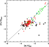 |
Fig. 1. Metallicities derived from SDSS spectra (LR) compared to those of independent analysis of the same stars (ext). The black dots are the TOPoS sample (see text); the data are provided in Table B.1. The red dots are the PASTEL sample (see text); the data is provided in Table B.2. The green dots are data from Caffau et al. (2018), and open symbols are stars with uncertain abundance according to Caffau et al. (2018). The blue dots are data from Caffau et al. (2020). The stars circled in black are removed from the average (see text). |
We hence adopted 0.35 dex as the accuracy of our spectroscopic metallicities. This is probably an upper limit to the actual accuracy, because it does not take into account the errors of the external metallicities. There is also an indication that our metallicity estimates are 0.1−0.2 dex too high.
4. Cross-match with Gaia and down selection
As soon as the metallicities from our processing of the SDSS spectra became available, we began to look at the MDF resulting from this sample. It was obvious that there was a clear excess of metal-poor stars, which we suspect is due to the presence of cool white dwarfs, some of which show Ca II K absorption, as suggested by visual inspection of a few spectra. We therefore cross-matched our catalogue with Gaia to use parallaxes to remove white dwarfs from the sample. To construct the Gaia colour-magnitude diagram, we need to correct the colours for the effect of reddening. To be on the same scale as SDSS, we used the extinction in the g band, Ag, provided in the SDSS catalogue. The reddening on the Gaia colours was estimated in three steps: AV = Ag/1.161; E(B − V) = AV/3.1; correct E(B − V) as in Bonifacio et al. (2000), AVC = 3.1 × E(B − V)C; (GBP − GRP)0 = 1.289445 E(B − V)C; G0 = G − 0.85926 AVC. The extinction coefficients are adopted from the PARSEC website4 (Bressan et al. 2012) and correspond to a G2V star, assuming the extinction laws by Cardelli et al. (1989) plus O’Donnell (1994), and a total-to-selective extinction ratio of 3.1. The cross-match with Gaia left us 290 498 spectra for 245 838 unique stars. For a large part of the sample, the parallaxes were very poor, leading to implausibly high luminosities for such stars.
The Gaia photometry, with a typical intrinsic precision of a few mmag, gives us the opportunity to clean the sample of stars with inaccurate SDSS photometry. We started from the (g − z)0 versus (GBP − GRP)0 plane, shown in Fig. 2. We fitted a straight line5 and selected only the stars for which the observed (GBP − GRP)0 was within ±3σ of the fitted value. We assume that the stars that fall out of this strip have either systematic errors in their g − z colours or are highly reddened. Either way, the Teff used in the MyGIsFOS analysis is wrong; therefore, we discarded these stars. To exclude all the very-low-luminosity stars, which we assume to be mostly cool white dwarfs, we also cut on absolute magnitude, excluding stars with G0, abs > 7.0. Since many of the stars in our sample have poor parallaxes, we decided to use the distance estimates of Bailer-Jones et al. (2018) to perform this cut.
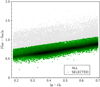 |
Fig. 2. (g − z)0 versus (GBP − GRP)0. The full dataset is shown as grey dots; the green dots are the selected stars. |
These geometric distances are the result of a Bayesian estimate, based on the prior of an exponentially decreasing space density. The exponential length scale varies as a function of Galactic coordinates (l, b). For each star, an estimated distance is provided, rest, as well as a ‘highest distance’ rhi and ‘lowest distance’ rlo. Over the whole catalogue (1.33 × 10⁹ stars), the 50th percentile of the difference rhi − rlo is about 3.6 kpc. This selection results in 171 645 spectra for which MyGIsFOS has converged. This resulted in 139 943 unique stars.
The colour-magnitude diagram (CMD) of the selection is shown in Fig. 3. The cleaned sample thus appears to be compatible with a sample of old TO stars, as is our intention. In Fig. 4, we show the histogram of the semi-dispersion of the geometric distance estimates from Bailer-Jones et al. (2018).
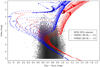 |
Fig. 3. CMD with the selection using Gaia photometry and parallaxes. Two sets of Parsec isochrones (Bressan et al. 2012) of ages 1−14 Gyr and metallicities −0.5 (red) and −1.5 (blue) are shown. The absolute magnitudes were computed assuming the distances of Bailer-Jones et al. (2018). |
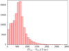 |
Fig. 4. Histogram of the distance errors in pc, from the geometric distances of Bailer-Jones et al. (2018), estimated as 0.5 × (Dmax − Dmin). |
5. Bias in the observed spectroscopic metallicity distribution function
Our sample consists of 139 493 unique stars for which we derived metallicities from at least one SDSS spectrum. For stars with multiple spectra, each spectrum was independently analysed, and then the derived metallicities were averaged (see Sect. 3.1). Our spectroscopic sample contains stars that have been observed in four different SDSS programs, comprising 39 different surveys. It seems arduous to extract the bias in our sample starting from the selection criteria of the different surveys convoluted with our own selection criteria. In Table 1, we assembled the programmes and the types of our sample of spectra, with the numbers for each. We note that 6425 spectra have a blank type, for 6221 targets the type is ‘not available’ (NA), and for 20 973 it is STAR. The largest fraction of our targets are NONLEGACY. We were unable to find any reference to this type of target in the SDSS documentation, and so we may guess that these are essentially ‘fill fibres’ to complete a plate, with no particular selection criterion. The sample is in fact dominated by these targets and spectro-photometric standards. We therefore employed a different route to estimate the bias in our sample.
Target types and SDSS programs for which the spectra have been observed.
5.1. Photometric metallicities
We began by determining metallicities using a photometric index that is metallicity sensitive. The obvious choice would be u − g; however, we preferred to use a reddening-free index that can be formed combining u − g and g − z:

The choice of the colours to form the p index is dictated by the need to have a metallicity-sensitive colour, the fact that u − g is the most metallicity-sensitive colour in ugriz photometry, and the need to factor out the temperature sensitivity of the same index. The choice of g − z has been done to be consistent with the colour chosen to determine effective temperatures. The coefficient in front of g − z is nothing other than the ratio of the two reddening coefficients as provided by Schlegel et al. (1998) in order to make p reddening free. In fact, p is nothing other than the ugz equivalent of the Q index introduced by Johnson & Morgan (1953) for UBV photometry.
The p index varies with effective temperature, surface gravity, and metallicity, as illustrated in Fig. 5, where we show the spectroscopic metallicities on the x-axis. It is clear that a spread in p at any given metallicity remains, even by fixing the effective temperature of the sample. This is because p is also sensitive to log g, and the set of a few stars that are around metallicity −1.5 and p ≈ 0.9 also contains horizontal-branch stars. In order to obtain a metallicity, we adopted a very simple approach: we derived Teff from the (g − z)0 colour, and once the Teff is known, we derived the surface gravity using the parallax and the Stefan-Boltzmann equation, assuming a mass of 0.8 M⊙. Once Teff and log g were known, we only needed to interpolate in a grid of theoretical values to obtain a metallicity from the observed p index.
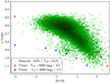 |
Fig. 5. p index as a function of metallicity for stars with 5875 K ≤ Teff ≤ 6125 K compared with theoretical predictions for log g = 4.0 (red) and log g = 2.0 (blue), derived from the Castelli & Kurucz (2003) grid of ATLAS 9 model atmospheres. For the observed stars, we show the spectroscopic metallicities. |
We computed the theoretical p index for the Castelli & Kurucz (2003) grid of ATLAS 9 model atmospheres. The procedure needs to be iterated, since to determine the surface gravity one needs to know the bolometric magnitude. The latter can be derived from the GaiaG0 magnitude and a theoretical bolometric correction that we computed for all the Castelli & Kurucz (2003) grid. To do this, one needs to know the metallicity. In this sense, the procedure is iterative: one starts from a guess of the metallicity to determine the bolometric correction and then computes the metallicity. At that point, with the new metallicity, one derives a new bolometric correction and iterates the procedure. In the vast majority of cases, a single iteration was sufficient. Bolometric corrections for the G magnitude are small for TO stars anyway. In order to accelerate the procedure, we did not interpolate in the grid of theoretical p values for the current Teff and log g, but we simply used the grid values that are nearest. In order to be able to use the method, we need parallaxes for all the stars. For the majority of the stars in our spectroscopic and photometric samples, the Gaia parallaxes are too uncertain to be used. Therefore, to derive the metallicities we used the distance estimates provided by Bailer-Jones et al. (2018), which were derived from Gaia parallaxes using a Bayesian estimate and a prior of exponentially decreasing stellar density. The procedure to determine the metallicities from the p index is explained in detail in Appendix C.
In Fig. 6, we show the comparison of photometric and spectroscopic metallicities. Aside from the large scatter, which we attribute mainly to the large uncertainty in the photometric metallicity estimate, the two variables are tightly correlated. We interactively selected a sub-set of 118 158 stars that lie along the highest density ridge and fitted a straight line (shown in blue) to derive the spectroscopic metallicity from the photometric metallicity.
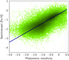 |
Fig. 6. Spectroscopic metallicity as a function of the metallicity derived from the p index. The blue line is a linear fit we made to the sub-set of stars along the highest density ridge. |
By construction, these ‘adjusted’ photometric metallicities (i.e. not those derived directly from p using the procedure in Appendix C, but those derived from the latter and the straight line fit shown in Fig. 6) have a distribution that is similar to that of the spectroscopic metallicities.
5.2. Comparison with a larger photometric sample
In order to estimate the bias in our spectroscopic sample, we make the bold assumption that a sample selected from the SDSS DR12 photometry, using the same colour and absolute magnitude cuts that have defined our spectroscopic sample, is bias-free. Having selected the sample, we applied to it our photometric calibration. The distances were adopted from the Bailer-Jones et al. (2018) catalogue, and we discarded about one million stars whose colours fall outside our synthetic grid. The final sample, which we refer to in the following as ‘photometric’, consists of 24 037 008 unique stars.
In Fig. 7, we show the two samples in the diagram of height above the Galactic plane and distance from the Galactic centre. We adopted a distance of 8.43 kpc for the Galactic centre (Reid et al. 2014) and a distance of the Sun above the Galactic plane of 27 pc (Chen et al. 2001). The photometric sample reaches higher values of |z| and larger distances from the Sun. This is a result of the fact that the photometric sample has many more faint stars than the spectroscopic sample. We computed the bias using the full sample (see Sect. 5.3) and also using a sub-set of the photometric sample that covers the range in |z| and RGC occupied by the spectroscopic sample more closely. The difference in the derived bias is negligible.
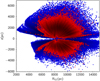 |
Fig. 7. Spectroscopic (red) and photometric (blue) samples in distance from the Galactic centre and height above the Galactic plane. |
We can now compare the two metallicity distributions. In Fig. 8, the distributions of the photometric metallicities of the two samples are compared. It is clear that the spectroscopic sample is boosted in metal-poor stars. An obvious reason for this is the large number of spectrophotometric standards that are part of the sample. These stars are selected to have colours consistent with metal-poor F dwarfs to allow a reliable flux calibration of the spectra on the same plate. We suspect that many of the NONLEGACY targets were selected according to similar criteria. These two contributions alone could explain the boost of metal-poor stars in the spectroscopic sample.
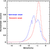 |
Fig. 8. Distribution of photometric metallicities for the photometric and spectroscopic samples. Each sample has been normalised so that the area under the histogram is equal to one. |
5.3. Correcting for the bias
A straightforward way to correct our sample for the selection bias is to take the ratio of the two histograms in Fig. 8, (photometric sample)/(spectroscopic sample), to derive a ‘bias function’. This function is shown in Fig. 9 and relies on photometric metallicities in both samples. In the same plot, we also show a smoothed version of the bias function (median filter with a 0.25 dex kernel) that avoids the oscillations seen at the extremes of the metallicity range that are due to the small number of stars contained in each bin in either of the two histogram functions. We can then produce a bias-corrected version of the histogram of our spectroscopic metallicities, simply by multiplying the observed histogram with this bias function. This rests on the assumption that the bias in spectroscopic metallicities is the same as that in photometric metallicities. Or to put it another way, if we had an SDSS spectrum for each of the stars in the photometric sample and derived a spectroscopic metallicity for it, the bias derived dividing the histogram of these spectroscopic metallicities by that of the spectroscopic metallicities of the current spectroscopic sample would be the same as that shown in Fig. 9.
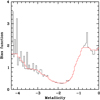 |
Fig. 9. Bias function (black line) and smoothed bias function (red line). |
The result of this exercise is shown in Fig. 10, where the observed and bias-corrected MDFs are shown for our spectroscopic sample. Two features in the bias-corrected MDF are obvious: (i) the bi-modality disappears and the metal-poor peak is now detectable only as a change in the slope of the MDF; and (ii) the slope of the MDF from a metallicity ∼ − 1.6 is much more gentle than in the observed MDF.
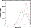 |
Fig. 10. Raw metallicity distribution function (black line) and bias-corrected (red line). |
6. The MDF
Previous investigations of the MDF used different techniques. To keep the comparison to our results manageable, we selected just three MDFs: Schörck et al. (2009, Hamburg/ESO Survey, hereafter HES), Naidu et al. (2020, H3 Survey), and Youakim et al. (2020, Pristine Survey). The first two are based on spectra, while the third uses a photometric metallicity estimate. Our MDF is provided in Table 2.
Raw and corrected metallicity distribution functions for the 139 493 unique stars of our sample.
The HES MDF is derived from a sample of metal-weak candidates selected from the objective prism spectra (see Christlieb et al. 2008), then observed at low resolution (R ∼ 2000) with several telescopes and spectrographs, to provide a sample of 1638 unique stars.
The H3 sample presented in Naidu et al. (2020) is selected with the following conditions: (i) 15 < r < 18; ϖ − 2 × σϖ < 0.5; |b| > 40°. Naidu et al. (2020) claim that this sample is unbiased with respect to metallicity.
The stars selected by H3 are observed with the multi-fibre Hectoechelle spectrograph (Szentgyorgyi et al. 2011) on the 6 m MMT telescope (Conroy et al. 2019). The spectra cover the range 513−530 nm at a resolving power R ∼ 23 000. Using the MINESweeper code (Cargile et al. 2020), an analysis of the spectra combined with photometry provides radial velocities, spectrophotometric distances, and abundances ([Fe/H] and [α/Fe]).
The Pristine sample is aimed at selecting the tip of the main-sequence turn-off of the old populations of the Galaxy using SDSS photometry. A magnitude cut was applied to select stars with 19 < g0 < 20 and colour 0.15 < (g − i) < 0.4, combined with the exclusion of a region in the (u − g)0 versus (g − i)0 plane that is dominated by young stars (see Fig. 3 of Youakim et al. 2020). This sample amounts to about 80 000 stars. A bias correction of the sample is proposed to correct for the selection effects and for the photometric errors.
We did not compare to the MDF of Allende Prieto et al. (2014), because its metal-weak tail is essentially identical to ours, as is expected, since there is a substantial overlap between the two sets of spectra, although the spectra were analysed in different way. No bias correction was attempted in Allende Prieto et al. (2014). With respect to our sample, the Allende Prieto et al. (2014) sample lacks the metal-rich peak, and this is just a matter of selection criteria.
6.1. Comparison with H3
We carried out a more detailed comparison with H3, since it is the one that is more easily directly comparable to our results. Both are based on spectroscopy, and an MDF is available up to super-solar metallicities.
Here, and in Sect. 8, we need to define sub-samples that make use of parallaxes. For this reason, we need to define a sub-set with ‘good’ parallaxes. We define this sample as stars for which ϖ > 3 × Δϖ, which leaves us with a sample of 57 386 unique stars. In terms of metallicity distribution, this sub-sample favours the metal-rich component, so that now the most prominent peak is the metal-rich one, as shown in Fig. 11. On the other hand, the metal-weak tail of the two distributions is pretty much the same. In the following, we refer to this sub-sample as the good parallax sample. To have more meaningful comparison between the H3 MDF and our sample, we selected a sub-sample of our good parallax sample, which fulfils the same selection criteria as Naidu et al. (2020). This is composed of 28 165 stars, which is 49% of our good parallax sample. We refer to this sub-sample as the H3-like sample. In Fig. 12, we compare the normalised MDFs of our good parallax and of our H3-like samples to that of Naidu et al. (2020).
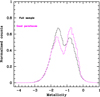 |
Fig. 11. Normalised metallicity distribution of our full spectroscopic sample (black) compared to the subset with good parallaxes (violet). The normalisation is such that the area under each histogram is equal to one. |
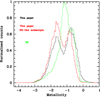 |
Fig. 12. Normalised MDFs for our sample with good parallaxes (black line), the sub-sample selected according to the criteria of H3 (red line) and the H3 (Naidu et al. 2020, green). |
From this comparison four facts are obvious: our sample is boosted in metal-poor stars with respect to an unbiased sample, confirming what was deduced from the comparison with our photometric sample. A H3-like selection, although it does not make any explicit reference to metallicity, is likely to introduce a bias in metallicity. This can be inferred by the comparison of our good parallax and H3-like samples. It is, however, obvious that this bias is minor, especially in the low-metallicity tail, and we ignore it in the following. The H3 MDF has a much more gentle slope of the metal-weak tail than our sample. The metal-rich peak in our full sample seems very similar to that in the H3 sample.
6.2. The metal-weak tail of the MDF
While the metal-rich portion of the MDF is the result of the complex chemical evolution of the Galaxy, we may assume that its metal-weak tail is much simpler, since many of the stars are the descendants of only a few generations of stars beyond the first one. For more than a decade, theoretical models have shown that the properties of the first stars affect the metal-weak tail of the MDF (e.g. Hernandez & Ferrara 2001; Prantzos 2003; Oey 2003; Karlsson 2006; Tumlinson 2006; Salvadori et al. 2007). Furthermore, this should hold true even if this metal-weak tail contains stars that have been formed in Milky Way satellites that later merged to form the present-day Milky Way (e.g. Salvadori et al. 2015).
To study the metal-weak tail of the MDF, Schörck et al. (2009) normalised their distributions at metallicity −1.95. This normalised distribution provides, for any lower metallicity, the fraction of stars in that metallicity bin, with respect to those in the bin centred at −1.95. We use the same approach, which also allows us to directly compare our results with theirs.
In Fig. 13, we compare the normalised metal-weak tail of the MDF, as observed, for (i) our whole sample; (ii) the Hamburg/ESO sample (Schörck et al. 2009; iii) the Pristine sample (Youakim et al. 2020); and (iv) the H3 sample (Naidu et al. 2020). The H3 Survey adopts a target selection that is based only on apparent magnitudes, parallaxes, and Galactic latitude, thus they claim that their sample is unbiased with respect to metallicity. It is surprising that the metal-weak tail of their MDF is essentially identical to that of the Hamburg-ESO Survey down to metallicity −3.0, since the Hamburg/ESO Survey has been considered to be biased in favour of metal-poor stars (Schörck et al. 2009). The abrupt drop of the H3 MDF at −3.0 is not easy to understand, but it may be due to the fact that the size of their sample is too small to adequately sample the populations of lower metallicity.
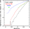 |
Fig. 13. Metal-weak tail of the raw metallicity distribution function (black line), normalised at −1.95, compared with the MDFs of the Hamburg/ESO survey (Schörck et al. 2009, red), the Pristine survey (Youakim et al. 2020, blue), and the H3 survey (Naidu et al. 2020, green). |
The selection function for the four samples is clearly different. Schörck et al. (2009) provide three possible bias corrections for their observed MDF, while Youakim et al. (2020) provide two. In Fig. 14, we show the comparison with all the corrected MDFs. What is obvious is that while in the raw distributions ours is always below the Hamburg/ESO, once bias corrections are taken into account ours is above the Hamburg-ESO. As noticed in Sect. 5.3, this is due to the fact that in our corrected MDF, the slope is much more gentle than in our raw MDF; as a consequence, once we normalise at −1.95, the corrected MDF lies above the raw MDF. The reverse is true if we look at the non-normalised MDF, as shown in Fig. 10.
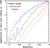 |
Fig. 14. Metal-weak tail of the corrected metallicity distribution function (black line), normalised at [Fe/H] = −1.95, compared with the corrected Hamburg/ESO (Schörck et al. 2009, red) and the corrected Pristine (Youakim et al. 2020, blue) MDFs. |
Above metallicity −3.0 the H3, the uncorrected HES, and our corrected MDF are essentially identical. If we make the assumption that our bias-corrected MDF is ground truth, then the metallicity bias of the H3 and HES MDFs must be small, and in fact negligible. We thus conclude that it is legitimate to use the average of these three MDFs for comparison with theoretical models. The assumption we are making is equivalent to stating that the bias corrections provided by Schörck et al. (2009) and Youakim et al. (2020) are not adequate to describe the actual bias in their stellar sample. The bias corrections proposed by Schörck et al. (2009) are based on models, while those of Youakim et al. (2020) are based on the statistical properties of the sample. One advantage of using the average is that in each metallicity bin the standard deviation can be used as an error estimate on the MDF. A further advantage is that the averaging process makes the statistical errors smaller. The H3 MDF is essentially undefined below −3.0; therefore, we suggest only using the average of our MDF and that of HES in this metallicity range. In Fig. 15, we show the two average values with the standard deviation in each bin. The values are provided in Table 3.
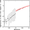 |
Fig. 15. Average metal-weak tail of the MDF, normalised at metallicity −1.95: black present paper (corrected) and Hamburg/ESO (uncorrected) red; the H3 is also included in the average. |
Average MDF, normalised at metallicity −1.95.
7. 3D bias and metallicity maps
We can now take advantage of the precise measurements of metallicity and position for our large stellar sample to study the spatial distribution of stars with different metallicities as has been suggested by cosmological models (e.g. Salvadori et al. 2010). To achieve this goal, we need to derive the 3D bias function, meaning that we also need to study how the bias function depends on the position of the stars. To this aim, we adopt the cylindrical coordinates |z| and  and divide the space in annuli of radial width dR = 0.5 kpc and height dz = 0.3 kpc. In each annulus, the photometric MDFs from the spectroscopic and photometric samples have been derived and used to compute the local bias function by adopting metallicity bins of 0.25 dex. In the following, we use Fe to denote the metallicity, as defined in Sect. 2. From a global point of view, this means that we have constructed a 3D bias function, Bias = Bias(Fe, ρ, |z|), that we can use to compute the correct local MDF and to construct stellar metallicity maps.
In Fig. 16, we show a simplified view of the 3D bias function obtained by dividing the stellar populations into different metallicity ranges: extremely metal-poor stars (−4 ≤ [Fe/H] < −3, upper left panel), very metal-poor stars (−3 ≤ [Fe/H] < −2, upper right), metal-poor stars (−2 ≤ [Fe/H] < −1, lower left), and metal-rich stars (−1 ≤ [Fe/H] < 0, lower right). Colours in the maps illustrate the value of the bias obtained in each annulus, which is identified by a single pixel in the (ρ, |z|) space. A bias equal to zero means that there are no stars from the spectroscopic sample within the pixel, which is indeed the case for extremely metal-poor stars (upper left) located in the outermost regions (|z| > 3 kpc, ρ > 10 kpc).
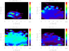 |
Fig. 16. Bias maps in the cylindrical coordinate plane (ρ,|z|). Each panel shows the results for different stellar populations (see labels). |
Bearing in mind that the colour-bar scale is different in each panel, we can notice several features in Fig. 16. First, the contrast between the minimum and maximum values of the bias is higher for very and extremely metal-poor stars ([Fe/H] < −2, upper panels), where it reaches values of Bias > 5 in several small and isolated regions. Our analysis shows that these extreme bias values are a result of the small statistic in the considered pixel. Conversely, the bias is much more uniform for metal-poor stars (lower left panel), only spanning an interval of two in spite of the more extended regions covered by the map. The contrast between minimum and maximum bias increases again for metal-rich stars, as seen in the lower right panel of Fig. 16, where we can notice three zones with Bias ≥ 2. The high contrast between the bias in these isolate small regions, and the rest of the space is at the origin of the oscillations seen in the (1D) bias function analysed in Sect. 5.3 (Fig. 9).
A more intuitive view of the bias function showing its dependency on the single variables ρ and |z| is presented in Fig. 17 (upper panels), while we refer the reader to Fig. 9 (Sect. 5.3) for the metallicity dependence. The 1D bias functions shown in Fig. 17 were obtained starting from the spectroscopic and photometric samples from which we derived the radial and height stellar distributions displayed in the same figure (lower panels). The upper left panel of Fig. 17 shows how the bias function varies with the radius ρ. We notice that Bias(ρ) is maximum at the lowest radii, and it rapidly declines towards larger ρ, reaching its minimum at ρ ≈ 8.5 kpc, and then it rises again. This behaviour can be easily understood: the position of the minimum corresponds to the position of the Sun, ρ = 8.43 kpc (see Sect. 5.2), and hence it identifies the radius where the number of stars in the spectroscopic sample is larger, N * ≈104, as can be seen in the lower left panel of Fig. 17. In the same panel, we see that both at smaller and larger radii the number of stars in the spectroscopic sample decreases, reaching the value N * ≤400 at the extremes. Conversely, the number of stars in the photometric sample remains roughly at the constant value of N * > 106 for 6.5 kpc < ρ ≤ 10 kpc and slowly declines at larger ρ, following the same trend of the spectroscopic sample. This behaviour drives the shape of the bias function, which we remind the reader is obtained by dividing the photometric and the spectroscopic metallicity distributions (see Sect. 5.2 for more details).
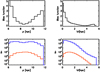 |
Fig. 17. Variation of the bias function with the cylindrical radius, ρ (left upper panel), and the height above the Galactic plane, |z| (right upper panel). Lower panels: distribution of stars from the photometric (blue) and spectroscopic (red) samples as functions of ρ (left) and |z| (right). |
The variation of the bias function with |z| is shown in the right upper panel of Fig. 17. We see that Bias(|z|) is maximum on the Galactic plane and then it rapidly decreases at higher |z|, reaching values close to zero for |z| ≈ 4 kpc. We can also notice a little bump at |z| ≈ 5 kpc. Once again, these trends can be understood by looking at the effective number of stars from the spectroscopic and photometric samples in each |z| bin (lower right panel of Fig. 17). We see that the number of stars in the spectroscopic sample gradually increases with |z|, reaching the maximum N * ≈104, at |z| ≈ 1 kpc, and then rapidly declining at higher z. Conversely, the number of stars in the photometric sample is maximum close to the Galactic plane, |z| ≤ 0.5 kpc, and then it starts to decline. This explains the trend of the bias function with |z|.
We note that at |z| > 4 kpc the spectroscopic sample is very poorly represented, N * < 100, which means that the bump observed in Bias(z) at |z| ≈ 5 kpc is driven by a very small number of stars, N * < 10. To understand the origin of this bump we should inspect the complete 3D bias maps shown in Fig. 16 again. With the exception of metal-poor stars (left lower panel), all stellar populations show zero bias at |z| ≥ 4 kpc for all ρ. This means that there are no stars in the spectroscopic sample in these regions and at these metallicities. At |z| ≈ 5 kpc (ρ ≈ 7.5 kpc) instead, very metal-poor stars show a small isolated ‘island’ with Bias ≈ 1.5. It is likely this small region, counting < 10 stars, which originates the small bump, observed Bias(z) at |z| = 5 (right upper panel).
In Fig. 18, we show the spatial distribution of extremely metal-poor, very metal-poor, metal-poor, and metal-rich stars corrected for the bias. In other words, these maps were obtained by multiplying the raw spatial distributions of the spectroscopic sample for the local 3D bias function. In Fig. 18, we can first notice that the spatial distribution of extremely metal-poor stars (EMPs, left upper panel) is completely different with respect to those of the more metal-rich stellar populations (i.e. [Fe/H] > −3). EMPs are clustered in a smaller region of the (ρ, |z|) plane, and their spatial distribution does not appear uniform like the others do. This is most likely a consequence of the low number of statistics: in the three main regions filled by EMPs, we can indeed see that the number of stars per pixel is < 15. Conversely, more metal-rich stars cover almost the same regions of the (ρ, |z|), and they are all much better represented in each pixel, where N * > 30 most of the time. However, we can notice that the maxima of the stellar distributions (red regions) reside in three different locations, which implies that there are spatial gradients in the metallicity distribution function. A more in-depth and quantitative analysis of these results, which includes a comparison with cosmological models, is beyond the scope of the present paper and will be presented in our future work (Salvadori et al., in prep.).
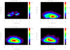 |
Fig. 18. Distribution of extremely metal-poor (upper left), very meta-poor (upper right), metal-poor (lower left), and metal-rich (lower right) stars in the cylindrical coordinate plane (ρ,|z|). The distributions have been corrected using the 3D bias function. |
8. Dynamical properties of the SDSS spectroscopic sample
In order to discuss the dynamical properties of the sample, we only make use of the good parallax sample. In terms of Galactic location, the two samples occupy approximately the same space in the RGC, z plane, as shown in Fig. 7. We corrected the Gaia parallaxes for the global zero point of −0.029 mas (Lindegren et al. 2018). With these parallaxes, the Gaia proper motions, and the SDSS radial velocities, we used the galpy code6 (Bovy 2015) to evaluate orbital parameters and actions under the Staeckel approximation (Binney 2012; Mackereth & Bovy 2018) and using the MWPotential2014 potential (Bovy 2015).
8.1. The Gaia-Sausage-Enceladus structure
From the studies of Belokurov et al. (2018), Haywood et al. (2018), Helmi et al. (2018) and Di Matteo et al. (2019), we know that the Galactic halo7 is dominated by stars that were accreted from a galaxy that we refer to as Gaia-Sausage-Enceladus (GSE). The precise dynamical definition of this object is still not known. We refrain from identifying, in dynamical spaces, multiple accretion events (Naidu et al. 2020) and small sub-structures, since we are aware that, from the theoretical point of view, a single massive accretion event can give rise to several dynamical sub-structures (Jean-Baptiste et al. 2017). We therefore concentrate on isolating GSE, although we are aware that it is practically impossible to identify a ‘pure’ sample of GSE stars, since one of the outcomes of the accretion is that stars that come from both the accreted satellite galaxy and the accreting galaxy will end up in the same region of any dynamical space. Chemical information may be helpful to disentangle the accreted from the accreting, but our information is limited to an average metallicity and is not sufficient for this purpose.
Based on dynamical data and photometric metallicities, Feuillet et al. (2020) suggested that the best way to select a pure GSE sample is in the space of angular momentum Lz and radial action (Jr, or its square root). In Fig. 19, we show such a diagram for our good parallax sample. The points in blue correspond to the GSE selection of Feuillet et al. (2020), namely −500 kpc km s−1 < Lz < 500 kpc km s−1 and 30 (kpc km s−1)1/2 <  (kpc km s−1)1/2.
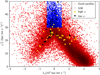 |
Fig. 19. Diagram of angular momenta and square root of the radial action. Our good parallax sample is shown via red dots, the blue rectangle is the GSE selection proposed by Feuillet et al. (2020), the yellow dots are the high-α stars of Nissen & Schuster (2010), while the black dots are their low-α stars. |
The existence of two sequences of [α/Fe] in the solar neighbourhood as a function of metallicity was initially discovered by Fuhrmann (1998, and subsequent papers) and later confirmed by Nissen & Schuster (2010), who introduced the terms low-α and high-α stars. Haywood et al. (2018) demonstrated convincingly that the low-α stars should be associated with GSE, while high-α are stars formed in the Milky Way. This was also later confirmed by Helmi et al. (2018). In Fig. 19, we also plot the stars classified as low α and high α by Nissen & Schuster (2010). Seventeen of the Nissen & Schuster (2010) stars fall in the Feuillet et al. (2020) GSE selection box; of these, fourteen are low-α stars and three are high-α stars. This allows us to estimate that the Feuillet et al. (2020) GSE selection box includes about 18% of stars that are not associated with GSE. This confirms the theoretical expectation that it is impossible to dynamically select a pure sample of the accreted stars. In the case of the Nissen & Schuster (2010) stars, the chemical information allows one to disentangle the two populations; however, the two α/Fe sequences merge at metallicities lower than about −1.0, making this chemical diagnostic unusable. Pragmatically, we decided to adopt the Feuillet et al. (2020) selection, keeping in mind that there will be a contamination, since this appears to be the least contaminated selection of GSE. We would also like to point out that there is also no guarantee that this selection of GSE provides an unbiased sample of the stars of the accreted galaxy.
The Feuillet et al. (2020) selection contains 3227 stars in our good parallax sample. Since this sample was extracted from a biased sample of stars, this MDF cannot be taken as representative of the MDF of GSE. On the other hand, we cannot apply the bias correction that has been derived for the global sample, since this sub-sample has, a priori, a different bias. We cannot apply the Feuillet et al. (2020) selection to the photometric sample to derive an appropriate bias function, since we lack the radial velocities necessary to derive Lz and Jr. However, in Sect. 7 we derive the space dependence of the bias function. We can therefore divide the GSE sample into bins in the ρ, |z| space and apply the appropriate bias function to each bin.
The bias correction results in shifting the MDF to higher metallicities, as expected; however, our MDF remains distinctly more metal-poor than that derived by Feuillet et al. (2020), as shown in Fig. 20. Both our raw and bias-corrected MDF of GSE lack the significant population between −1.0 and solar metallicity that is present in the Feuillet et al. (2020) MDF of GSE. Our MDF is also slightly narrower than that of Feuillet et al. (2020). Although the shape of none of the MDFs is Gaussian, a Gaussian fit can provide a measure of their width. Our MDFs (both raw and bias-corrected) have a full width at half maximum of about 0.6 dex, while that of Feuillet et al. (2020) is about 0.7 dex.
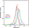 |
Fig. 20. Observed metallicity histogram of GSE, for the whole sample (black), and the bias-corrected histogram (red). The histogram of Feuillet et al. (2020) is shown in blue, while that of Naidu et al. (2020) is shown in green. |
A possible reason for the discrepancy is that the Casagrande et al. (2019) photometric calibration, which is used by Feuillet et al. (2020) to derive the metallicities, is validated only down to −2.0. Thus, the Feuillet et al. (2020) sample may have been selected with a bias against metal-poor stars. To gain some insight into a comparison of our metallicities and those obtained from the Casagrande et al. (2019) calibration, we cross-matched our sample with Skymapper DR 1.1 (Wolf et al. 2018) and with 2MASS (Skrutskie et al. 2006). We found a sub-sample of 20 203 unique stars, and we applied the Casagrande et al. (2019, Eq. (12)) calibration. This photometric metallicity correlates only weakly with our spectroscopy metallicity. The metallicity distributions of the same stars using the two different metallicity indicators do not resemble each other. The photometric metallicity is on average 0.7 dex more metal rich, but with a dispersion that is of the same order of magnitude. We do not want to push this comparison further, since our stars are dwarfs, while those used by Feuillet et al. (2020) are giants, and the systematics may well be different.
Naidu et al. (2020) also provide an MDF for GSE, and this is shown in Fig. 20. Their MDF is similar to that of Feuillet et al. (2020) around the peak, but it departs from it both in the metal-weak and in the metal-rich tail. It is clearly different from ours, that has many more metal-poor stars. We point out that the Naidu et al. (2020) selection of GSE is very different from that of Feuillet et al. (2020) and adopted by us. In fact, they write the following: “We select GSE stars by excluding previously defined structures and requiring e > 0.7”. Hence, it is necessary to have previously isolated all the different sub-structures identified by Naidu et al. (2020). In order to mimic the Naidu et al. (2020) selection, we selected stars with e > 0.7 and −500 kpc km s−1 < Lz < 500 kpc km s−1 in our sample. This translates, in our preferred selection plane, to 18 (kpc km s−1)1/2 <  (kpc km s−1)1/2. As stated above, this increases the contamination of stars not related to GSE, probably above the level of 50%, as estimated from applying this selection to the Nissen & Schuster (2010) sample. It is, however, not clear if these contaminating stars have an MDF different from GSE or not. We applied this selection to our sample, and the MDF we obtain is similar to what we obtain with the Feuillet et al. (2020) selection. As in the case of Feuillet et al. (2020), we may suspect that the metallicity scale of Naidu et al. (2020) is different from ours. This seems unlikely since the metal-weak tail of our bias-corrected MDF agrees very well with that of Naidu et al. (2020). A more detailed comparison will have to wait until the H3 catalogue is fully published and metallicities of known stars can be compared.
We can, however, comment on the similarity of the peak position between Feuillet et al. (2020) and Naidu et al. (2020), in spite of their disagreement in both metal-weak and metal-rich tails. Both Feuillet et al. (2020) and Naidu et al. (2020) rely on giant stars. However, neither takes into account the fact that the rate at which the stars leave the main sequence is metallicity dependent (the evolutionary flux; see Renzini & Buzzoni 1986) or the fact that the rate of evolution along the red giant branch is also metallicity dependent (Rood 1972). These effects were discussed in the case of the Galactic bulge by Zoccali et al. (2003). It may well be that the similarity in the peak of the MDFs of GSE of the two above-mentioned studies does in fact signal that both these MDFs are biased by the choice of tracers, namely giant stars8.
It is remarkable that the slope of the metal-weak tail of the MDF of GSE is much steeper than what was obtained from the full sample, as shown in Fig. 21. This is true even if we consider our observed MDF, before bias correction; thus, it must be considered as a very robust finding. It could be argued that rather than comparing the GSE MDF to our mean MDF, which also relies on our 1D-corrected MDF, we should have used our 3D-corrected MDF for the full sample. There are two reasons for not doing this. First of all, in the metallicity range that is relevant for GSE, the 1D-corrected and 3D-corrected MDFs are pretty close, while they become increasingly different at lower metallicities where the 3D bias is plagued by a low number of stars per bin. Secondly, the average MDF has a much smaller error than our 1D-corrected MDF and, a fortiori, than our 3D-corrected MDF.
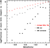 |
Fig. 21. Observed metallicity histogram of GSE, normalised to −1.95 compared to that of the global sample. The global sample is bias corrected as described in Sect. 5.3. The GSE sample is shown both raw and corrected, as described in Sect. 7. |
8.2. Errors on dynamical quantities and consequences on selections
In order to evaluate the uncertainty in the derived kinematical parameters, we used the pyia code9 to generate samples of the six parameters (coordinates, parallax, proper motions, and radial velocity) in input to galpy for each object. Samples are generated from a multi-variate Gaussian distribution, where the errors on the parallax, proper motions, and radial velocity; and the correlation coefficients between parallax and proper motions are only taken into account in the construction of the covariance matrix. One thousand realisations were extracted for each object. The samples were then fed into galpy, and the errors were evaluated as the standard deviations of the obtained orbital parameters, after unbound orbits were rejected. For the error estimate, we only accepted objects for which more than 950 out of 1000 realisations provided meaningful results, namely 54 215 stars over 57 386. When we consider the GSE sub-sample, the number of stars retained drops from 3227 to 2487. We consider that stars that have too few meaningful realisations to have uncertain orbital parameters.
The question is, what is the effect of these errors on a sub-sample selected on the basis of dynamical quantities? We compared the metallicity histograms for the full GSE sample with errors (2487 stars) and for a sub-sample selected with the supplementary condition eLz < 263.983 kpc km s−1 and eJr < 995.473 kpc km s−1, where eLz and eJr are the errors on Lz and Jr derived as described above, and the condition is fixed to the median of the error distribution. From this comparison, it is clear that the shape of the MDF is by and large the same if we consider the full GSE sample or only the sub-sample that has smaller errors on the orbital parameters. We thus conclude that the shape of the MDF for our GSE selection is robustly determined. In the same way, we find that the conclusions are not different if we consider the full sample of 3227 or the sub-sample of 2487 stars with reliable orbital parameters, according to the above definition.
9. Discussion
Our recommended metal-weak tail of the MDF is provided in Table 3. We deduced that the raw Hamburg/ESO MDF is essentially unbiased from its similarity with our own bias-corrected MDF and the H3 MDF. Why would the HES be unbiased, when Schörck et al. (2009) warned that it is biased in favour of the metal-poor stars and provide bias corrections? Our understanding is that globally the HES is biased; however, the follow-up on metal-poor candidates selected from the objective prism spectra has been unbiased for all stars of metallicity below −2.0. Quite likely, this was because of the low resolution of the prism spectra, which made it difficult to discriminate between a −2.0 and a −3.0 star. For this reason, the HES MDF, normalised at −1.95, is effectively unbiased.
Another question is, why does the Pristine MDF show a larger fraction of metal-poor stars at any metallicity compared to the other three MDFs? This needs to be further investigated using the Pristine data. However, we think this may be due to two factors: Youakim et al. (2020) did not use Gaia-based distance estimates to ‘clean’ their sample from white dwarfs, but relied on colour cuts. Our own experience, discussed in Sect. 4, shows how the sample appeared much more clear, manageable, and consistent with isochrones, once we applied a distance cut. Youakim et al. (2020) combined the Pristine filter with SDSS wide-band photometry to derive their metallicities. In Fig. 2, we show how the SDSS photometry can be discrepant with Gaia photometry. It could be that the excess in metal-poor stars is partially due to a fraction of stars with poor SDSS photometry.
Another possible issue to be considered is the lower sensitivity to metallicity of any photometric metallicity based on a narrow-band filter centred on Ca II lines, for warm TO stars, with respect to cool giants. This effect is clearly illustrated in Fig. 11 of Bonifacio et al. (2019). Finally, there is a degeneracy between metallicity and surface gravity that is not accounted for in Youakim et al. (2020) and that could cause part of the discrepancy. It would certainly be useful to re-derive the Pristine MDF after cleaning the sample for stars of too-high absolute magnitude and uncertain wide-band photometry.
The MDF we derived for the GSE sub-structure is clearly at odds with that of Feuillet et al. (2020) and Naidu et al. (2020). We already pointed out how there could be an offset in the metallicity scales. We would like to point out that our sample and the Feuillet et al. (2020) sample do not overlap perfectly in the sampled galactocentric volume. The Feuillet et al. (2020) sample preferentially contains stars with |z|< 1 kpc, while our sample is composed mainly of stars with |z| > 1 kpc. Also, the Naidu et al. (2020) sample covers a very different region in the RGC, |Z|, plane. In particular, their sample pushes to 50 kpc, obviously thanks to the use of giant stars as tracers, while we only used TO stars. If there were any gradient of the metallicity of GSE with z or RGC, one would expect the three samples to provide different MDFs.
10. Conclusions
We used our own analysis of SDSS spectra in order to determine the MDF of the metal-poor component of the Milky Way. The metal-weak part of our MDF is in excellent agreement with that determined by Allende Prieto et al. (2014) from an independent analysis of SDSS spectra. This fact, together with the external comparison of a small sub-set of stars analysed at higher resolution and/or S/N gives us confidence in our spectroscopic metallicity, for which we estimate a precision of 0.1 dex and an accuracy of 0.35 dex. We showed that our sample is biased, in the sense that metal-poor stars are over-represented.
Through a comparison with a sample of stars, that we assume to be unbiased with respect to metallicty, for which we determined photometric metallicites, we derived the bias function. This allowed us to provide the unbiased MDF that is given in Table 2. When considering the metal-weak tail of the MDF, normalised at −1.95, we find that our bias-corrected MDF is essentially identical to that of Naidu et al. (2020) and that of Schörck et al. (2009). We therefore advocate that the best estimate is obtained by averaging these three MDFs. This average MDF and its standard deviation is provided in Table 3, and we recommend using this table for comparisons with theoretical predictions.
In the process of estimating the bias in our spectroscopic sample, we introduced a new photometric metallicity estimate based on SDSS u − g and g − z colours and on distance estimates based on Gaia parallaxes. These estimates, along with effective temperatures and surface gravities, for 24 037 008 unique TO stars is available through CDS.
Thanks to the Gaia distances and proper motions, combined with SDSS radial velocities, we computed Galactic orbits and actions for a sub-set of our spectroscopic sample, characterised by good parallaxes. From this sample, we selected likely members of the GSE structure. We were able to derive the metallicity bias of this GSE sample, looking at the position of these stars in the galaxy. In this way, we derived an MDF for GSE, as shown in Figs. 20 and 21. The most notable result is that the fraction of metal-poor stars in GSE is clearly lower than that observed in the Milky Way. This implies a very different formation and evolution history of GSE with respect to the Milky Way. Furthermore, although the ‘progenitor’ of GSE might contain more metal-poor stars (see e.g. Jean-Baptiste et al. 2017) than what we find in the GSE structure, our result seems to suggest that the metal-poor tail of the Galactic halo is not made by massive dwarf galaxies like the progenitor of GSE, but most likely by smaller (ultra-faint) dwarfs. Indeed, according to ΛCDM models, ultra-faint dwarfs are expected to be the basic building blocks of more massive systems and the formation environment of extremely metal-poor stars (see e.g. Salvadori et al. 2015, and references therein).
One should be aware that in the literature ‘metallicity’ may refer to slightly different quantities; often it is [Fe/H], especially in the older papers, but not always. In Sect. 2, we provide the definition of metallicity used in this paper.
Bond (1981) refers to any star with [Fe/H] < −3 as Population III.

We loosely define the Galactic halo as the stars with a total space velocity higher than 180 km s−1 (Di Matteo et al. 2019).
After the acceptance of the paper, C. Conroy brought to our attention the fact that Naidu et al. (2020) accounted for the evolutionary flux via their selection function. However, the MDFs shown in their figures, from which we have taken the values shown in our figures, are all ‘raw’. C. Conroy (priv. comm.) evaluated the metallicity dependence of an MDF based on giants, using the mock Gaia catalogue of Rybizki et al. (2018) and estimates the effect to be of the order of about 0.05 dex, which is far too small to account for the difference between our MDF of GSE and that of Naidu et al. (2020).
Acknowledgments
This paper is dedicated to the late Roger Cayrel who has inspired the TOPoS survey as well as all of our work on metal-poor stars. He passed away on January 11th 2021, and he will be deeply missed. We are grateful to Bertrand Plez who computed all the metal-poor model atmospheres and associated synthetic spectra used in this paper. We acknowledge useful discussions with David Aguado on the contents of this paper. We gratefully acknowledge support from the French National Research Agency (ANR) funded projects “Pristine” (ANR-18-CE31-0017) and “MOD4Gaia” (ANR-15- CE31-0007). A.J.K.H., H.-G.L., and N.C. gratefully acknowledge funding by Deutsche Forschungsgemeinschaft (DFG, German Research Foundation) – Project-ID 138713538 – SFB 881 (“The Milky Way System”), subprojects A03, A04, A05, and A11. S.S. acknowledges support from the ERC Starting Grant NEFERTITI H2020/808240 and the PRIN-MIUR2017, The quest for the first stars, prot. n. 2017T4ARJ5. This work has made use of data from the European Space Agency (ESA) mission Gaia (https://www.cosmos.esa.int/gaia), processed by the Gaia Data Processing and Analysis Consortium (DPAC, https://www.cosmos.esa.int/web/gaia/dpac/consortium). Funding for the DPAC has been provided by national institutions, in particular the institutions participating in the Gaia Multilateral Agreement. Funding for the SDSS and SDSS-II has been provided by the Alfred P. Sloan Foundation, the Participating Institutions, the National Science Foundation, the US Department of Energy, the National Aeronautics and Space Administration, the Japanese Monbukagakusho, the Max Planck Society, and the Higher Education Funding Council for England. The SDSS website is http://www.sdss.org/. The SDSS is managed by the Astrophysical Research Consortium for the Participating Institutions. The Participating Institutions are the American Museum of Natural History, Astrophysical Institute Potsdam, University of Basel, University of Cambridge, Case Western Reserve University, University of Chicago, Drexel University, Fermilab, the Institute for Advanced Study, the Japan Participation Group, Johns Hopkins University, the Joint Institute for Nuclear Astrophysics, the Kavli Institute for Particle Astrophysics and Cosmology, the Korean Scientist Group, the Chinese Academy of Sciences (LAMOST), Los Alamos National Laboratory, the Max-Planck-Institute for Astronomy (MPIA), the Max-Planck-Institute for Astrophysics (MPA), New Mexico State University, Ohio State University, University of Pittsburgh, University of Portsmouth, Princeton University, the United States Naval Observatory, and the University of Washington. Funding for SDSS-III has been provided by the Alfred P. Sloan Foundation, the Participating Institutions, the National Science Foundation, and the US Department of Energy Office of Science. The SDSS-III website is http://www.sdss3.org/. SDSS-III is managed by the Astrophysical Research Consortium for the Participating Institutions of the SDSS-III Collaboration including the University of Arizona, the Brazilian Participation Group, Brookhaven National Laboratory, Carnegie Mellon University, University of Florida, the French Participation Group, the German Participation Group, Harvard University, the Instituto de Astrofisica de Canarias, the Michigan State/Notre Dame/JINA Participation Group, Johns Hopkins University, Lawrence Berkeley National Laboratory, Max Planck Institute for Astrophysics, Max Planck Institute for Extraterrestrial Physics, New Mexico State University, New York University, Ohio State University, Pennsylvania State University, University of Portsmouth, Princeton University, the Spanish Participation Group, University of Tokyo, University of Utah, Vanderbilt University, University of Virginia, University of Washington, and Yale University.
References
- Adelman-McCarthy, J. K., Agüeros, M. A., Allam, S. S., et al. 2008, ApJS, 175, 297 [NASA ADS] [CrossRef] [Google Scholar]
- Ahn, C. P., Alexandroff, R., Allende Prieto, C., et al. 2012, ApJS, 203, 21 [Google Scholar]
- Alam, S., Albareti, F. D., Allende Prieto, C., et al. 2015, ApJS, 219, 12 [NASA ADS] [CrossRef] [Google Scholar]
- Allende Prieto, C., Fernández-Alvar, E., Schlesinger, K. J., et al. 2014, A&A, 568, A7 [NASA ADS] [CrossRef] [EDP Sciences] [Google Scholar]
- Alvarez, R., & Plez, B. 1998, A&A, 330, 1109 [NASA ADS] [Google Scholar]
- Aoki, W., Beers, T. C., Lee, Y. S., et al. 2013, AJ, 145, 13 [NASA ADS] [CrossRef] [Google Scholar]
- Arenou, F., Luri, X., Babusiaux, C., et al. 2018, A&A, 616, A17 [NASA ADS] [CrossRef] [EDP Sciences] [Google Scholar]
- Bailer-Jones, C. A. L., Rybizki, J., Fouesneau, M., et al. 2018, AJ, 156, 58 [NASA ADS] [CrossRef] [Google Scholar]
- Beers, T. C. 1987, Nearly Normal Galaxies. From the Planck Time to the Present (New York: Springer), 41 [CrossRef] [Google Scholar]
- Beers, T. C., Preston, G. W., & Shectman, S. A. 1985, AJ, 90, 2089 [NASA ADS] [CrossRef] [Google Scholar]
- Belokurov, V., Erkal, D., Evans, N. W., et al. 2018, MNRAS, 478, 611 [Google Scholar]
- Bessell, M. S. 1977, PASA, 3, 144 [CrossRef] [Google Scholar]
- Bidelman, W. P., & MacConnell, D. J. 1973, AJ, 78, 687 [NASA ADS] [CrossRef] [Google Scholar]
- Binney, J. 2012, MNRAS, 426, 1324 [Google Scholar]
- Bond, H. E. 1970, ApJS, 22, 117 [NASA ADS] [CrossRef] [Google Scholar]
- Bond, H. E. 1980, ApJS, 44, 517 [NASA ADS] [CrossRef] [Google Scholar]
- Bond, H. E. 1981, ApJ, 248, 606 [NASA ADS] [CrossRef] [Google Scholar]
- Bonifacio, P., Monai, S., & Beers, T. C. 2000, AJ, 120, 2065 [NASA ADS] [CrossRef] [Google Scholar]
- Bonifacio, P., Caffau, E., François, P., et al. 2011, Astron. Nachr., 332, 251 [NASA ADS] [CrossRef] [Google Scholar]
- Bonifacio, P., Sbordone, L., Caffau, E., et al. 2012, A&A, 542, A87 [NASA ADS] [CrossRef] [EDP Sciences] [Google Scholar]
- Bonifacio, P., Caffau, E., Spite, M., et al. 2015, A&A, 579, A28 [NASA ADS] [CrossRef] [EDP Sciences] [Google Scholar]
- Bonifacio, P., Caffau, E., Spite, M., et al. 2018, A&A, 612, A65 [NASA ADS] [CrossRef] [EDP Sciences] [Google Scholar]
- Bonifacio, P., Caffau, E., Sestito, F., et al. 2019, MNRAS, 487, 3797 [CrossRef] [Google Scholar]
- Bovy, J. 2015, ApJS, 216, 29 [Google Scholar]
- Bressan, A., Marigo, P., Girardi, L., et al. 2012, MNRAS, 427, 127 [NASA ADS] [CrossRef] [Google Scholar]
- Caffau, E., Bonifacio, P., François, P., et al. 2011, A&A, 534, A4 [NASA ADS] [CrossRef] [EDP Sciences] [Google Scholar]
- Caffau, E., Bonifacio, P., François, P., et al. 2012, A&A, 542, A51 [NASA ADS] [CrossRef] [EDP Sciences] [Google Scholar]
- Caffau, E., Bonifacio, P., François, P., et al. 2013a, A&A, 560, A15 [NASA ADS] [CrossRef] [EDP Sciences] [Google Scholar]
- Caffau, E., Bonifacio, P., Sbordone, L., et al. 2013b, A&A, 560, A71 [NASA ADS] [CrossRef] [EDP Sciences] [Google Scholar]
- Caffau, E., Bonifacio, P., Spite, M., et al. 2016, A&A, 595, L6 [CrossRef] [EDP Sciences] [Google Scholar]
- Caffau, E., Gallagher, A. J., Bonifacio, P., et al. 2018, A&A, 614, A68 [NASA ADS] [CrossRef] [EDP Sciences] [Google Scholar]
- Caffau, E., Bonifacio, P., Sbordone, L., et al. 2020, MNRAS, 493, 4677 [CrossRef] [Google Scholar]
- Cargile, P. A., Conroy, C., Johnson, B. D., et al. 2020, ApJ, 900, 28 [CrossRef] [Google Scholar]
- Carollo, D., & Chiba, M. 2021, ApJ, 908, 191 [CrossRef] [Google Scholar]
- Carney, B. W., Laird, J. B., Latham, D. W., et al. 1987, AJ, 94, 1066 [NASA ADS] [CrossRef] [Google Scholar]
- Casagrande, L., Wolf, C., Mackey, A. D., et al. 2019, MNRAS, 482, 2770 [NASA ADS] [Google Scholar]
- Castelli, F., & Kurucz, R. L. 2003, in Modelling of Stellar Atmospheres, eds. N. Piskunov, W. W. Weiss, & D. F. Gray, IAU Symp., 210, A20 [Google Scholar]
- Cardelli, J. A., Clayton, G. C., & Mathis, J. S. 1989, ApJ, 345, 245 [NASA ADS] [CrossRef] [Google Scholar]
- Cayrel, R. 1986, A&A, 168, 81 [NASA ADS] [Google Scholar]
- Chen, B., Stoughton, C., Smith, J. A., et al. 2001, ApJ, 553, 184 [Google Scholar]
- Christlieb, N., Schörck, T., Frebel, A., et al. 2008, A&A, 484, 721 [NASA ADS] [CrossRef] [EDP Sciences] [Google Scholar]
- Conroy, C., Naidu, R. P., Zaritsky, D., et al. 2019, ApJ, 887, 237 [CrossRef] [Google Scholar]
- Di Matteo, P., Haywood, M., Lehnert, M. D., et al. 2019, A&A, 632, A4 [NASA ADS] [CrossRef] [EDP Sciences] [Google Scholar]
- Feuillet, D. K., Feltzing, S., Sahlholdt, C. L., et al. 2020, MNRAS, 497, 109 [CrossRef] [Google Scholar]
- François, P., Caffau, E., Wanajo, S., et al. 2018a, A&A, 619, A10 [NASA ADS] [CrossRef] [EDP Sciences] [Google Scholar]
- François, P., Caffau, E., Bonifacio, P., et al. 2018b, A&A, 620, A187 [CrossRef] [EDP Sciences] [Google Scholar]
- François, P., Wanajo, S., Caffau, E., et al. 2020, A&A, 642, A25 [CrossRef] [EDP Sciences] [Google Scholar]
- Fuhrmann, K. 1998, A&A, 338, 161 [NASA ADS] [Google Scholar]
- Gaia Collaboration (Prusti, T., et al.) 2016, A&A, 595, A1 [NASA ADS] [CrossRef] [EDP Sciences] [Google Scholar]
- Gaia Collaboration (Brown, A. G. A., et al.) 2018, A&A, 616, A1 [NASA ADS] [CrossRef] [EDP Sciences] [Google Scholar]
- Gustafsson, B., Edvardsson, B., Eriksson, K., et al. 2008, A&A, 486, 951 [NASA ADS] [CrossRef] [EDP Sciences] [Google Scholar]
- Haywood, M., Di Matteo, P., Lehnert, M. D., et al. 2018, ApJ, 863, 11 [NASA ADS] [CrossRef] [Google Scholar]
- Hartwick, F. D. A. 1976, ApJ, 209, 418 [NASA ADS] [CrossRef] [Google Scholar]
- Helmi, A., Babusiaux, C., Koppelman, H. H., et al. 2018, Nature, 563, 85 [NASA ADS] [CrossRef] [Google Scholar]
- Hernandez, X., & Ferrara, A. 2001, MNRAS, 324, 484 [NASA ADS] [CrossRef] [Google Scholar]
- Jean-Baptiste, I., Di Matteo, P., Haywood, M., et al. 2017, A&A, 604, A106 [NASA ADS] [CrossRef] [EDP Sciences] [Google Scholar]
- Johnson, H. L., & Morgan, W. W. 1953, ApJ, 117, 313 [NASA ADS] [CrossRef] [Google Scholar]
- Karlsson, T. 2006, ApJ, 641, L41 [NASA ADS] [CrossRef] [Google Scholar]
- Laird, J. B., Carney, B. W., & Latham, D. W. 1988, AJ, 95, 1843 [NASA ADS] [CrossRef] [Google Scholar]
- Lallement, R., Babusiaux, C., Vergely, J. L., et al. 2019, A&A, 625, A135 [NASA ADS] [CrossRef] [EDP Sciences] [Google Scholar]
- Lindegren, L., Hernández, J., Bombrun, A., et al. 2018, A&A, 616, A2 [NASA ADS] [CrossRef] [EDP Sciences] [Google Scholar]
- Ludwig, H.-G., Bonifacio, P., Caffau, E., et al. 2008, Phys. Scr. Vol. T, 133, 014037 [NASA ADS] [CrossRef] [Google Scholar]
- Mackereth, J. T., & Bovy, J. 2018, PASP, 130, 114501 [CrossRef] [Google Scholar]
- Plez, B. 2012, Astrophysics Source Code Library [record ascl:1205.004] [Google Scholar]
- Naidu, R. P., Conroy, C., Bonaca, A., et al. 2020, ApJ, 901, 48 [Google Scholar]
- Nissen, P. E., & Schuster, W. J. 2010, A&A, 511, L10 [NASA ADS] [CrossRef] [EDP Sciences] [Google Scholar]
- Oey, M. S. 2003, MNRAS, 339, 849 [NASA ADS] [CrossRef] [Google Scholar]
- Placco, V. M., Frebel, A., Lee, Y. S., et al. 2015, ApJ, 809, 136 [NASA ADS] [CrossRef] [Google Scholar]
- Prantzos, N. 2003, A&A, 404, 211 [NASA ADS] [CrossRef] [EDP Sciences] [Google Scholar]
- Price-Whelan, A. 2018, https://doi.org/10.5281/zenodo.1228136 [Google Scholar]
- O’Donnell, J. E. 1994, ApJ, 422, 158 [NASA ADS] [CrossRef] [Google Scholar]
- Renzini, A., & Buzzoni, A. 1986, Spectral Evolution of Galaxies, 195 [NASA ADS] [CrossRef] [Google Scholar]
- Reid, M. J., Menten, K. M., Brunthaler, A., et al. 2014, ApJ, 783, 130 [Google Scholar]
- Roederer, I. U., Preston, G. W., Thompson, I. B., et al. 2014, AJ, 147, 136 [Google Scholar]
- Rood, R. T. 1972, ApJ, 177, 681 [NASA ADS] [CrossRef] [Google Scholar]
- Ryan, S. G., & Norris, J. E. 1991a, AJ, 101, 1835 [NASA ADS] [CrossRef] [Google Scholar]
- Ryan, S. G., & Norris, J. E. 1991b, AJ, 101, 1865 [NASA ADS] [CrossRef] [Google Scholar]
- Rybizki, J., Demleitner, M., Fouesneau, M., et al. 2018, PASP, 130, 074101 [Google Scholar]
- Salvadori, S., Schneider, R., & Ferrara, A. 2007, MNRAS, 381, 647 [NASA ADS] [CrossRef] [MathSciNet] [Google Scholar]
- Salvadori, S., Ferrara, A., Schneider, R., et al. 2010, MNRAS, 401, L5 [CrossRef] [Google Scholar]
- Salvadori, S., Skúladóttir, Á., & Tolstoy, E. 2015, MNRAS, 454, 1320 [NASA ADS] [CrossRef] [Google Scholar]
- Santos, N. C., Lovis, C., Pace, G., et al. 2009, A&A, 493, 309 [NASA ADS] [CrossRef] [EDP Sciences] [Google Scholar]
- Sbordone, L., Caffau, E., Bonifacio, P., et al. 2014, A&A, 564, A109 [NASA ADS] [CrossRef] [EDP Sciences] [Google Scholar]
- Schlegel, D. J., Finkbeiner, D. P., & Davis, M. 1998, ApJ, 500, 525 [NASA ADS] [CrossRef] [Google Scholar]
- Schörck, T., Christlieb, N., Cohen, J. G., et al. 2009, A&A, 507, 817 [NASA ADS] [CrossRef] [EDP Sciences] [Google Scholar]
- Skrutskie, M. F., Cutri, R. M., Stiening, R., et al. 2006, AJ, 131, 1163 [NASA ADS] [CrossRef] [Google Scholar]
- Soubiran, C., Le Campion, J.-F., Brouillet, N., et al. 2016, A&A, 591, A118 [NASA ADS] [CrossRef] [EDP Sciences] [Google Scholar]
- Sousa, S. G., Adibekyan, V., Delgado-Mena, E., et al. 2018, A&A, 620, A58 [NASA ADS] [CrossRef] [EDP Sciences] [Google Scholar]
- Szentgyorgyi, A., Furesz, G., Cheimets, P., et al. 2011, PASP, 123, 1188 [CrossRef] [Google Scholar]
- Tumlinson, J. 2006, ApJ, 641, 1 [NASA ADS] [CrossRef] [Google Scholar]
- van den Bergh, S. 1962, AJ, 67, 486 [Google Scholar]
- Wallerstein, G. 1962, ApJS, 6, 407 [NASA ADS] [CrossRef] [Google Scholar]
- Wolf, C., Onken, C. A., Luvaul, L. C., et al. 2018, PASA, 35, e010 [Google Scholar]
- Yong, D., Norris, J. E., Bessell, M. S., et al. 2013a, ApJ, 762, 27 [CrossRef] [Google Scholar]
- Yong, D., Norris, J. E., Bessell, M. S., et al. 2013b, ApJ, 762, 26 [NASA ADS] [CrossRef] [Google Scholar]
- York, D. G., Adelman, J., Anderson, J. E., Jr., et al. 2000, AJ, 120, 1579 [CrossRef] [Google Scholar]
- Youakim, K., Starkenburg, E., Martin, N. F., et al. 2020, MNRAS, 492, 4986 [CrossRef] [Google Scholar]
- Zoccali, M., Renzini, A., Ortolani, S., et al. 2003, A&A, 399, 931 [NASA ADS] [CrossRef] [EDP Sciences] [Google Scholar]
Appendix A: Details on the selection of the spectroscopic sample
In January 2016, we downloaded all the spectra from SDSS DR12 (SDSS and BOSS) with the following SQL command:
  SELECT
  S.plate,S.MJD,S.fiberid,S.ObjID, S.ra, S.dec, S.type, S.flags as fl,
  S.psfMag_u as u, S.psfMag_g as g, S.psfMag_r as r, S.psfMag_i as i,
  S.psfMag_z as z,
  S.extinction_u as extu, S.extinction_g as extg, S.extinction_r as extr, S.extinction_i as exti,
  S.extinction_z as extz, S.survey as survey, S.programname as prog,
  sp.TEFFADOP as teff, sp.TEFFADOPUNC as teff_err, sp.LOGGADOP as glog
  ,
  sp.LOGGADOPUNC as glog_err, sp.FEHADOP as feh, sp.FEHADOPUNC as feh_err,
  sp.SpecObjId into mydb.dr12 from specPhotoAll as S JOIN sppParams as sp ON S.SpecObjID = sp.SpecObjID
  WHERE
  (S.type = 6) AND
  (S.flags & dbo.fPhotoFlags('BRIGHT') = 0) AND
  (S.flags & dbo.fPhotoFlags('SATURATED') = 0) AND
  (S.flags & dbo.fPhotoFlags('BLENDED') = 0) AND
  (S.flags & dbo.fPhotoFlags('NOTCHECKED') = 0) AND
  (S.flags & dbo.fPhotoFlags('DEBLENDED_AS_MOVING') = 0) AND
  (S.psfMag_g-S.extinction_g-S.psfMag_z+S.extinction_z between 0.18 and 0.70) AND
  (S.psfMag_u-S.extinction_u-S.psfMag_g+S.extinction_g > 0.7).
Apart from the flags used to make sure the object is classified as a star, is not too bright or saturated, and so on, this boils down to the conditions 0.18 ≤ (g − z)0 ≤ 0.70 and (u − b)0 > 0.7. These correspond to the conditions of the TOPoS Survey, which was selected from SDSS DR9 and processed with abbo. This selection resulted in 312 009 spectra of 266 442 unique stars.
Appendix B: Comparison samples
Metallicities of stars in the TOPoS sample, observed at high resolution, compared to those derived by MyGIsFOS on the SDSS spectra.
Metallicities of stars in the PASTEL catalogue (Soubiran et al. 2016), compared to those derived by MyGIsFOS on the SDSS spectra.
Appendix C: Metallicity estimates from the p index
The procedure is as follows:
-
For each star, the effective temperature is estimated from the (g − z)0 colour using formula given in footnote 3, and the p index is computed.
-
The values of theoretical bolometric corrections in the G band and p indices are read for a set of eight effective temperatures and six surface gravities, and nine metallicities are read.
-
For each star, the parallax (obtained as 1/rest, where rest is the geometrical distance estimate from Bailer-Jones et al. 2018), the effective temperature, and the G0 magnitude is read.
-
For an initial estimate of log g = 4.2, a first estimate of metallicity is derived from the p index, as well as a first estimate of the bolometric correction, by a spline interpolation in the theoretical table.
-
A new gravity estimate is derived using the current bolometric correction estimate.
-
A new estimate of metallicity and bolometric correction is derived with the current surface gravity.
-
Steps 5 and 6 are iterated until the log g difference from the previous step is less than 0.05 dex.
All Tables
Raw and corrected metallicity distribution functions for the 139 493 unique stars of our sample.
Metallicities of stars in the TOPoS sample, observed at high resolution, compared to those derived by MyGIsFOS on the SDSS spectra.
Metallicities of stars in the PASTEL catalogue (Soubiran et al. 2016), compared to those derived by MyGIsFOS on the SDSS spectra.
All Figures
|
Fig. 1. Metallicities derived from SDSS spectra (LR) compared to those of independent analysis of the same stars (ext). The black dots are the TOPoS sample (see text); the data are provided in Table B.1. The red dots are the PASTEL sample (see text); the data is provided in Table B.2. The green dots are data from Caffau et al. (2018), and open symbols are stars with uncertain abundance according to Caffau et al. (2018). The blue dots are data from Caffau et al. (2020). The stars circled in black are removed from the average (see text). |
| In the text | |
|
Fig. 2. (g − z)0 versus (GBP − GRP)0. The full dataset is shown as grey dots; the green dots are the selected stars. |
| In the text | |
|
Fig. 3. CMD with the selection using Gaia photometry and parallaxes. Two sets of Parsec isochrones (Bressan et al. 2012) of ages 1−14 Gyr and metallicities −0.5 (red) and −1.5 (blue) are shown. The absolute magnitudes were computed assuming the distances of Bailer-Jones et al. (2018). |
| In the text | |
|
Fig. 4. Histogram of the distance errors in pc, from the geometric distances of Bailer-Jones et al. (2018), estimated as 0.5 × (Dmax − Dmin). |
| In the text | |
|
Fig. 5. p index as a function of metallicity for stars with 5875 K ≤ Teff ≤ 6125 K compared with theoretical predictions for log g = 4.0 (red) and log g = 2.0 (blue), derived from the Castelli & Kurucz (2003) grid of ATLAS 9 model atmospheres. For the observed stars, we show the spectroscopic metallicities. |
| In the text | |
|
Fig. 6. Spectroscopic metallicity as a function of the metallicity derived from the p index. The blue line is a linear fit we made to the sub-set of stars along the highest density ridge. |
| In the text | |
|
Fig. 7. Spectroscopic (red) and photometric (blue) samples in distance from the Galactic centre and height above the Galactic plane. |
| In the text | |
|
Fig. 8. Distribution of photometric metallicities for the photometric and spectroscopic samples. Each sample has been normalised so that the area under the histogram is equal to one. |
| In the text | |
|
Fig. 9. Bias function (black line) and smoothed bias function (red line). |
| In the text | |
|
Fig. 10. Raw metallicity distribution function (black line) and bias-corrected (red line). |
| In the text | |
|
Fig. 11. Normalised metallicity distribution of our full spectroscopic sample (black) compared to the subset with good parallaxes (violet). The normalisation is such that the area under each histogram is equal to one. |
| In the text | |
|
Fig. 12. Normalised MDFs for our sample with good parallaxes (black line), the sub-sample selected according to the criteria of H3 (red line) and the H3 (Naidu et al. 2020, green). |
| In the text | |
|
Fig. 13. Metal-weak tail of the raw metallicity distribution function (black line), normalised at −1.95, compared with the MDFs of the Hamburg/ESO survey (Schörck et al. 2009, red), the Pristine survey (Youakim et al. 2020, blue), and the H3 survey (Naidu et al. 2020, green). |
| In the text | |
|
Fig. 14. Metal-weak tail of the corrected metallicity distribution function (black line), normalised at [Fe/H] = −1.95, compared with the corrected Hamburg/ESO (Schörck et al. 2009, red) and the corrected Pristine (Youakim et al. 2020, blue) MDFs. |
| In the text | |
|
Fig. 15. Average metal-weak tail of the MDF, normalised at metallicity −1.95: black present paper (corrected) and Hamburg/ESO (uncorrected) red; the H3 is also included in the average. |
| In the text | |
|
Fig. 16. Bias maps in the cylindrical coordinate plane (ρ,|z|). Each panel shows the results for different stellar populations (see labels). |
| In the text | |
|
Fig. 17. Variation of the bias function with the cylindrical radius, ρ (left upper panel), and the height above the Galactic plane, |z| (right upper panel). Lower panels: distribution of stars from the photometric (blue) and spectroscopic (red) samples as functions of ρ (left) and |z| (right). |
| In the text | |
|
Fig. 18. Distribution of extremely metal-poor (upper left), very meta-poor (upper right), metal-poor (lower left), and metal-rich (lower right) stars in the cylindrical coordinate plane (ρ,|z|). The distributions have been corrected using the 3D bias function. |
| In the text | |
|
Fig. 19. Diagram of angular momenta and square root of the radial action. Our good parallax sample is shown via red dots, the blue rectangle is the GSE selection proposed by Feuillet et al. (2020), the yellow dots are the high-α stars of Nissen & Schuster (2010), while the black dots are their low-α stars. |
| In the text | |
|
Fig. 20. Observed metallicity histogram of GSE, for the whole sample (black), and the bias-corrected histogram (red). The histogram of Feuillet et al. (2020) is shown in blue, while that of Naidu et al. (2020) is shown in green. |
| In the text | |
|
Fig. 21. Observed metallicity histogram of GSE, normalised to −1.95 compared to that of the global sample. The global sample is bias corrected as described in Sect. 5.3. The GSE sample is shown both raw and corrected, as described in Sect. 7. |
| In the text | |
Current usage metrics show cumulative count of Article Views (full-text article views including HTML views, PDF and ePub downloads, according to the available data) and Abstracts Views on Vision4Press platform.
Data correspond to usage on the plateform after 2015. The current usage metrics is available 48-96 hours after online publication and is updated daily on week days.
Initial download of the metrics may take a while.