| Issue |
A&A
Volume 649, May 2021
|
|
|---|---|---|
| Article Number | A45 | |
| Number of page(s) | 18 | |
| Section | Planets and planetary systems | |
| DOI | https://doi.org/10.1051/0004-6361/202140585 | |
| Published online | 07 May 2021 | |
(208) Lacrimosa: A case that missed the Slivan state?
1
Institute of Astronomy, Charles University,
V Holešovičkách 2,
180 00
Prague 8,
Czech Republic
e-mail: This email address is being protected from spambots. You need JavaScript enabled to view it.
2
Aix-Marseille Université, Laboratoire d’Astrophysique de Marseille,
38 rue Frédéric Joliot-Curie,
13388
Marseille, France
3
Space Sciences, Technologies and Astrophysics Research Institute, Université de Liège,
Allée du 6 Août 17,
4000
Liège, Belgium
4
Oukaimeden Observatory, High Energy Physics and Astrophysics Laboratory, Cadi Ayyad University,
Marrakech, Morocco
Received:
17
February
2021
Accepted:
13
March
2021
Abstract
Context. The largest asteroids in the Koronis family (sizes ≥25 km) have very peculiar rotation state properties, with the retrograde- and prograde-rotating objects being distinctly different. A recent re-analysis of observations suggests that one of the asteroids formerly thought to be retrograde-rotating, 208 Lacrimosa, in reality exhibits prograde rotation, yet other properties of this object are discrepant with other members this group.
Aims. We seek to understand whether the new spin solution of Lacrimosa invalidates the previously proposed model of the Koronis large members or simply reveals more possibilities for the long-term evolutionary paths, including some that have not yet been explored.
Methods. We obtained additional photometric observations of Lacrimosa, and included thermal and occultation data to verify its new spin solution. We also conducted a more detailed theoretical analysis of the long-term spin evolution to understand the discrepancy with respect to the other prograde-rotating large Koronis members.
Results. We confirm and substantiate the previously suggested prograde rotation of Lacrimosa. Its spin vector has an ecliptic longitude and latitude of (λ, β) = (15° ± 2°, 67° ± 2°) and a sidereal rotation period P = 14.085734 ± 0.000007 h. The thermal and occultation data allow us to calibrate a volume equivalent size of D = 44 ± 2 km of Lacrimosa. The observations also constrain the shape model relatively well. Assuming uniform density, the dynamical ellipticity is Δ = 0.35 ± 0.05. Unlike other large prograde-rotating Koronis members, Lacrimosa spin is not captured in the Slivan state. We propose that Lacrimosa differed from this group in that it had initially slightly larger obliquity and longer rotation period. With those parameters, it jumped over the Slivan state instead of being captured and slowly evolved into the present spin configuration. In the future, it is likely to be captured in the Slivan state corresponding to the proper (instead of forced) mode of the orbital plane precession in the inertial space.
Key words: celestial mechanics / minor planets, asteroids: general
© ESO 2021
1 Introduction
Modern automated surveys have revolutionized our knowledge of the near and far Universe in many respects. When complemented with the dedicated efforts of specific individual projects, sometimes also supported by observations of amateur astronomers, our current knowledge largely surpasses what we had two or three decades ago. Consider, as an example, well-calibrated photometric observations, which are now available for a sufficient period of time for determination of the rotation state of the minor bodies in the Solar System. As of now, we have information about rotation periods for tens of thousands of asteroids in the near-Earth and main-belt populations (e.g., Warner et al. 2009, updated as of October 20201). For several thousand among them we have additional information about the orientation of their spin axis and basic shape parameters (e.g., Ďurech et al. 2010, and updates2). These numbers have grown so large that they enable population-scale studies, rather than simple analyses of individual objects (e.g., Ďurech et al. 2015).
One of the first examples of an interesting result from this tremendous progress was the unexpected discovery of the nonrandom distribution of rotation states among large members in the Koronis family by Slivan (2002) (see also further details in Slivan et al. 2003, 2008, 2009). At first glance, the fact that the Koronis family is 2 to 3 Gyr old, and formed likely by a super-catastrophic collision (e.g., Nesvorný et al. 2015), would lead us to expect a random distribution of the rotation states of its large members. In particular, rotation periods were expected to be consistent with a Maxwellian distribution and the direction of rotation poles isotropic in space. In stark contrast, observations reported by Slivan (2002) told an entirely different story. Of the ten D ≥ 25 km objects, six were found to rotate retrograde, (i) having either slow or fast rotation (periods P ≤ 4.63 h or P ≥ 13.06 h), and (ii) rotation poles pushed toward the south ecliptic pole (obliquities ε ≥ 154°). Even more puzzling was the set of four prograde-rotating objects (i) whose rotation periods were all within a rather tight interval of values (7.5 < P < 9.5 h), and (ii) whose rotation poles were near to parallel in the inertial space (within about 50° cone), all having obliquity ≃45°.
All these astonishing findings were soon reconciled with Koronis long-term history by Vokrouhlický et al. (2003). These authors demonstrated that the missing key element in the pre-2000 thinking was the Yarkovsky–O’Keefe–Radzievskii–Paddack (YORP) effect, reintroduced into the planetary studies by Rubincam (2000) (see also Vokrouhlický et al. 2015, for an overview of its history and recent status). YORP is a weak, nonconservative torque capable, in the long term, of either accelerating or decelerating the rotation rate, and at the same time tilting the spin axis toward extremal values of the obliquity (0° or 180°). Vokrouhlický et al. (2003) noted that for their sizes and heliocentric distance, asteroids in the Koronis family, whose rotation was initially retrograde, would roughly complete such an evolution toward the asymptotic period and obliquity values just within its expected age. This would readily explain the group of retrograde rotators observed by Slivan (2002). The group of prograde rotators were more difficult to explain, because the pattern reported by Slivan (2002) was not symmetric. Here, the additional key element is the intriguing interplay between the effects of gravitational torque due to the Sun and the motion of the asteroids’ heliocentric orbital plane. Regular precession due to the former phenomenon may enter into a resonance with precession of the latter (see Appendix A.1). A possibility for such secular spin orbit resonance exists only for prograde-rotating bodies. Assuming elongated shapes compatible with light curve observations, and periods of ≃ 8 h of the prograde group of large Koronis objects, the resonance in question would be located at about 40°− 50° obliquity. Importantly, near this value, the YORP evolution of the rotation rate temporarily stalls (e.g., Rubincam 2000; Vokrouhlický & Čapek 2002; Čapek & Vokrouhlický 2004). This means that, while still evolving by YORP, the large Koronis prograde-rotating asteroids may spend giga years near such a temporary state once captured in the resonance. Vokrouhlický et al. (2003) also proved that when YORP previously brought the spin towards a small obliquity state while decelerating the rotation rate, the capture into the resonance must occur. Finally, the apparently most puzzling observation, namely spin parallelism in the inertial space, is also readily explained by the above-mentioned spin orbit resonance. This is because the particular precession mode of the heliocentric orbital plane that resonates with regular precession of the Koronis asteroids is forced by the current configuration of giant planets, in particular the direction of the orbital node of Saturn. As a result, there is no mysterious direction in the inertial space due to distant cosmic objects that would attract rotation poles of Koronis members, but simply the resonance stationary point – about which they librate – has a specific direction related to the configuration of the orbital planes of the giant planets. In order to pay tribute to the painstaking observational work of Steve Slivan that brought to life all these elegant theoretical concepts, Vokrouhlický et al. (2003) proposed naming the spin-orbit resonant state, in which the prograde-rotating Koronis members are locked, “the Slivan state”.
Focusing still on the sample of D ≥ 25 km objects in the Koronis family, we note that the follow-up work of Slivan et al. (2009) reported a fifth member in the Slivan state with very similar rotation parameters to the other prograde-rotating Koronis members, namely (462) Eryphila, further strengthening the story. However, these latter authors also found evidence of a first stray prograde-rotating object with somewhat divergent parameters, namely (263) Dresda. In particular, Dresda’s obliquity was found to be only ≃ 15° and its rotation period ≃16.8 h (we note, however, that Hanuš et al. (2016) corrected this solution, bringing the pole closer to the original Slivan group with an obliquity of ≃ 35°).
Information about the rotation state of smaller Koronis family members has been provided by the analysis of data from all-sky surveys from the past decade or so (we purposely omit the interesting case of (832) Karin Slivan & Molnar 2012, saving it for a future detailed study). Hanuš et al. (2013), followed with Hanuš et al. (2016) and Ďurech et al. (2019), determined the spin states of thousands of asteroids, among them also 13 D ≤ 25 km members of the Koronis family. Many of them, especially among the retrograde rotators, follow the trends first observed by Slivan (2002), but some do not. We comment on the implications of this below. However, one of these new spin models concerned a D ≃ 45 km Koronis member, asteroid (208) Lacrimosa, which was included in the original study of Slivan (2002) and belonged to the retrograde group of bodies with rather long rotation periods3. Ďurech et al. (2019) pointed out that this solution was incorrect. While the rotation period of ≃ 14.086 h was in agreement with their findings, the rotation pole in their solution moved to the prograde group with two possible solutions for the ecliptic longitude λ and latitude β, namely  or
or 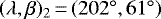 . Curiously, the first pole solution would fit rather well with the originally reported group of Koronis prograde rotators in the Slivan state, but the rotation period is longer.
This new solution for one of the original Slivan targets prompted us to re-evaluate the situation and see if the above-outlined story of Vokrouhlický et al. (2003) still holds. Before we deal with this primary goal (in Sect. 3), we first present the current rotation-state solution for (208) Lacrimosa in more detail (Sect. 2). In particular, to confirm the stability of the solution, we obtained new observations during the last Lacrimosa opposition and added them to the full observational record for this asteroid. Additionally, we included sparse photometric observations from numerous sky surveys and stellar occultations from two different epochs. We then conducted a numerical exploration of its short- and long-term evolution (Sect. 3). Some details of the mathematical methods and numerical tools are summarized in Appendix A. Basic information about our new observations of Lacrimosa are given in Appendix B. Our best-fitting model is compared with all available observations in Appendix C.
2 Rotation state of (208) Lacrimosa
As mentioned above, the spin state of (208) Lacrimosa published by Ďurech et al. (2019) was different from that in Slivan (2002) and Slivan et al. (2003). To ensure that the new pole solution is correct, we repeated the light-curve inversion with a much larger dataset. We collected all available light curves (Binzel 1987; Slivan & Binzel 1996; Stephens 2014) and sparse photometry from Gaia DR2 (Gaia Collaboration 2018), ASAS-SN (All-Sky Automated Survey for Supernovae; Shappee et al. 2014; Kochanek et al. 2017), ATLAS (Asteroid Terrestrial-impact Last Alert System; Tonry et al. 2018), and United States Naval Observatory (USNO) and Catalina observatories downloaded from Minor Planet Center (MPC). We also carried out new photometric observations of Lacrimosa with TRAPPIST-South and TRAPPIST-North telescopes in March and June 2020 (e.g., Jehin et al. 2011). Some technical details of these new observations and their reduction methods are given in Appendix B. All photometric data used for the inversion are listed in Table B.1, and their comparison with the best-fitting model is shown in Appendix C.
2.1 Data analysis and new model for (208) Lacrimosa
From light curves and sparse photometry, we reconstructed two convex shape models with the inversion method of Kaasalainen et al. (2001). One of the models (shown in Fig. 1) has the pole direction (15° ± 2°, 67° ± 2°) in ecliptic longitude and latitude and its rotation period is P = 14.085734 ± 0.000007 h. The second model has the same rotational period, and its pole direction is (204°, 68°). Both models provide the same RMS fit of the data. Because Lacrimosa’s orbital inclination to the ecliptic is only 1.7°, the viewing and illumination geometry of observations is always limited to the ecliptic plane. For that reason, disk-integrated photometry can never distinguish between these two symmetric pole solutions, which have the same ecliptic latitude and ecliptic longitudes that are 180° apart (Kaasalainen & Lamberg 2006). The uncertainty on spin parameters given above was estimated using a bootstrap approach. We created 1000 bootstrapped data sets by randomly resampling light curves and sparse data points and repeated the light-curve inversion. For each resampling, the inversion algorithm converged to a slightly different set of parameters. Their standard deviation served as an estimate of their uncertainties.
The new spin solution is different from that derived by Slivan et al. (2003), which was also used in the original spin-clustering paper by Slivan (2002). These latter authors derived a rotation period of 14.07692 ± 0.00002 h and a retrogradepole solution. Their result was based on a limited data set (see Table B.1), and was apparently only one of several local minima in the parameter space. Indeed, this weakness was noted already by Slivan et al. (2003), who mentioned: “The pole results for Lacrimosa are preliminary and should be checked by further observations; especially needed are a good single-apparition solar phase function and complete light curves at unobserved or incompletely observed aspect longitudes”. Our new analysis with a much larger data set shows that the correct sidereal rotation period is slightly different from that of Slivan et al. (2003). Interestingly, this small discrepancy in periods leads to a dramatic difference in spin axis directions, namely the change from retrograde to prograde rotation.
Our new model is also consistent with thermal infrared (IR) data from for IRAS, Akari, and WISE observatories compiled in the Small Bodies: Near and Far Database (SBNAF, Szakáts et al. 2020), from where we downloaded processed fluxes. We used the approach of Ďurech et al. (2017) and reconstructed a model of Lacrimosa from its light curves combined with thermal data. There were different possibilities for thermophysical parameters that gave similar fits to data, one of them having thermal inertia Γ = 30 J m−2 s−0.5 K−1, geometric albedo pV = 0.20, and volume-equivalent diameter D = 44 km. Its pole direction of (13°, 70°) is close to the value based on photometry alone. Because thermal data were also acquired at plane-restricted geometries, the same symmetry applies here, and both pole directions are equally good in fitting thermal data. Our solution utilizing thermal data is therefore very close to that obtained by Masiero et al. (2011), who obtained D = 45.0 ± 4.6 km and pV = 0.168 ± 0.055.
Finally, there are two stellar occultations by Lacrimosa observed in 2003 and 2016 (Herald et al. 2020). We computed the orientation of our two models for the time of occultations, computed the projected silhouettes, and scaled and shifted the shape models to get the best agreement between the silhouettes and the occultation chords (for details, see Ďurech et al. 2011). Because there were no timing errors reported for the 2003 occultation, we assumed errors of 0.1 and 0.5 s forphotoelectric and visual observations, respectively. Only one positive chord was observed during the occultation in 2016, and so the only constraint comes from the 2003 occultation. The results are shown in Fig. 2. Although the number of chords is not sufficient for any high-fidelity work, the first pole solution (15°, 67°) fits the occultation data better than the second one with pole direction (204°, 68°). The volume-equivalent diameter is 44 ± 2 km for the first model; this diameter is 46 ± 3 km for the second model with much worse formal fit. For comparison, we also show a silhouette of the shape model derived by simultaneous inversion of optical and thermal data.
An important take-away experience from our analysis of Lacrimosa can be summarized as follows. Although further photometricobservations can refine the shape model and increase the accuracy of spin parameters, the pole ambiguity cannot be avoided by any amount of disk-integrated data. The only way to distinguish between the two spin axis directions is through disk-resolved data. For example, a well-observed occultation would enable us to confirm that the (15°, 67°) pole is the correct one. Moreover, it could also help us to constrain the shape more tightly, namely its dynamical ellipticity Δ, which is discussed in the following sections. Nevertheless, because the available occultation data already now favor this first photometricsolution of the pole of Lacrimosa, we consider it a viable solution in what follows.
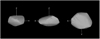 |
Fig. 1 Shape model of Lacrimosa for pole direction (15°, 67°) shown from equatorial level (left and center, 90° apart) and pole-on (right). |
2.2 YORP torques for (208) Lacrimosa
Vokrouhlický et al. (2003) pointed out that modeling of the very long-term evolution of Koronis asteroid spin states requires inclusion of the YORP effect in the dynamical model. We therefore need to estimate its strength. This task is quite troublesome if high precision is required (such as needed for comparison with YORP detections on small near-Earth asteroids; see discussion in Vokrouhlický et al. 2015) but this is not the case here. Our goal is to simply characterize the possible evolution of Lacrimosa’s spins state that would result in its current value. It is not our ambition, and it is not even possible, to hope for any determinism in this task. Therefore, it is adequate to estimate the YORP effect within a factor of a few in accuracy for our purposes.
We used the zero thermal conductivity approach of Vokrouhlický & Čapek (2002), adopted the best-fit, scale-calibrated model of Lacrimosa outlined above (volume-size corresponding to a spherical body of diameter ≃ 44 km), and assumed a bulk density of 2 g cm−3. With the parameters of the present spin state, and the heliocentric orbit, we obtained: (i) the rate of change of the rotational frequency ω equal to d ω∕d t ≃−2.98 × 10⁻⁸ s−1 Myr−1, and (ii) the rate of change of the obliquity ε equal to d ε∕d t ≃−0.014 deg Myr−1 (we did not need to compute the YORP effect on ecliptic longitude, because this contribution is much smaller than the precession due to solar gravitational torque). Both ω and ε are thus predicted to decrease at this moment. The current value of the doubling timescale (e.g., Rubincam 2000) therefore reads |ω∕(d ω∕dt)|≃ 4.16 Gyr. Another way of illustrating the YORP effect is to translate dω∕dt to the present-day rate of change of the rotation period P. If this value is conserved, P will increase by ≃ 3.4 h in the next gigayear. In reality, the effect is even larger, because dP∕dt ∝ P2 for an approximately constant dω∕dt. As P increases, the rate dP∕dt therefore accelerates. The take-away message is that the YORP effect is indeed fully capable of significantly changing Lacrimosa’s rotation period on a timescale of 1 Gyr, which is comparable to the age of the Koronis family.
To enable efficient long-term propagation of spin state with the YORP torques, we also precomputed d ω∕d t and d ε∕d t values for the dense grid in obliquity (using 2° step). In our simulations described in Sect. 3.2 we simply interpolated among these values to obtain d ω∕d t and d ε∕d t for an arbitraryobliquity (see Appendix A.1).
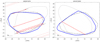 |
Fig. 2 Projections of two occultations from December 31, 2003 (left), and October 20, 2016 (right). Individual observations are shown as straight red lines. Solid lines are photoelectric observations, dashed are visual observations, and dotted are negative observations. Timing errors are displayed as gray strips. The blue solid silhouette is that of the best-fit model, the dotted silhouette is of the second pole solution, and the dashed silhouette is of the IR-based shape model without any scaling. North is up, west to the right. |
3 Theory
The analysis of observations in the previous section provides parameters of the rotation state at the current epoch. It assumes the spin orientation and sidereal rotation rate are constant, at least over the few decades covered by the data. Given the measurement accuracy, this is a justifiable assumption. However, over a longer period of time all rotation-state parameters evolve. Here we pay attention to secular effects, namely those with characteristic timescale longer than the sidereal rotation period of the asteroid and its orbital period about the Sun. We first characterize short-term secular effects (1 Myr timescale; Sect. 3.1). This initial step is important for two reasons. First, its formulation is a little more simple and deterministic, because we may safely neglect inaccurately quantified nongravitational torques. At the same time, the analysis provides us a clear response as to whether the current rotation state of (208) Lacrimosa occupies theSlivan state or not. Equipped with this knowledge, we can then explore possibilities of very long-term evolutionary scenarios for Lacrimosa (1 Gyr timescale; Sect. 3.2), although in this case with less determinism.
3.1 Short-term spin state evolution of (208) Lacrimosa
The sidereal rotation frequency ω is conserved when restricting to the secular effects of the solar gravitational torque. Consequently, the only evolving component of the rotation state is the direction s of the spin vector. As discussed in Appendix A.1, the flow of s on a unit celestial sphere may be understood using the Colombo top model. The orbital precession frequency of interest may be either the forced frequency s6 ≃ −26.34 arcsec yr−1 or the proper frequency s ≃ −67.25 arcsec yr−1. As the flow of s in the prograde-rotating mode is fundamentally affected by the presence of the resonant zone about the Cassini state 2 (“Cassini resonance”), it is useful to first determine whether or not this resonance exists. For a given orbit, such as that of (208) Lacrimosa, and the two possible orbital precession modes, the answer depends on two parameters (more specifically, on their product P Δ): (i) the sidereal rotation period P, and (ii) the dynamical ellipticity Δ. At the current epoch, P is known very accurately. As discussed in the previous section, observations constrain Δ as well, but with a much smaller accuracy.
Figure 3 shows maximum obliquity extension of the Cassini resonance as a function of Δ for two different values of the rotation period: (i) the present value P = 14.085734 h (left), and (ii) a twice that value, P = 28 h (right). The latter may correspond to the situation in the distant future, because we showed that the YORP effect decreases the rotation rate. In the first case, (i), the Cassini resonance exists for the precession mode s6 whenever Δ > Δ⋆ ≃ 0.217. As Δ increases, the location of the Cassini resonance moves to larger obliquity values and its extension slightly decreases. The Cassini resonance related to the proper frequency s does not exist for any value of Δ. In the case of the longer rotation period P = 28 h, (ii), the onset of the Cassini resonance associated with the s6 frequency moves to Δ⋆ ≃ 0.115. This is because for a fixed orbital precession frequency Δ⋆ ∝ P−1. The novel feature consists of bifurcation of the Cassini resonance associated with the s frequency at Δ⋆ ≃ 0.305. This resonance is wider in the obliquity because the proper orbital inclination IP is about four times larger than the forced inclination I6. The s-frequency Cassini resonance appears at low obliquity values at Δ⋆, and is well separated from the s6-frequency Cassini resonance. For Δ > 0.4, on the other hand, the two resonances approach and eventually overlap. The resonance overlap occurs at the Δ value whichis inversely proportional to the rotation period; for instance with Δ ≃ 0.35 the required rotational period is P ≃ 32 h.
Returning to the present rotational configuration of Lacrimosa (left panel of Fig. 3), we now focus on the red symbols: these are just under 1000 solutions described in Sect. 2, all of which correspond to statistically acceptable fits to the observations. The 95% confidence level interval of the obliquity ranges from 19.5° to 26.9°, with the best-fit value of 22.4°. The same confidence-level interval of the dynamical ellipticity is in between 0.30 and 0.39, with the best-fit value of 0.35. There is a slight correlation between these two values, pushing the obliquity to larger values for smaller ellipticity values. The main take-away message here is that only two stray solutions out of 1000 fall into the range of the obliquity values delimiting the Cassini resonance of the s6 orbit precession mode; the majority of the 1000 solutions, including the best-fitting solutions, provide dynamical ellipticity values away from the resonance criterion. Assuming the rotation pole direction (i.e., obliquity) is set accurately enough, the necessary value of the ellipticity Δ would be about 30–35% smaller than the values determined from the shape models. It is highly unlikely that the shape models would be mistaken at this level, or that the internal density would deviate so much from a uniform distribution. Instead, we may preliminarily conclude that the spin state of (208) Lacrimosa is not in the Slivan state.
A more detailed understanding of the situation – leading to the same conclusion – is provided by Figs. 4 and 5. Here, we show output from a numerically integrated spin evolution over the next 2 Myr. Initial data are from the best-fitting solution in Sect. 2, namely (λ, β) = (15.2°, 66.9°) and P = 14.085734 h. Results in Fig. 4 are for dynamical ellipticity Δ = 0.23. This value is incompatible with the shape models fitting the observations, but it is the value that we predict will match the Slivan-state location. Results in Fig. 5 are for the best-fitting dynamical ellipticity Δ = 0.35, and confirm Lacrimosa’s spin misalignment with respect to the Slivan state. We used a full-fledged numerical scheme described in Appendix A.2 in which the secular spin evolution is propagated together with the heliocentric orbital motion. Radiative torques were neglected, which is an approximation that is well justified by the short interval of time described.
The upper panels on both Figs. 4 and 5 show the osculating obliquity as a function of time. The bottom panels show the phase space of the Colombo-top model associated with the s6 precession frequency (see the Appendix A.1): (i) the longitude φ6 (coordinate) reckoned from the direction 90° away from the ascending node Ω6 = s6t + Ω6,0 (with Ω6,0 ≃ 289° in the planetary invariable system and time t origin at J2000.0), and (ii) ε6 (or cosε6 on the left ordinate; momentum) which is the obliquity value in the orbital frame with node Ω6 and inclination I6 ≃ 0.53°. The solid black line in all panels is the result from our numerical propagation. The gray lines in the bottom panels are isolines of the Colombo model first integral (A.11). Because there are more terms contributing to the precession of Lacrimosa’s node, in particular the proper s term, the gray lines serve only as guidelines of the true motion about which the solution oscillates. Two particularly interesting isolines of the first integral are highlighted in red: (i) the separatrix (boundary) of the Cassini resonance, and (ii) the Cassini state 2 (red dot in the center of the resonant zone). The spin evolution described in Fig. 4 confirms what is suggested by Fig. 3, namely that a smaller dynamical ellipticity value Δ = 0.23 would help to locate the spin evolution to the Slivan state. The phase space trajectory librates about the Cassini state 2. The usefulness of representing the secular spin evolution in this coordinate system stems from the fact that the Slivan state dictates the principal features of the motion. In particular, the large-amplitude and long-period oscillation of the obliquity directly reflects libration motion about the resonance center C2. The effects related to the leading term in the orbital plane precession, namely the proper term with frequency s, represent only a small perturbation. This is because the libration period of ≃ 745 kyr is an order of magnitude longer than any of the periods of significant terms characterizing the precessional motion of the orbital plane in space.
However, the observations support a different behavior depicted by Fig. 5. In this case, the Cassini resonance is displaced to larger obliquity and the true evolutionary path of Lacrimosa’s spin simply circulates about the Cassini state 1 (phase space representation in Fig. 5 is not suitable to show the location of this center, which maps onto obliquity ε6 ≃ 0.73° and φ6 = ±180°). The osculating obliquity of Lacrimosa (top panel) shows a simple oscillatory behavior with an amplitude of ≃ 6.5°. This value is larger than the obliquity oscillation related to the motion about the C1 center and is even larger than the proper inclination IP ≃ 2.15° of Lacrimosa’s orbit. In fact, it is entirely forced by the obliquity of the Cassini state 2 related to the orbital plane precession mode with proper frequency s (see left panel of Fig. 3).
In order to better understand this effect, we also re-mapped the numerically determined spin evolution of Lacrimosa to the coordinates of the phase space of the Colombo-top model associated with the s precession frequency. This is shown in the bottom panel of Fig. 6. The numerically integrated trajectory of Lacrimosa’s spin now more closely follows isolines of the Colombo model first integral (A.11), which means the spin evolution is more conveniently represented in these coordinates. The effects due to the s6 precession mode in the orbital plane evolution produce only a very small perturbation. The Cassini state 2 (red symbol in Fig. 6) has an obliquity of ≃6.5° and its presence triggers the whole amplitude of the obliquity evolution. The period of the osculating obliquity oscillations, ≃ 53 kyr, is just the period of spin vector circulation about the Cassini state 2.
We conclude this section by observing that the present-day spin state of (208) Lacrimosa is not in the Slivan state despite its prograde sense of rotation. In this respect its behavior differs from that of the other Koronis family asteroids in this size range. How this is possible, and its implications for the very long-term evolution of the spin state of this asteroid are investigated in the following section.
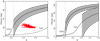 |
Fig. 3 Obliquity ε2 of the Cassini state 2 as a function of the dynamical ellipticity Δ (see Eq. (A.3)). Orbital parameters of (208) Lacrimosa are assumed. Left panel: nominal rotation period P = 14.085734 h of (208) Lacrimosa used. The solid line labeled C2(s6) provides ε2 for the s6 (forced) frequency mode of the nodal precession. The spin-orbit resonance onsets for Δ are denoted by the light-gray dashed line (transition determined by the Eq. (A.7) condition); beyond this value the Cassini state 2 becomes an equilibrium point of the spin-orbit resonance,whose maximum extension in obliquity is shown by the gray area. Solid line labeled C2 (s) provides ε2 for the s (proper) mode of the nodal precession. Here the spin-orbit resonance does not exist. Red symbols show obliquity and Δ values for a little less than 1000 solutions for (208) Lacrimosa from the bootstrap method discussed in Sect. 2 and using only the optical light-curve observations. The blue star is the nominal, best-fit solution. Right panel: same as in the left panel, but now for a hypothetical, longer rotation period of P = 28 h. Now the spin–orbit resonance exists beyond some critical Δ value for both frequencies s6 and s. |
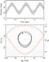 |
Fig. 4 Top panel: time evolution of the osculating obliquity ε for (208) Lacrimosa over the 2 Myr interval using numerical integration of Eq. (A.1) with Tng = 0. The initial conditions at the present epoch from the best-fit rotation state solution (P = 14.085734 h, λ = 15.2° and β = 66.9°) and Δ = 0.23. The short-period oscillations are due to the proper term of nodal precession with frequency s (which have a period of ≃2π∕(s − s6) ≃ 32 kyr). The long-period and large-amplitude oscillations of ≃745 kyr are due to libration about the resonant Cassini state 2 associated with frequency s6 (“the Slivan state”). Bottom panel: phase portrait of the Colombo top model for the s6 frequency and precession constant α ≃ 29.75 arcsec yr−1 (i.e., P = 14.085734 h and Δ = 0.23 in Eq. (A.4)); the ordinate is either cosε6 (left) or ε6 (right) and the abscissa is φ6. The light-gray curves are isolines of the first integral C(ε6, φ6) = constant given by Eq. (A.11). Critical curves of the spin-orbit resonance, namely the separatrix and the stable equilibrium C2, are highlighted in red. The black curve is the numerically integrated pole of (208) Lacrimosa from the top projected into the plane of these variables; the blue diamond is the current position of the pole. |
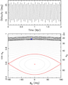 |
Fig. 5 Top panel: time evolution of the osculating obliquity ε for (208) Lacrimosa over the 2 Myr interval using numerical integration of Eq. (A.1) with Tng = 0. The initial conditions at the present epoch from the best-fit rotation state solution (P = 14.085734 h, λ = 15.2° and β = 66.9°) and Δ = 0.35. The amplitude of the oscillations, which is larger than the proper inclination (≃ 2.15°), is forced by the Cassini state 2 of the s frequency at ≃6.5° (see Fig. 3). Bottom panel: phase portrait of the Colombo top model for the s6 frequency and precession constant α ≃ 45.27 arcsec yr−1 (i.e., P = 14.085734 h and Δ = 0.35 in Eq. (A.4)); the ordinate is either cosε6 (left) or ε6 (right) and the abscissa is φ6. The light-gray curves are isolines of the first integral C(ε6, φ6) = constant given by Eq. (A.11). Critical curves of the spin-orbit resonance, namely the separatrix and the stable equilibrium,are highlighted in red. The black curve is the numerically integrated pole of (208) Lacrimosa from the top projected into the plane of these variables; the blue diamond is the current position of the pole. |
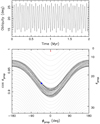 |
Fig. 6 Same as in Fig. 5, but here the bottom panel shows phase space coordinates of the Colombo top model for the s frequency. As shown in Fig. 3, the Cassini resonance does not exist and the Cassini state 2 has an obliquity of ≃ 6.5° (red point). Lacrimosa’s spin vector circulates about C2 (black line) and follows the isolines of the first integral (A.11) more closely than in Fig. 5. |
3.2 Possible long-term evolution of the rotation state of (208) Lacrimosa
Vokrouhlický et al. (2003) noted that many but not all initial conditions of possible long-term evolution scenarios resulted in the Slivan-state situations reported by Slivan (2002). Vokrouhlický et al. (2003) showed the positive cases (e.g., Fig. 1 in their paper) but only commented on the negative cases. For obvious reasons, we are now interested in the opposite situation.
The initial data suitable for capture in the Slivan state had the following common properties (see Vokrouhlický et al. 2003): (i) the YORP evolution asymptotically decelerated the rotation of the asteroid, and (ii) the initial rotation period was smaller than ≃ 7 h. If these conditions were satisfied, the initial obliquity had only to be positive, but was not restricted otherwise. The generic evolution first made the obliquity reach a small value due to the YORP torque, while still keeping the rotation period short enough. As a result, the precession frequency αcosε from Eq. (A.2) along this evolutionary path remains smaller than the − s6 frequency. Only when the rotation period increases sufficiently does the resonant condition α ≃−s6 for small obliquity values become satisfied (this is because α ∝ P, Eq. (A.2)). At the same time, the capture into the resonance is guaranteed (i.e., 100% probable) as long as the resonant condition occurs when the instantaneous obliquity is ≤ 20°, a comfortably large value. Once captured in the Slivan state, the continuing increase in the rotation period due to the YORP effect only makes the Cassini resonance drift toward a larger obliquity, which eventually approaches ε ≃ 50°−55° where the YORP-driven period evolution stalls. We note that the spin state follows this evolution adiabatically, because the characteristic timescale of the YORP-driven changes is much longer than the libration period about the Cassini state.
What happens in the situation where (i) in the above paragraph is satisfied, but (ii) is not satisfied (i.e., the initial rotation period is longer)? An example of such evolution is shown in Fig. 7. In this case, we assume P = 12.25 h and ε = 70° initially, and let the evolution proceed with the YORP torques characteristic of Lacrimosa, i.e., body of D ≃ 44 km size and 2 g cm−3 bulk density. We used Δ = 0.35, which is Lacrimosa’s nominal value of dynamical ellipticity (Fig. 3). The initial phase of the evolution resembles what has been described above: the YORP torque causes the obliquity to decrease, while the rotation period evolves slower (this is because near ε ≃ 55° the rotation period change due to YORP is nil). However, the main difference is that already the initial value of the spin axis precession rate α cosε is faster than − s6 because of the larger P value. At about 1.45 Gyr, the resonance condition αcosε ≃−s6 becomes satisfied. At this moment, the mean obliquity is still large – about 50° – and the resonance has been approached from the zone of larger obliquity values (rotation pole circulating about the Cassini state C3). The adiabatic capture theory described in Appendix A.1 (see also Henrard 1982) allows us to estimate the capture probability. Using Eqs. (A.12) and (A.13) we find this probability is zero (see Fig. 9). Indeed, the numerically propagated spin of Lacrimosa jumped over the resonance and continued evolving toward smaller obliquity while the rotation period increased due to the YORP torques. At ≃ 2.4 Gyr, the possible age of the Koronis family (e.g., Nesvorný et al. 2015), the simulated obliquity and rotation period closely resemble those of Lacrimosa. In this view, the lack of Lacrimosa’s pole residence in the Slivan state is naturally explained by avoiding a capture in the first place.
For the sake of interest, we continued our simulation until 6 Gyr, allowing us to predict what may possibly happen to Lacrimosa’s spin state in the future. At about 2.8 Gyr, the simulated spin starts to closely follow the Cassini state C2 associated with the proper orbital frequency s. At small obliquity values, the rotation period continues to decrease and at about 4.1 Gyr, when P ≃ 24.4 h, the Cassini resonance of this frequency bifurcates (see also right panel on Fig. 3, which applies to only slightly larger rotation period of 28 h). From that epoch, the modeled spin state becomes locked in the new Slivan (resonant) state, but this time associated with the proper frequency. Because the proper frequency s is larger than s6, the required rotation period is longer. The evolution follows the pattern known from the theory of classical Slivan states in Vokrouhlický et al. (2003), namely a long-term increase in the obliquity and rotation period. Finally, at about 5.63 Gyr the amplitude of obliquity oscillation starts to increase. This is associated with the increase in the amplitude of oscillation of the resonant libration angle (bottom panel at Fig. 7). This phase of evolution is triggered by an overlap of the Cassini resonances associated with the s6 and s orbital frequencies, which were separated until that moment.
An interesting intermediate case of possible long-term spin evolution is shown in Fig. 8. We kept the same initial conditions, and other parameters, as above (Fig. 7, except for the shorter initial rotation period of P = 9 h to expect a regular evolution that would result in a capture in the Slivan state, Vokrouhlický et al. 2003). Because of the shorter P value in the initial phase of the evolution, the resonance condition αcosε ≃−s6 is now met in the situation where obliquity ε has already evolved to a smaller value of ≃20°. As a consequence (see Fig. 9), the capture in the Slivan state is possible at ≃ 2.25 Gyr. However, the condition is just barely satisfied and the capture results in a large-amplitude libration situation about the Cassini state C2. Subsequently, the evolution takes the usual direction towards larger obliquity while being characterized by the Slivan state capture. However, the large-amplitude libration state is susceptible to instability, and the spin state is released from the resonance followed by an interval of time dominated by YORP torques, during which the obliquity again migrates toward the smaller value. At ≃5.85 Gyr, the obliquity and rotation period match those of Lacrimosa. Obviously, this cannot be accepted as a satisfactory history for this object, because the needed timescale is longer than the age of the Solar System. However, smaller members in the Koronis family with a similar rotation state as in (208) Lacrimosa, such as (263) Dresda, could take the evolutionary path described in Fig. 8. This is because, for them, the YORP torques are stronger and the associated characteristic timescale of evolution scales ∝ D2. Therefore, with a size of about 26 km, Dresda’s spin evolves due to YORP about 2.8 times faster.The 5.85 Gyr then recalibrates to ≃2.1 Gyr, plausible for the Koronis family age (we note that this is obviously just a size-scale argument, because the shape of Dresda may lead to YORP torques of somewhat different strength). While these details are important for specific cases, they do not invalidate a general conclusion that some smaller members (say, 15− 25 km in size) in the Koronis family might have undergone the spin evolution depicted in Fig. 8. The interesting difference from larger objects consists of the past capture in the Slivan state, but later evolution away from it. This is especially expected to happen among the smaller Koronis members for which the YORP torques are stronger. The take-away message is that as the spin states of the smaller members of the Koronis family become known in the future, we may expect more cases unrelated tothe Slivan pattern seen in the population of the larger Koronis objects (Slivan 2002). It is interesting to note that the spin evolution shown in Fig. 8 evolves also to the capture in the Slivan state associated with the s rather than s6 frequency. As a result, we may also expect the future spin-state solutions for small Koronis members to bring evidence of this configuration.
For sake of completeness we mention that numerical tests with initial rotation period larger than 16 h did not lead to configurations that would match Lacrimosa’s rotation parameters in 2− 4 Gyr.
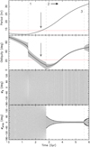 |
Fig. 7 Example of a possible long-term evolution of the rotation state for (208) Lacrimosa. Rotation period P (top), osculating obliquity ε (middle-up),and longitude φ in the orbital frame associated with the s6-frequency and s-frequency term of the nodal precession (middle-down and bottom; note φ is measured from an axis 90° away from the corresponding nodal line). The gray dots are densely output osculating values (with a time-step of 5 kyr). Black symbols in the obliquity panel are average values in a 2 Myr running window; black symbols in the bottom panels are maximum and minimum values of the respective longitude in a 2 Myr running window. The dynamical model uses solar gravitational torque and the YORP effect with parameters determined from the best-fitting solution in Sect. 2. The red lines in the upper two panels show the present state of (208) Lacrimosa for reference. At the epoch of ≃ 2.4 Gyr, the propagated spin evolution roughly matches the present state (as indicated by the gray arrows). At ≃ 1.45 Gyr (verticaldashed line 1), the solution jumps over the Slivan state of the s6 precession frequency, where other large Koronis prograde-rotating asteroids are located. At ≃ 2.8 Gyr (vertical dashed line 2), the solution starts to closely follow the Cassini state 2 associated with the s precession frequency. This is allowed by (i) the low obliquity (where C2 is located), and (ii) the increasing rotation period. The Cassini resonance formally bifurcates when the rotation period reaches ≃24.4 h, i.e., at ≃4.1 Gyr. Finally, at ≃5.63 Gyr (vertical dashed line 3), the small-amplitude oscillations about the resonant Cassini state 2 in the s precession frequency frame become perturbed by an overlap with the Cassini resonance associated with the s6 precession frequency. The simulations had an initial rotation period of 12.25 h and an initial obliquity of 70°. |
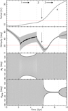 |
Fig. 8 Same as in Fig. 7, but now for a different initial rotation period of 9 h. In many respects, the evolution is similar to that shown in the previous figure with one important exception: at ≃ 2.25 Gyr (vertical dashed line 1) the spin state becomes captured in the Slivan state of the s6 precession frequency; it remains located in the Slivan state until ≃5 Gyr (verticaldashed line 2), when the amplitude of resonant libration grows to 180°. Consequently, the spin state leaves the Slivan state and continues to evolve primarily by YORP torques: the obliquity drifts to small values and the rotation period slowly increases; at ≃ 5.85 Gyr (highlighted by the arrows), both roughly match the current values of (208) Lacrimosa. As the rotation period continues to grow, the spin evolution follows the trend seen also in Fig. 7: it starts to closely follow the Cassini state 2 associated with the s precession frequency (eventually becoming captured in the corresponding Slivan state). |
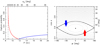 |
Fig. 9 Left panel: capture probability to the spin-orbit resonance in a Colombo top model with an adiabatically slow change in the asteroid rotation period P (at the abscissa). Heliocentric orbit of (208) Lacrimosa, dynamical ellipticity Δ = 0.35, and s6 mode of the orbital node precession were used. With these assumptions, the resonance bifurcates at ≃ 8.73 h rotation period (vertical dashed line). The red line indicates probability P+ of a capture from orbits originally circulating about the Cassini state C3, the blue line indicates probability P− of a capture from orbits originally circulating about the Cassini state C1. The analytical theory of Henrard & Murigande (1987) is briefly recalled in the appendix; see Eqs. (A.12) and (A.13). The upper abscissa shows obliquity ε2 of the Cassini state C2, the equilibrium point of the resonance. Right panel: phase portrait of the Colombo top for rotation period P = 14.085734 h (other parameters as above). The gray curves are isolines of the integral C(ε, φ) = constant given by Eq. (A.11). The black curve is the separatrix and the black dot shows the location of the Cassini state C2. The arrows schematically indicate the capture in the resonance from orbits originally circulating about the Cassini state C1 (blue) and C3 (red); in a model where only the rotation period P slowly changes, the former occurs for a decrease in P and the latter occurs for an increase in P. |
4 Conclusions
In this paper, we present new observations of asteroid (208) Lacrimosa, one of the largest members of the Koronis family. When joining these new data with the previously available photometric dataset, we confirm (and improve) the rotationstate solution obtained earlier by Ďurech et al. (2019). Unlike in Slivan (2002), the rotation of Lacrimosa is found to be prograde. While Ďurech et al. (2019) still had two possible pole solutions separated by 180° in the ecliptic longitude, here we find that stellar occultation data allow one of them to be favored. Our analysis indicates a rotation period of P = 14.085734 ± 0.000007 h and a pole direction in ecliptic longitude and latitude of (λ, β) = (15° ± 2°, 67° ± 2°). Thermal and occultation data also effectively constrain Lacrimosa’s volumic size to D = 44 ± 2 km, in good agreement with a previous solution based on WISE observations.
Large asteroids in the Koronis family, when in prograde rotation, were found to be locked in the Slivan state (e.g., Slivan 2002; Vokrouhlický et al. 2003). Therefore, we analyzed Lacrimosa’s status with respect to this configuration. We find that Lacrimosa’s spin may well be confined to the Slivan state provided the value of the dynamical ellipticity Δ is in the range ≃ (0.22–0.26). However, our convex shape models obtained from the light-curve inversion analysis result in larger values, namely Δ ≥ 0.28. The bootstrap approach to the observation fit helps us to constrain Δ to 0.35 ± 0.05. Therefore, we conclude that Lacrimosa’s rotation pole does not reside in the Slivan state: in other words, its dynamical ellipticity is too large or its obliquity too small for the rotation pole to be in the Slivan state (Fig. 3).
We then sought a reason as to why Lacrimosa is different in this respect from other large Koronis asteroids rotating in a prograde fashion. The easiest solution we find consists in the assumption that the initial rotation period of Lacrimosa was slightly longer, notably in the range of 11 to 15 h. For those values, and initial obliquity larger than ≃50°, we find that spin evolution avoids capture in the Slivan state. Instead, it typically reaches the Cassini resonance condition at a still too high obliquity value and consequently jumps over the Slivan state. Further evolution toward a small obliquity value explains the current spin configuration of Lacrimosa. Our numerical simulations also suggest that Koronis members with slower rotation are efficiently captured in the Slivan state associated with the proper mode s of the orbital precession, instead of the forced mode s6 (the classical Slivan state).
One of the main purposes of this paper is also to highlight an expected diversity of spin states among the small asteroids in the Koronis family. While the large members of this family generally follow the Slivan-state paradigm (Slivan 2002; Vokrouhlický et al. 2003), small members – for which the YORP torques are stronger – may evolve further. Their possible past Slivan states might already have been destabilized, allowing evolution to longer rotation periods and small obliquities. If pushed even further, a new type of Slivan state, namely capture in the Cassini resonance associated with the s precession frequency of the orbits, is also expected. Some other evolutionary paths may also entirely avoid capture in the traditional Slivan state by jumping over the Cassini resonance. In summary, small Koronis members should exhibit a much larger variety of spin states than would be expected from the Slivan sample of large members. The forthcoming data from future large-scale surveys will allow this conclusion to be tested.
Acknowledgements
This research was supported by the Czech Science Foundation: the work of DV through grant 21-11058S, the work of JĎ and JH through grant 20-08218S. The work of J.H. has been also supported by the INTER-EXCELLENCE grant LTAUSA18093 from the Czech Ministry of Education, Youth, and Sports. TRAPPIST is a project funded by the Belgian F.R.S.-FNRS under grant FRFC 2.5.594.09.F. TRAPPIST-North is a project funded by the University of Liège, in collaboration with the Cadi Ayyad University of Marrakech (Morocco). E. Jehin is a FNRS Senior Research Associate.
Appendix A Methodsand numerical tools
In this appendix, we provide a brief overview of the mathematical formulation and numerical tools needed for description of an asteroid’s rotation state over long periods of time. This has become a classical chapter of celestial mechanics, and so we mostly refer to previous publications, where more detailed calculations were performed.
A.1 Theory
Rotational angular momentum L of an asteroid evolves as a response to external torques of both gravitational Tg and nongravitational Tng origin. Aiming to describe long-term evolution of L, we assume Tg and Tng are averaged over rotation and orbital timescales. For sake of simplicity, we also assume the asteroid rotates about the shortest axis of the inertia tensor (appropriate for cases discussed in this paper), therefore L = Cω s with C the largest principal value of the inertia tensor, ω the rotation frequency, and s the unit vector specifying direction of L. The gravitational part Tg is dominated by the effect of the Sun, in particular quadrupole representation of its tidal field at the location of the asteroid (higher-multipole contributions and those from planets may be safely neglected). The nongravitational part Tng is due to the YORP effect. In this model, the gravitational torque may be expressed using a simple analytical formula (e.g., Bertotti et al. 2003). Analytic approaches for the YORP torques are also available (e.g., Nesvorný & Vokrouhlický 2007, 2008; Breiter & Michalska 2008), but they are not practical for our purposes. Rather, we use an averaged representation of a numerical work presented in Čapek & Vokrouhlický (2004). With all these assumptions adopted, the Euler equation describing secular evolution of L reads
![Mathematical equation: \begin{equation*} \frac{\textrm{d}\vec{L}}{\textrm{d}t}\,{=}\,{-}\left[\alpha \left(\vec{c}\cdot\vec{s}\right) \vec{c}+\vec{h}\right]\,{\times}\,\vec{L}+\vec{T}_{\textrm{ng}} ,\end{equation*}](/articles/aa/full_html/2021/05/aa40585-21/aa40585-21-eq3.png) (A.1)
(A.1)
with the first term on the right-hand side being essentially the gravitational torque.
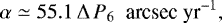
Let us first briefly focus on the effects due to the gravitational torque (hence, for a moment assuming Tng = 0). Referring L to the inertial space would imply h = 0 and  , where I and Ω are inclination and longitude of the node of the asteroid’s heliocentric orbit. The precession constant α reads
 (A.2)
(A.2)
where  , e is the orbital eccentricity, n is the orbital mean motion, and Δ is dynamical ellipticity of the body defined as
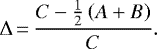 (A.3)
(A.3)
Here (A, B, C) (A ≤ B ≤ C) are the principal values of the inertia tensor. It is useful to note that for the low-eccentricity orbits in the Koronis family (a ≃ 2.89 au and e ≃ 0.05) we have (e.g., Vokrouhlický et al. 2006)
 (A.4)
(A.4)
where P6 = P∕6 h is the rotation period P expressed nondimensionally in units of 6 h (characteristic of many asteroids). The value of Δ is restricted to the interval (0, 0.5), with most typical values between 0.2 and 0.4 for small asteroids (e.g., Vokrouhlický & Čapek 2002).
An alternative to the above-described choice is to refer components of L to the axes comoving with the heliocentric orbital frame of the asteroid (e.g., Bertotti et al. 2003; Breiter et al. 2005). In this case, c takes a trivial form, namely cT = (0, 0, 1), but now 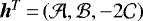 , with
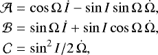 (A.5)
(A.5)
where overdots mean time derivatives. In fact, this latter term −h × L in Eq. (A.1) is not of gravitational origin, but purely induced by transformation to the noninertial, comoving orbital frame.
In either choice, the gravitational torques alone conserve rotation frequency ω and change the spin direction s only. If the heliocentric orbit was fixed in the inertial space (i.e., I and Ω constant, in particular), s would perform a simple precession about c with a frequency 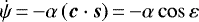 . This notation comes from a traditional representation of s in the orbital frame using
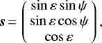 (A.6)
(A.6)
where ε is the obliquity and ψ the precession angle (e.g., Breiter et al. 2005).
However, things are more complicated in reality. In our context of secular spin evolution, this is mainly because the heliocentric orbital plane is not fixed in the inertial space. On the contrary, the planetary perturbations produce its complicated evolution which is reflected in time dependence of I and Ω. It is convenient to merge this information into a complex and nonsingular variable, ζ = sinI∕2 exp(ιΩ). This is because ζ may be represented to an acceptable level of approximation with a finite number of Fourier terms, namely ζ(t) = ∑ Ak exp(ιΩk), each of which has a constant amplitude Ak (i.e., associated inclination value Ak = sinIk∕2) and frequency  (therefore Ωk = skt + Ωk,0). A typical spectrum of frequencies sk for an asteroid consists of (i) a proper mode, associated with free initial conditions of the orbital motion and denoted by s, and (ii) forced modes, imprinted from the perturbing planets (additionally, terms with frequencies given by linear combinations of s, and planetary frequencies may also contribute). The forced terms are dominated by effects of giant planets denoted by s6, s7 and s8. Their numerical values are s6 ≃−26.34 arcsec yr−1, s7 ≃−2.99 arcsec yr−1 and s8 ≃−0.69 arcsec yr−1 of consecutively decreasing frequency (e.g., Laskar 1988). As the s6-related term reflects primarily perturbations by the gas giants, Jupiter and Saturn, its amplitude I6 is the largest. As an example, in the case of (208) Lacrimosa we have I6 ≃ 0.53°, while the proper term has IP ≃ 2.13° and s ≃−67.25 arcsec yr−1. All other terms in Fourier representation of ζ have amplitudes at least an order of magnitude smaller. In the first approximation, we may therefore assume representation of ζ with only two Fourier terms, namely (i) the proper term, and (ii) the forced term with the s6 frequency.
The core of complexity related to the moving orbital plane arises from the fact that the above-mentioned precession frequency  may enter into a resonance with some of the frequencies sk in the Fourier representation of ζ. The nature of this resonance is best explained in a model where ζ is represented with only one Fourier term. In our application of asteroids in the Koronis family, the more realistic situation with two terms in ζ may be understood at the zero order as a high-frequency (s) perturbation of the single-term model with the lower-frequency (s6), or vice versa. This works well especially when the two frequencies, s6 and s, are well separated.
The single-term model for ζ is very useful because of its integrability. This model has been extensively studied and it is known as a Colombo top problem (e.g., Colombo 1966; Henrard & Murigande 1987; Saillenfest et al. 2019; Haponiak et al. 2020). Here we provide its most important features relevant to our study.
We assume that ζ = sinI∕2 exp[ι(st + ϕ)], namely the orbital plane has a constant inclination I and a node precessing with constant frequency s. The most interesting features of the Colombo top derive from occurrence of stationary solutions. Their number depends on a nondimensional parameter κ = α∕(2s). In a simpler situation, when |κ| < κ⋆, there exists two stationary solutions, otherwise there are four stationary solutions (astronomical tradition has it that we call them Cassini states). The threshold value for κ reads (e.g., Henrard & Murigande 1987; Haponiak et al. 2020)
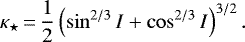 (A.7)
(A.7)
For low-inclination cases,  , and the two new stationary solutions bifurcate when α ≃−s. While stationary with respect to the (moving) frame with nodal longitude Ω = st + ϕ, the Cassini states obviously regularly precess in the inertial space. Their obliquity value is given by solutions of the equation
 (A.8)
(A.8)
with the upper sign − for φ = 0° and lower sign + for φ = 180°; the definition of the longitude in the moving frame is φ = −(ψ + Ω) and it reckons from a direction 90° away from the ascending node (interestingly, the values of cosε for the Cassini state may be obtained analytically as roots of a quartic equation derived easily from (A.8); see, e.g., Saillenfest et al. 2019; Haponiak et al. 2020). Of particular interest is φ = 0° stationary point when |κ| > κ⋆ which is usually referred to as the Cassini state 2 (C2). This is because it has a character of a stable resonant state: small perturbations make obliquity oscillate about ε2 and longitude φ librate about zero (see lower panel on Fig. 4). The nature of the resonance is seen from (A.8) whose limit for I ≃ 0 becomes κ sin2ε ≃−sinε. The obvious solutions ε1 ≃ 0° and ε3 ≃ 180° correspond to the Cassini states 1 and 3 (to be denoted C1 and C3), while the Cassini states 2 and 4 are at approximately αcosε2,4 ≃−s. The left-hand side is the regular precession of s produced by the gravitational torque of the center, while the right-hand side is the orbital precession rate. Thus the Cassini-state 2 resonance expresses 1:1 commensurability between the two. Together with the Cassini-state 4 (C4), C2 form stable and unstable equilibria of the spin-orbit resonance. The maximum width Δε of the resonantzone associated with the Cassini state 2 may be determined from (e.g., Henrard & Murigande 1987; Ward & Hamilton 2004; Vokrouhlický et al. 2006; Saillenfest et al. 2019; Haponiak et al. 2020)
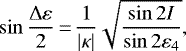 (A.9)
(A.9)
where ε4 is the obliquity of the unstable equilibrium from Eq. (A.8). Alternatively, one can also use somewhat simpler
 (A.10)
An important implication of the square-root factor on the right-hand side of (A.9) or (A.10) is that Δε may be significant (e.g., tens of degrees) even for very small values of I (e.g., a degree); see Fig. 3 for specific examples. Another useful aspect of integrability of the Colombo top problem is the existence of the first integral of motion,
 (A.11)
Conservation of C(ε, φ) allows us to easily represent solutions in the obliquity (ε) versus longitude (φ) plane such as those shown on Fig. 4. Critical points of the surface C(ε, φ) = constant are obviously the above-mentioned stationary points; in the more interesting case of a set of four: (i) the minima specify location of C1 and C3, (ii) C2 is the maximum, and (iii) C4 is the saddle point.
When some of the parameters of the Colombo top model vary slowly in time, C(ε, φ) is not strictly constant. Rather, the system slowly drifts among solutions approximately conserving this parameter. A special situation happens when the motion approaches the separatrix of the spin–orbit resonance. At this moment, the future evolution may either (i) avoid the resonance and continue to circulate about either C1 or C3 equilibrium states, or (ii) it may be captured in the resonance (thus librating about the Cassini state C2). The process is inherentlychaotic (unpredictable). Nevertheless, in an adiabatic model it can be approached probabilistically (e.g., Henrard 1982). Surprisingly, all necessary algebra may be carried out analytically in the Colombo top model (e.g., Henrard & Murigande 1987). Assume, as an example, the rotation period of an asteroid slowly changes. This is reflected in a slow change of the precession constant α in Eq. (A.2). Following the elegant formulation in Henrard & Murigande (1987), one can determine resonance capture probability P+ of a transition from the solution circulating about C3 (see the sense of the red arrow in Fig. 9) and resonance capture probability P− of a transition from the solution circulating about C1 (see the sense of the blue arrow in Fig. 9). In fact, both may be given using a compact formulation:
 (A.12)
where
![Mathematical equation: \begin{eqnarray*} \Psi &\,{=}\,& \frac{4}{\pi}\, \Biggl\{\arcsin \left[\frac{\tan (\Delta\varepsilon/4)} {\tan\varepsilon_4}\right]\\ & & - 2\, \frac{|\kappa|\sin (\Delta\varepsilon/4)}{\cos I} \sqrt{\sin^2 \varepsilon_4 - \sin^2(\Delta\varepsilon/4)}\Biggr\}. \nonumber \end{eqnarray*}](/articles/aa/full_html/2021/05/aa40585-21/aa40585-21-eq22.png) (A.13)
(A.13)
In our context, the rotation period of an asteroid is changed by the YORP effect (Eq. (A.14)). However, the above-given results are only approximate. This is because the YORP effect directly changes also the obliquity (Eq. (A.15)), namely one of the active variables in the Colombo top model. Hence, results from numerical simulations are needed to verify the capture probabilities given above.
The symplectic numerical scheme of Breiter et al. (2005) allows, aside from quadrupole solar torque, to include a general weak dissipative torque T. In our case, T = Tng represents the YORP effect. A distinctive feature of the YORP effect is its ability to change the rotation rate of the asteroid in the long term. This is associated with the nonzero along-spin component of the torque, namely (see Eq. (A.1)),
 (A.14)
The YORP effect also acts on s, in particularobliquity ε and precession angle ψ (e.g., Eqs. (5)–(8) in Čapek & Vokrouhlický 2004). However, the latter represents only a small perturbation compared to the effect produced by the gravitational torque. Therefore, we neglect this component and include the YORP effect on obliquity only:
 (A.15)
(we note that this is conveniently the third component of s in our representation by Eq. (A.6)). Because in this work we aim to illustrate the likely processes in the Koronis family, we do not need highly accurate determination of the YORP effect. We consider the YORP strength determined for the nominal (best-fit) model of Lacrimosa from Sect. 2. Instead of computing YORP torque for a spin-orbit configuration at a given moment during the numerical simulation, we follow the approach of Vokrouhlický & Čapek (2002) and Čapek & Vokrouhlický (2004). In particular, we pre-computed values of the factors (Tng ⋅s)∕C and  on the right-hand side of Eqs. (A.14) and (A.15) as a function of obliquity ε (we note the basic YORP theory does not assume them to be a function of ω). We used a sufficiently dense grid of two degrees in obliquity (see Sect. 2.2). When performing our long-term spin simulations we simply interpolated these rotation-rate and obliquity YORP torques.
A.2 Numerical implementation
We implemented the algorithm developed in Breiter et al. (2005) to numerically integrate Eq. (A.1) (in particular, we use their LP2 splitting scheme). In our approach, the components of L are represented with respect to the frame comoving with the heliocentric orbit. As we deal with secular evolution of L, we may use a long-enough time-step of 50 yr. In addition to initial conditions and dynamical ellipticity Δ as the only external parameter, the code needs information about the orbital evolution due to planetary perturbations. To that end we use two methods.
In the first, more detailed method used in Sect. 3.1, we determine osculating orbital parameters, in particular semimajor axis a, eccentricity e, inclination I, and longitude of node Ω (all needed in Eq. (A.1)), using direct numerical integration of the asteroid’s heliocentric motion. For that purpose we adapted the widely known and well-tested integration package4 swift. Because swift integrates the full system of equations of motion for both planets and asteroid(s) it requires an accordingly short time-step. We used 3 days, short enough to realistically describe orbital evolution of all bodies (including planet Mercury). Initial orbital state vectors for the chosen asteroids and a given epoch were taken from the AstDyS internet database5. and for the planets from the JPL DE405 ephemerides file. To organize the propagation efficiently, we embedded our secular spin integration scheme into the swift package. This arrangement not only allows to propagate the spin evolution online, avoiding large outputfiles with the orbital evolution, but also allows to simultaneously propagate the spin evolution of more asteroids or parametric variants of the same asteroid (for instance testing evolution for different values of the dynamical ellipticity parameter Δ). We note that the spin propagation only needs at a given time to know the orbital parameters in the neighboring grid points in time, which are readily provided by the swift integrator.
The above-mentioned implementation is very precise and has been used for short-term tests such as those shown on Figs. 4–6. However, it is unnecessarily detailed for the propose of very long-term simulations, where our goal is to demonstrate the possible evolutionary tracks of Lacrimosa’s spin state over very long timescales (Sect. 3.2, e.g., Figs. 7 and 8). This is because the implementation based on swift code requires a rather short time-step of the order of days. Therefore, to fully profit from a possibility of a longer time-step (order of years or so) for the propagation of L, we also adopted an approximate variant where the heliocentric orbit evolution was simplified. This means the semimajor axis and eccentricity were assumed constant (and equal to the proper elements of the asteroid), and ζ was represented with two Fourier terms, namely the proper term and the s6 -frequency term (as discussed above). In this case, we also adopted our simplified approach to the YORP effect, namely interpolating the rotation-rate and obliquity torques precomputed using the shape model of Lacrimosa (see Sect. 2.2). For this task, we wrote our own numerical code that implements spin propagator described in Breiter et al. (2005).
Appendix B Observations using TRAPPIST system
TRAPPIST-North (TN) and -South (TS) are 0.6-m Ritchey-Chrétien robotic telescopes operating at f∕8 on German equatorial mounts (Jehin et al. 2011). TN is located at the Oukaimeden Observatory in Morocco (Z53) and the camera is an Andor IKONL BEX2 DD (0.60′′/pixel, 20′ × 20′ field of view). TS is located at the La Silla Observatory in Chile (I40) and the camera is a FLI ProLine 3041-BB (0.64′′/pixel, 22′ × 22′ field of view). We observed Lacrimosa in 2020 using the Johnson–Cousins Rc filter in March and June and obtained dense lightcurves at solar phase angles of ~19° and ~7° respectively (Table B.1). The images were first calibrated with IRAF scripts using the corresponding flat fields, bias, and dark frames. The differential photometry was then performed using Python scripts by selecting nonvariable comparison stars with high S/N and by testing various aperture sizes.
The complete list of the observations available for (208) Lacrimosa, including the new set from the TRAPPIST system, is given in Table B.1.
Aspect data for available observations of (208) Lacrimosa.
Appendix C Model fit to the observations
In this appendix, we show performance of the model using the best-fitting parameters versus observations listed in Table B.1. Figures C.1 to C.3 show the traditional light curves, i.e., dense photometry data. We note that the rotation state solution in Slivan (2002) and Slivan et al. (2003) was based on observations shown in Fig. C.1 only. The relative brightness on the vertical axis is scaled to have the mean value of one. The red curve is the prediction from our model, the blue symbols are observations. All data are treated as relative photometry. Figure C.4 shows sparse photometry data from various surveys: blue symbols are the individual observations, red symbols are the model predictions. The right panels show residuals and the phase curve (dashed line).
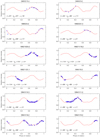 |
Fig. C.1 Observed light curves of Lacrimosa (blue points) shown with synthetic light curves corresponding to the best-fitting model with the pole direction (15°, 67°) and rotation period 14.085734 h (red curves). The viewing and illumination geometry is described by the aspect angle θ, the solar aspect angle θ0, and the solarphase angle α. |
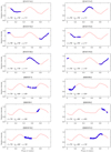 |
Fig. C.2 Observed light curves of Lacrimosa (blue points) shown with synthetic light curves corresponding to the best-fitting model with the pole direction (15°, 67°) and rotation period 14.085734 h (red curves). The viewing and illumination geometry is described by the aspect angle θ, the solar aspect angle θ0, and the solarphase angle α. |
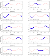 |
Fig. C.3 Observed light curves of Lacrimosa (blue points) shown with synthetic light curves corresponding to the best-fitting model with the pole direction (15°, 67°) and rotation period 14.085734 h (red curves). The viewing and illumination geometry is described by the aspect angle θ, the solar aspect angle θ0, and the solarphase angle α. |
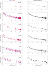 |
Fig. C.4 Left: observed sparse photometric data with their brightness reduced to a unit distance from the Sun and the Earth (blue points) and synthetic data produced by the best-fitting model with the pole direction (15°, 67°) and rotation period 14.085734 h (red points). Right: residuals (the difference between data and model) plotted on the model phase curve (dashed curve). |
References
- Bertotti, B., Farinella, P., & Vokrouhlický, D. 2003, Physics of the Solar System – Dynamics and Evolution, Space Physics and Spacetime Structure (Dordrecht: Kluwer Academic Press) [Google Scholar]
- Binzel, R. P. 1987, Icarus, 72, 135 [NASA ADS] [CrossRef] [Google Scholar]
- Breiter, S., & Michalska, H. 2008, MNRAS, 388, 927 [NASA ADS] [CrossRef] [Google Scholar]
- Breiter, S., Nesvorný, D., & Vokrouhlický, D. 2005, AJ, 130, 1267 [NASA ADS] [CrossRef] [Google Scholar]
- Colombo, G. 1966, AJ, 71, 891 [NASA ADS] [CrossRef] [Google Scholar]
- Čapek, D., & Vokrouhlický, D. 2004, Icarus, 172, 526 [NASA ADS] [CrossRef] [Google Scholar]
- Ďurech, J., Sidorin, V., & Kaasalainen, M. 2010, A&A, 513, A46 [NASA ADS] [CrossRef] [EDP Sciences] [Google Scholar]
- Ďurech, J., Kaasalainen, M., Herald, D., et al. 2011, Icarus, 214, 652 [NASA ADS] [CrossRef] [Google Scholar]
- Ďurech, J., Carry, B., Delbò, M., Kaasalainen, M., & Viikinkoski, M. 2015, in Asteroids IV, eds. P. Michel, F. E. DeMeo, & W. F. Bottke, 183 [Google Scholar]
- Ďurech, J., Delbo’, M., Carry, B., Hanuš, J., & Alí-Lagoa, V. 2017, A&A, 604, A27 [NASA ADS] [CrossRef] [EDP Sciences] [Google Scholar]
- Ďurech, J., Hanuš, J., & Vančo, R. 2019, A&A, 631, A2 [CrossRef] [EDP Sciences] [Google Scholar]
- Hanuš, J., Brož, M., Ďurech, J., et al. 2013, A&A, 559, A134 [NASA ADS] [CrossRef] [EDP Sciences] [Google Scholar]
- Hanuš, J., Ďurech, J., Oszkiewicz, D. A., et al. 2016, A&A, 586, A108 [NASA ADS] [CrossRef] [EDP Sciences] [Google Scholar]
- Haponiak, J., Breiter, S., & Vokrouhlický, D. 2020, Celest. Mech. Dyn. Astron., 132, 24 [CrossRef] [Google Scholar]
- Henrard, J. 1982, Celest. Mech., 27, 3 [NASA ADS] [CrossRef] [MathSciNet] [Google Scholar]
- Henrard, J., & Murigande, C. 1987, Celest. Mech., 40, 345 [NASA ADS] [CrossRef] [Google Scholar]
- Herald, D., Gault, D., Anderson, R., et al. 2020, MNRAS, 499, 4570 [Google Scholar]
- Hirayama, K. 1918, AJ, 31, 185 [NASA ADS] [CrossRef] [Google Scholar]
- Jehin, E., Gillon, M., Queloz, D., et al. 2011, Messenger, 145, 2 [Google Scholar]
- Kaasalainen, M., & Lamberg, L. 2006, Inverse Probl., 22, 749 [NASA ADS] [CrossRef] [Google Scholar]
- Kaasalainen, M., Torppa, J., & Muinonen, K. 2001, Icarus, 153, 37 [Google Scholar]
- Kochanek, C. S., Shappee, B. J., Stanek, K. Z., et al. 2017, PASP, 129, 104502 [Google Scholar]
- Laskar, J. 1988, A&A, 198, 341 [NASA ADS] [Google Scholar]
- Masiero, J. R., Mainzer, A. K., Grav, T., et al. 2011, ApJ, 741, 68 [NASA ADS] [CrossRef] [Google Scholar]
- Masiero, J. R., Mainzer, A. K., Bauer, J. M., et al. 2013, ApJ, 770, 7 [NASA ADS] [CrossRef] [Google Scholar]
- Nesvorný, D., & Vokrouhlický, D. 2007, AJ, 134, 1750 [NASA ADS] [CrossRef] [Google Scholar]
- Nesvorný, D., & Vokrouhlický, D. 2008, AJ, 136, 291 [NASA ADS] [CrossRef] [Google Scholar]
- Nesvorný, D., Brož, M., & Carruba, V. 2015, in Asteroids IV, eds. P. Michel, F. E. DeMeo, & W. F. Bottke, 297 [Google Scholar]
- Rubincam, D. P. 2000, Icarus, 148, 2 [NASA ADS] [CrossRef] [Google Scholar]
- Saillenfest, M., Laskar, J., & Boué, G. 2019, A&A, 623, A4 [CrossRef] [EDP Sciences] [Google Scholar]
- Shappee, B., Prieto, J., Stanek, K. Z., et al. 2014, in Amer. Astron. Soc. Meet. Abstr., 223, 236.03 [Google Scholar]
- Slivan, S. M. 2002, Nature, 419, 49 [Google Scholar]
- Slivan, S. M., & Binzel, R. P. 1996, Icarus, 124, 452 [NASA ADS] [CrossRef] [Google Scholar]
- Slivan, S. M., & Molnar, L. A. 2012, Icarus, 220, 1097 [NASA ADS] [CrossRef] [Google Scholar]
- Slivan, S. M., Binzel, R. P., Crespo da Silva, L. D., et al. 2003, Icarus, 162, 285 [NASA ADS] [CrossRef] [Google Scholar]
- Slivan, S. M., Binzel, R. P., Boroumand, S. C., et al. 2008, Icarus, 195, 226 [NASA ADS] [CrossRef] [Google Scholar]
- Slivan, S. M., Binzel, R. P., Kaasalainen, M., et al. 2009, Icarus, 200, 514 [NASA ADS] [CrossRef] [Google Scholar]
- Stephens, R. D. 2014, Minor Planet Bull., 41, 13 [Google Scholar]
- Szakáts, R., Müller, T., Alí-Lagoa, V., et al. 2020, A&A, 635, A54 [NASA ADS] [CrossRef] [EDP Sciences] [Google Scholar]
- Tonry, J. L., Denneau, L., Heinze, A. N., et al. 2018, PASP, 130, 064505 [NASA ADS] [CrossRef] [Google Scholar]
- Vokrouhlický, D., & Čapek D. 2002, Icarus, 159, 449 [NASA ADS] [CrossRef] [Google Scholar]
- Vokrouhlický, D., Nesvorný, D., & Bottke, W. F. 2003, Nature, 425, 147 [NASA ADS] [CrossRef] [PubMed] [Google Scholar]
- Vokrouhlický, D., Nesvorný, D., & Bottke, W. F. 2006, Icarus, 184, 1 [NASA ADS] [CrossRef] [Google Scholar]
- Vokrouhlický, D., Bottke, W. F., Chesley, S. R., Scheeres, D. J., & Statler, T. S. 2015, in Asteroids IV, eds. P. Michel, F. E. DeMeo, & W. F. Bottke, 509 [Google Scholar]
- Ward, W. R., & Hamilton, D. P. 2004, AJ, 128, 2501 [NASA ADS] [CrossRef] [Google Scholar]
- Warner, B. D., Harris, A. W., & Pravec, P. 2009, Icarus, 202, 134 [Google Scholar]
Lacrimosa belongs to the largest members in the Koronis family. In fact, Masiero et al. (2013) opted to call the cluster “Lacrimosa family”, which proved unsuitable because of a long tradition and history of the Koronis family since the pioneering work of Hirayama (1918).
All Tables
All Figures
|
Fig. 1 Shape model of Lacrimosa for pole direction (15°, 67°) shown from equatorial level (left and center, 90° apart) and pole-on (right). |
| In the text | |
|
Fig. 2 Projections of two occultations from December 31, 2003 (left), and October 20, 2016 (right). Individual observations are shown as straight red lines. Solid lines are photoelectric observations, dashed are visual observations, and dotted are negative observations. Timing errors are displayed as gray strips. The blue solid silhouette is that of the best-fit model, the dotted silhouette is of the second pole solution, and the dashed silhouette is of the IR-based shape model without any scaling. North is up, west to the right. |
| In the text | |
|
Fig. 3 Obliquity ε2 of the Cassini state 2 as a function of the dynamical ellipticity Δ (see Eq. (A.3)). Orbital parameters of (208) Lacrimosa are assumed. Left panel: nominal rotation period P = 14.085734 h of (208) Lacrimosa used. The solid line labeled C2(s6) provides ε2 for the s6 (forced) frequency mode of the nodal precession. The spin-orbit resonance onsets for Δ are denoted by the light-gray dashed line (transition determined by the Eq. (A.7) condition); beyond this value the Cassini state 2 becomes an equilibrium point of the spin-orbit resonance,whose maximum extension in obliquity is shown by the gray area. Solid line labeled C2 (s) provides ε2 for the s (proper) mode of the nodal precession. Here the spin-orbit resonance does not exist. Red symbols show obliquity and Δ values for a little less than 1000 solutions for (208) Lacrimosa from the bootstrap method discussed in Sect. 2 and using only the optical light-curve observations. The blue star is the nominal, best-fit solution. Right panel: same as in the left panel, but now for a hypothetical, longer rotation period of P = 28 h. Now the spin–orbit resonance exists beyond some critical Δ value for both frequencies s6 and s. |
| In the text | |
|
Fig. 4 Top panel: time evolution of the osculating obliquity ε for (208) Lacrimosa over the 2 Myr interval using numerical integration of Eq. (A.1) with Tng = 0. The initial conditions at the present epoch from the best-fit rotation state solution (P = 14.085734 h, λ = 15.2° and β = 66.9°) and Δ = 0.23. The short-period oscillations are due to the proper term of nodal precession with frequency s (which have a period of ≃2π∕(s − s6) ≃ 32 kyr). The long-period and large-amplitude oscillations of ≃745 kyr are due to libration about the resonant Cassini state 2 associated with frequency s6 (“the Slivan state”). Bottom panel: phase portrait of the Colombo top model for the s6 frequency and precession constant α ≃ 29.75 arcsec yr−1 (i.e., P = 14.085734 h and Δ = 0.23 in Eq. (A.4)); the ordinate is either cosε6 (left) or ε6 (right) and the abscissa is φ6. The light-gray curves are isolines of the first integral C(ε6, φ6) = constant given by Eq. (A.11). Critical curves of the spin-orbit resonance, namely the separatrix and the stable equilibrium C2, are highlighted in red. The black curve is the numerically integrated pole of (208) Lacrimosa from the top projected into the plane of these variables; the blue diamond is the current position of the pole. |
| In the text | |
|
Fig. 5 Top panel: time evolution of the osculating obliquity ε for (208) Lacrimosa over the 2 Myr interval using numerical integration of Eq. (A.1) with Tng = 0. The initial conditions at the present epoch from the best-fit rotation state solution (P = 14.085734 h, λ = 15.2° and β = 66.9°) and Δ = 0.35. The amplitude of the oscillations, which is larger than the proper inclination (≃ 2.15°), is forced by the Cassini state 2 of the s frequency at ≃6.5° (see Fig. 3). Bottom panel: phase portrait of the Colombo top model for the s6 frequency and precession constant α ≃ 45.27 arcsec yr−1 (i.e., P = 14.085734 h and Δ = 0.35 in Eq. (A.4)); the ordinate is either cosε6 (left) or ε6 (right) and the abscissa is φ6. The light-gray curves are isolines of the first integral C(ε6, φ6) = constant given by Eq. (A.11). Critical curves of the spin-orbit resonance, namely the separatrix and the stable equilibrium,are highlighted in red. The black curve is the numerically integrated pole of (208) Lacrimosa from the top projected into the plane of these variables; the blue diamond is the current position of the pole. |
| In the text | |
|
Fig. 6 Same as in Fig. 5, but here the bottom panel shows phase space coordinates of the Colombo top model for the s frequency. As shown in Fig. 3, the Cassini resonance does not exist and the Cassini state 2 has an obliquity of ≃ 6.5° (red point). Lacrimosa’s spin vector circulates about C2 (black line) and follows the isolines of the first integral (A.11) more closely than in Fig. 5. |
| In the text | |
|
Fig. 7 Example of a possible long-term evolution of the rotation state for (208) Lacrimosa. Rotation period P (top), osculating obliquity ε (middle-up),and longitude φ in the orbital frame associated with the s6-frequency and s-frequency term of the nodal precession (middle-down and bottom; note φ is measured from an axis 90° away from the corresponding nodal line). The gray dots are densely output osculating values (with a time-step of 5 kyr). Black symbols in the obliquity panel are average values in a 2 Myr running window; black symbols in the bottom panels are maximum and minimum values of the respective longitude in a 2 Myr running window. The dynamical model uses solar gravitational torque and the YORP effect with parameters determined from the best-fitting solution in Sect. 2. The red lines in the upper two panels show the present state of (208) Lacrimosa for reference. At the epoch of ≃ 2.4 Gyr, the propagated spin evolution roughly matches the present state (as indicated by the gray arrows). At ≃ 1.45 Gyr (verticaldashed line 1), the solution jumps over the Slivan state of the s6 precession frequency, where other large Koronis prograde-rotating asteroids are located. At ≃ 2.8 Gyr (vertical dashed line 2), the solution starts to closely follow the Cassini state 2 associated with the s precession frequency. This is allowed by (i) the low obliquity (where C2 is located), and (ii) the increasing rotation period. The Cassini resonance formally bifurcates when the rotation period reaches ≃24.4 h, i.e., at ≃4.1 Gyr. Finally, at ≃5.63 Gyr (vertical dashed line 3), the small-amplitude oscillations about the resonant Cassini state 2 in the s precession frequency frame become perturbed by an overlap with the Cassini resonance associated with the s6 precession frequency. The simulations had an initial rotation period of 12.25 h and an initial obliquity of 70°. |
| In the text | |
|
Fig. 8 Same as in Fig. 7, but now for a different initial rotation period of 9 h. In many respects, the evolution is similar to that shown in the previous figure with one important exception: at ≃ 2.25 Gyr (vertical dashed line 1) the spin state becomes captured in the Slivan state of the s6 precession frequency; it remains located in the Slivan state until ≃5 Gyr (verticaldashed line 2), when the amplitude of resonant libration grows to 180°. Consequently, the spin state leaves the Slivan state and continues to evolve primarily by YORP torques: the obliquity drifts to small values and the rotation period slowly increases; at ≃ 5.85 Gyr (highlighted by the arrows), both roughly match the current values of (208) Lacrimosa. As the rotation period continues to grow, the spin evolution follows the trend seen also in Fig. 7: it starts to closely follow the Cassini state 2 associated with the s precession frequency (eventually becoming captured in the corresponding Slivan state). |
| In the text | |
|
Fig. 9 Left panel: capture probability to the spin-orbit resonance in a Colombo top model with an adiabatically slow change in the asteroid rotation period P (at the abscissa). Heliocentric orbit of (208) Lacrimosa, dynamical ellipticity Δ = 0.35, and s6 mode of the orbital node precession were used. With these assumptions, the resonance bifurcates at ≃ 8.73 h rotation period (vertical dashed line). The red line indicates probability P+ of a capture from orbits originally circulating about the Cassini state C3, the blue line indicates probability P− of a capture from orbits originally circulating about the Cassini state C1. The analytical theory of Henrard & Murigande (1987) is briefly recalled in the appendix; see Eqs. (A.12) and (A.13). The upper abscissa shows obliquity ε2 of the Cassini state C2, the equilibrium point of the resonance. Right panel: phase portrait of the Colombo top for rotation period P = 14.085734 h (other parameters as above). The gray curves are isolines of the integral C(ε, φ) = constant given by Eq. (A.11). The black curve is the separatrix and the black dot shows the location of the Cassini state C2. The arrows schematically indicate the capture in the resonance from orbits originally circulating about the Cassini state C1 (blue) and C3 (red); in a model where only the rotation period P slowly changes, the former occurs for a decrease in P and the latter occurs for an increase in P. |
| In the text | |
|
Fig. C.1 Observed light curves of Lacrimosa (blue points) shown with synthetic light curves corresponding to the best-fitting model with the pole direction (15°, 67°) and rotation period 14.085734 h (red curves). The viewing and illumination geometry is described by the aspect angle θ, the solar aspect angle θ0, and the solarphase angle α. |
| In the text | |
|
Fig. C.2 Observed light curves of Lacrimosa (blue points) shown with synthetic light curves corresponding to the best-fitting model with the pole direction (15°, 67°) and rotation period 14.085734 h (red curves). The viewing and illumination geometry is described by the aspect angle θ, the solar aspect angle θ0, and the solarphase angle α. |
| In the text | |
|
Fig. C.3 Observed light curves of Lacrimosa (blue points) shown with synthetic light curves corresponding to the best-fitting model with the pole direction (15°, 67°) and rotation period 14.085734 h (red curves). The viewing and illumination geometry is described by the aspect angle θ, the solar aspect angle θ0, and the solarphase angle α. |
| In the text | |
|
Fig. C.4 Left: observed sparse photometric data with their brightness reduced to a unit distance from the Sun and the Earth (blue points) and synthetic data produced by the best-fitting model with the pole direction (15°, 67°) and rotation period 14.085734 h (red points). Right: residuals (the difference between data and model) plotted on the model phase curve (dashed curve). |
| In the text | |
Current usage metrics show cumulative count of Article Views (full-text article views including HTML views, PDF and ePub downloads, according to the available data) and Abstracts Views on Vision4Press platform.
Data correspond to usage on the plateform after 2015. The current usage metrics is available 48-96 hours after online publication and is updated daily on week days.
Initial download of the metrics may take a while.