| Issue |
A&A
Volume 652, August 2021
|
|
|---|---|---|
| Article Number | A37 | |
| Number of page(s) | 16 | |
| Section | Numerical methods and codes | |
| DOI | https://doi.org/10.1051/0004-6361/202140465 | |
| Published online | 06 August 2021 | |
Investigating ionospheric calibration for LOFAR 2.0 with simulated observations
1
Hamburger Sternwarte, University of Hamburg, Gojenbergsweg 112, 21029 Hamburg, Germany
e-mail: This email address is being protected from spambots. You need JavaScript enabled to view it.
2
INAF – Istituto di Radioastronomia, Via P. Gobetti 101, 40129 Bologna, Italy
Received:
1
February
2021
Accepted:
7
May
2021
Abstract
Context. There are a number of hardware upgrades for the Low-Frequency Array (LOFAR) currently under development. These upgrades are collectively referred to as the LOFAR 2.0 upgrade. The first stage of LOFAR 2.0 will introduce a distributed clock signal and allow for simultaneous observations using all the low-band and high-band antennas of the array.
Aims. Our aim is to provide a tool for obtaining accurate simulations for LOFAR 2.0.
Methods. We present our software for simulating LOFAR and LOFAR 2.0 observations, which includes realistic models for all important systematic effects such as the first- and second-order ionospheric corruptions, time-variable primary-beam attenuation, station-based delays, and bandpass response. The ionosphere is represented as a thin layer of frozen turbulence. Furthermore, thermal noise can be added to the simulation at the expected level. We simulate a full eight-hour simultaneous low- and high-band antenna observation of a calibrator source and a target field with the LOFAR 2.0 instrument. The simulated data are calibrated using readjusted LOFAR calibration strategies. We examine novel approaches of solution-transfer and joint calibration to improve direction-dependent ionospheric calibration for LOFAR.
Results. We find that the calibration of the simulated data behaves very similarly to a real observation and reproduces certain characteristic properties of LOFAR data, such as realistic solutions and image quality. We analyze strategies for direction-dependent calibration of LOFAR 2.0 and find that the ionospheric parameters can be determined most accurately when combining the information of the high-band and low-band in a joint calibration approach. In contrast, the transfer of total electron content solutions from the high-band to the low-band shows good convergence but is highly susceptible to the presence of non-ionospheric phase errors in the data.
Key words: methods: data analysis / instrumentation: interferometers / techniques: interferometric / radio continuum: general
© ESO 2021
1. Introduction
The Low-Frequency Array (LOFAR) is an interferometer working at low (< 1 GHz) and ultra-low (< 100 MHz) radio frequencies. Most of its stations are located in the Netherlands and it has been operational since 2010 (van Haarlem et al. 2013). It conducts observations in a spectral band close to the low-frequency edge of the radio window, which has received reinforced attention in the last decade. Together with other new generation instruments, such as the Murchison Widefield Array (MWA, Tingay et al. 2013) and the Long Wavelength Array (LWA, Taylor et al. 2012), LOFAR pioneers the technological ground for the ambitious plans on the Square Kilometer Array (SKA, Dewdney et al. 2009), which include the low-frequency interferometer SKA-low.
Among the most important research prospects in low-frequency radio astronomy are deep surveys, where phenomena such as the extended emission in galaxy clusters and high-redshift radio galaxies are studied. These sources oftentimes remain undetectable at higher frequencies due to their steep spectral energy distribution. Further science cases include the search for the epoch of reionization hydrogen line, cosmic magnetism, radio detection of exoplanets, mapping of the star-formation history of the universe as well as the observation of pulsars and radio transients.
A challenging limitation for the scientific value of wide-field images is imposed by the direction-dependent corruptions introduced by the ionosphere for Earthbound measurements of cosmic radio signals. This is especially problematic at ultra-low frequencies, where the impact of the ionosphere becomes increasingly dramatic. To accurately account for ionospheric effects during calibration, the development of a new generation of direction-dependent calibration strategies together with the corresponding software environment was initiated during the last decade (Tasse et al. 2021; de Gasperin et al. 2020; Albert et al. 2020; van Weeren et al. 2016). Nevertheless, excellent image fidelity is still hard to achieve with LOFAR for complex fields (e.g. towards the Galactic plane), during exceptionally active ionospheric conditions, and for the lowest part of the frequency band (≲40 MHz).
This has motivated the implementation of the LOFAR 2.0 upgrade, which is going to increase system performance, especially for the low-band antenna (LBA) part of the array (Hessels et al., in prep.). This upgrade will allow for simultaneous observations with the low-band and high-band antennas (HBA), and thus enable novel calibration algorithms that combine information from both antennas.
To make efficient use of the upgraded hardware, it is important to examine new calibration strategies for LOFAR 2.0 prior to the deployment of the upgraded hardware. We developed the LOFAR Simulation Tool (LoSiTo) to simulate a full 8 h simultaneous calibrator and target field observations with the upgraded LOFAR 2.0 system. First, we calibrated the simulated data for instrumental and direction-independent effects, relying mostly on standard LOFAR tools. Then, we investigated novel approaches for direction-dependent calibration with the aim of improving the ionospheric calibration of the LBA system.
This paper is arranged as follows. In Sect. 2, we discuss the current limitations of LOFAR and the improvements that will be introduced by LOFAR 2.0. In Sect. 3, we present models for the instrumental and ionospheric systematic errors in LOFAR 2.0 observations and estimate the noise level of the upgraded array. The implementation of these models in a simulation software as well as the setup of the simulated observation is described in Sect. 4. Next, in Sect. 5, we proceed with the calibration of the simulated data and investigate how the direction-dependent calibration for LBA could be improved by solution-transfer or joint calibration.
2. LOFAR and future upgrades
LOFAR is an array consisting of 55 stations spread across Europe. Three different station types with different hardware configurations exist: the central part of the array is composed of 24 core stations (CS); these are spread across an area in the northeast of the Netherlands that is less than 4 km wide. Another 16 stations are also located in the Netherlands, further away from the core, they are called remote stations (RS). The international part of the array consists of 15 more stations in eight European countries. Each LOFAR station hosts a field of dipoles operating as a phased array, with two drastically different dipole designs that are employed. The LBA are sensitive in the frequency range of 10 MHz−90 MHz. Additionally, the upper part of the frequency bandwidth of LOFAR is covered by the HBA, which are sensitive to the range from 110 MHz to 240 MHz. Each Dutch station is equipped with 96 LBA dipoles and 2 × 24 (CS) respectively 48 (RS) HBA tiles. The antenna signals are locally digitized in receiver units (RCUs), there are a total of 48 RCUs per Dutch station. Hence, operation is limited to either all 48 HBA tiles or 48 out of the 96 LBA dipoles (van Haarlem et al. 2013). Consequently, with regard to LBA, not all the existing dipoles are utilized and the potential sensitivity has not been reached.
Currently, the clock signals for all remote and international stations are provided by GPS-synchronized rubidium clocks. These clocks show the presence of a 𝒪(10 ns h−1) clock drift which causes non-negligible phase errors in the data (de Gasperin et al. 2019; van Weeren et al. 2016).
The LOFAR 2.0 upgrade is designed to overcome these limitations and consists of multiple projects (Hessels et al., in prep.). In this work, we focus on the changes introduced by the Digital Upgrade for Premier LOFAR Low-band Observing (DUPLLO). DUPLLO is a funded project (Dutch Research Council (NWO) 2018), with its main focus based on improving the performance of the LBA system. Among the key components of DUPLLO is the deployment of improved station electronics. The number of RCUs per station will be tripled, this is going to allow for simultaneous observations with all 96 LBA dipoles as well as the 48 HBA tiles. The consequences of this move will be an increase of sensitivity and field of view (FoV) in LBA observations and the possibility of innovative calibration algorithms that can exploit the simultaneous observations to derive more accurate direction-dependent calibration solutions. The second improvement introduced by DUPLLO will be a new clock system. A “White Rabbit” ethernet-based timing distribution system (Lipiński et al. 2011) will be employed to synchronize all Dutch stations with a single clock (van Cappellen 2019). The roll-out of the first stage of LOFAR 2.0, which includes DUPLLO, is anticipated for April 2022 and full operation is expected for December 2023 (van Cappellen 2019).
3. Model corruptions
To accurately simulate LOFAR observations, realistic models for the corrupting effects present in the observations are required. Systematic effects related to physical and instrumental phenomena may be extracted from calibration solutions due to their characteristic properties and dependencies. In de Gasperin et al. (2019), measurements of the bright calibrator source 3C196 were analyzed and all major corrupting effects present in LOFAR observations could be isolated from the calibration solutions. We take these effects as a reference for the systematics that need to be included in realistic simulations. A summary of these effects together with the dominant noise components is presented in Table 1.
Systematic effects and noise components in LOFAR observations.
The mathematical framework of radio-interferometry is given by the radio interferometer measurement equation (hereinafter RIME; see Hamaker et al. 1996; Smirnov 2011). The RIME connects the complex visibility V, which is the quantity measured at the interferometer, to the sky brightness distribution B. Systematic effects enter the RIME as Jones-matrices Ja. Jones matrices are 2 × 2 matrices defined on the linear (or equivalently, circular) polarization basis of the electromagnetic field. If multiple effects are present, the total Jones matrix is the matrix product of the individual matrices. The order for matrix-multiplication is given by the order in which the effects occur along the signal path: Jtotal = J1 ⋅ … ⋅ Jn. The shape of the Jones-matrix is determined by the polarization-dependence of the underlying effect. A full formulation of the RIME is given by:
 (1)
(1)
where l, m and  are the components of the source direction unit vector and u, v, w are the components of the baseline vector measured in wavelengths.
3.1. Ionosphere model
The ionized plasma of the upper atmosphere interferes with radioastronomic observations in a variety of ways. Series expansion of the diffractive index n(ν) in ν−1 allows us to describe this interference by a few simple effects (Datta-Barua et al. 2008). The dominant ionospheric effect is a dispersive delay which expresses itself as a scalar phase error Δϕ with a characteristic frequency dependence of ∝ν−1 (Mevius et al. 2016):
![Mathematical equation: $$ \begin{aligned} \Delta \phi = -84.48 \left[\frac{{\mathrm{d} }\mathrm{TEC}}{1\,\mathrm{TECU}}\right]\left[\frac{100\,\mathrm{MHz}}{\nu }\right]\,\mathrm{rad}. \end{aligned} $$](/articles/aa/full_html/2021/08/aa40465-21/aa40465-21-eq3.gif) (2)
(2)
This phase error depends on the line of sight integrated electron density Ne, which is referred to as the total electron content (TEC):
 (3)
(3)
The TEC is most commonly measured in total electron content units (TECU, 1 TECU = 10 × 1016 m−2). Since the RIME is insensitive to a global scalar phase, only the differential TEC between the stations is relevant for the dispersive delay.
Another ionospheric effect that is non-negligible at the frequency range of LOFAR is Faraday rotation. This effect is of second order in ν−1 and hence, especially problematic at the lowest frequencies. It manifests itself as rotation in the plane of linear polarization. The line-of-sight contribution to the Faraday rotation depends on the magnetic field B and the free electron density and can be summarized into the rotation measure (RM):
 (4)
(4)
Here, e is the electron charge, me the electron mass, c the speed of light in vacuum, ϵ0 the vacuum permittivity, and θ the angle between the magnetic field vector and the line-of-sight. The corresponding rotation angle β is given by:
 (5)
(5)
Ionospheric rotation does also affect unpolarized signals: the magnetic flux density and the free electron number density vary between signal paths. This introduces a relative rotation angle between different stations and source directions. This effect is known as differential Faraday rotation and can, on the basis of linear polarization, be described by a rotational Jones matrix. This differential rotation causes amplitude and phase errors and may de-correlate the signal in extreme cases. The impact of this effect becomes important for frequencies below 80 MHz and baselines longer than 10 km (Mevius 2018a).
The next important higher order effect is of third order in ν−1 and manifests as dispersive delay, similar to the first order effect. In de Gasperin et al. (2018), it was found that this effect is only important for frequencies below 40 MHz. Since the effect is negligible for most of the frequency range observed by LOFAR and also quadratic in the free electron density and hence, harder to model compared to the first and second order effects, we have chosen to not include it in the simulation.
To obtain a realistic model of the ionosphere, a number of characteristic properties have to be considered. The scale and structure of the electron content must be in reasonable agreement with reality. Furthermore, the electron distribution must be spatially and temporally coherent. We employ the thin-layer model to describe the free electron density of the ionosphere. It represents the ionosphere as two-dimensional spherical shell at a height of hion around the Earth. This approximation is motivated by the vertical structure of the ionosphere. The majority of the free electrons are constrained within the ionospheric F-layer between 200 km and 450 km. Contracting the three-dimensional structure onto a two-dimensional sphere drastically reduces the complexity of the model while maintaining many of the important characteristics, such as spatial coherency and to some accuracy, the elevation dependence of the projected electron content (see Martin et al. 2016).
In the thin-layer approximation, the ionosphere is fully parameterized by a two-dimensional distribution of the vertical total electron content (vTEC). This distribution is hereinafter referred to as a TEC-screen. The TEC value corresponding to a specific signal path is evaluated at the ionospheric pierce point, which is defined as the point where the source direction vector pierces the TEC-screen.
For sources which are not directly at the zenith, an air-mass factor has to be taken into account to derive the slant TEC (sTEC) along the line of sight. Projection leads to an increase of the TEC for directions further away from the zenith:
 (6)
(6)
where θion is the pierce angle. Since we model the Earth as a sphere of radius RE, the pierce angle can be calculated from the source elevation θ′ according to the law of sines (Martin et al. 2016):
 (7)
(7)
which allows us to derive the corresponding sTEC for any direction:
 (8)
(8)
A substantial fraction of ionospheric inhomogeneity can be attributed to turbulent phenomena (Materassi et al. 2019; Giannattasio et al. 2018). Ionospheric turbulence can be approximately described by a process where energy is injected into a system with high Reynolds number at large spacial scales and iteratively distributed to smaller scales (Thompson et al. 2017). This self-similarity leads to a refractive-index power spectrum Φ(k) that follows a power-law shape:
 (9)
(9)
where k is the spatial frequency. In case of pure Kolmogorov turbulence, the spectral index β = 11/3 (Tatarski 1961, 1971). Taking the finite outer scale L0 of the turbulence into consideration yields:
 (10)
(10)
which in the β = 11/3 case describes the von Kármán spectrum (von Karman 1948).
Previous studies with LOFAR have confirmed the power-law shape, but found a slightly steeper spectrum of β = 3.89 ± 0.01 (Mevius et al. 2016; de Gasperin et al. 2019)1. We adopt this empirically derived value for our ionospheric model.
To generate a turbulent screen in LoSiTo, the algorithm described in Buscher (2016) is employed. This algorithm follows an approach based on the fast Fourier transform method and treats large and small spatial frequencies separately to increase computational performance. Furthermore, it makes use of the frozen turbulence approximation. In this approximation, the change of the turbulent structure is assumed to be negligible with respect to the bulk velocity of the ionosphere. Therefore, the ionosphere is modeled as a static grid moving across the LOFAR stations. To optimize performance, the extent of the screen is constrained to the outermost pierce-points for each time-step. We scale the dTEC sampled from the TEC-screen such that the maximum dTEC across all stations, directions, and times is 0.25 TECU. We add a homogeneous component of the TEC at 7.0 TECU. The daily ionospheric variation is included using a simple sinusoidal pattern: The total electron content peaks at 3:00 pm and drops to a level of 10% at 3:00 am.
We place our model-ionosphere at a height of hion = 250 km, around the typical location of the peak electron density at the latitude of LOFAR as modeled by the international reference ionosphere (Bilitza 2018). The ionospheric grid is simulated at an angular resolution of 1 arcmin (≈72 m) and moves from West to East at a velocity of 20 m s−1.
One snapshot of such a TEC-screen is shown in Fig. 1. We show the pierce-points of five selected LOFAR stations. It is apparent that all the CS observe a similar ionosphere, the dTEC between different directions dominates compared to the dTEC between different CS. The most distant RS observe a different part of the ionosphere.
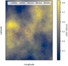 |
Fig. 1. Snapshot of a simulated turbulent TEC-screen with the parameters β = 3.89 and hiono = 250 km. Each circle marks one pierce-point, circles of the same color show pierce-points for different directions belonging to the same station. Only pierce-points belonging to one of the centermost stations (CS001), the most distant central station (CS501) as well as the three outermost remote stations (RS210, RS310, RS509) are displayed. |
For each pierce-point and at every time-step, the vTEC-values of the closest grid points are linearly interpolated and converted to sTEC according to Eq. (8). These values are stored in the h5parm format introduced in de Gasperin et al. (2019).
To derive the Faraday rotation from the ionospheric model, we apply the thin-layer approximation to Eq. (4):
 (11)
(11)
For the calculation of the RM, the magnetic field vector B projected onto the source-direction  and evaluated at the pierce-point is required. As magnetic field model, the implementation of the World Magnetic Model (Chulliat et al. 2015) in the RMExtract library (Mevius 2018b) is employed.
The FARADAY-operation in LoSiTo derives the RM from this magnetic model and the sTEC values stored in the h5parm file. The RM values are added to the h5parm-file in a new table. The simulated dTEC and dRM-values for three stations and three directions are displayed in Fig. 2. As expected from Eq. (11), the dTEC and dRM values are highly correlated. From our experience, the ionospheric conditions of this simulation are representative for low solar activity.
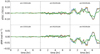 |
Fig. 2. Simulated dTEC (top panels) and dRM (bottom panels) for three stations for a source in the phase center (orange) and for sources separated from the phase center by 1.75° (blue) and 4.51° (green). The stations are at distances of 1.7 km (CS501), 6.3 km (RS205) and 55.7 km (RS509) to CS001. The values of each direction are referenced with respect to the same direction in CS001LBA. |
3.2. Primary beam
The primary beam characterizes the directional sensitivity for the interferometer components, in the case of LOFAR for the individual stations. Since LOFAR does not simply consist of single dish antennas, but follows a phased array design, the treatment of the primary beam is more complex compared to classical interferometers. For LOFAR, the primary beam can be split into two components, the element beam and the array-factor. The element beam characterizes the directional sensitivity of a single antenna element. An LBA element consist of one dipole pair, while for HBA, tiles of 16 pairs are grouped together to form one element (van Haarlem et al. 2013). The element beam varies only slowly across the sky and in time. The element beam is always pointed towards the local horizon, leading to a decline of sensitivity for low elevations. In contrast, the array-factor is a Jones-scalar, which describes the influence of the beam-forming (that is, the superposition of the element signals) on the directional sensitivity. The array factor determines the size of the instrument FoV. LoSiTo uses the LOFARBeam2 library to include both the element beam and the array factor in the simulations. This library uses results of electromagnetic simulations of the dipoles to calculate the primary beam Jones-matrices (Hamaker 2011).
Since the LOFAR 2.0 LBA system will utilize 96 dipoles per station instead of just 48, the shape of the array-factor will change. In Fig. 3, we show a comparison of the array-factor amplitude between a current LBA station, a LOFAR 2.0 LBA station, and an HBA station. We note that the LOFAR 2.0 upgrade will not just increase the size of the FoV, but also significantly reduce the side-lobe structure. The size of the primary beam at 54 MHz (full-width at half-maximum) will increase to 5.6° from 4.3° in LBA_outer. For comparison, the HBA beam in mode Dual_inner at 144 MHz is 4.8° wide.
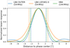 |
Fig. 3. Normalized LOFARBeam beam response (y-axis) as a function of phase center separation (x-axis) for the current 48 dipole LBA system in mode outer, the 96 dipole LOFAR 2.0 LBA system and the HBA system. The dashed vertical lines mark the primary beam FWHM of the respective system. |
3.3. Bandpass response
The bandpass describes the frequency dependence of the system’s amplitude response. Therefore, it is constant in time and does not affect the phases. It is an instrumental effect which is largely shaped by the dipole response. In reality, variations in the dipole shapes and electronics cause deviations of the bandpass between the different stations and polarizations and might also introduce a slow time-variation. This variation may be caused by changes in environmental conditions that affect dipole properties, such as humidity. The bandpass can be described by a station dependent, real diagonal matrix.
LoSiTo includes a straightforward model for the bandpass, using the average bandpass that was determined in an empirical study of the instrument in van Haarlem et al. (2013). The model for both antenna types is shown in Fig. 4. LOFAR features three HBA bandpass modes with different spectral windows. We will only consider the mode HBA-low, since in practice, this mode is used almost exclusively. While the HBA dipole response is rather flat, the response of the LBA dipoles features a prominent peak at 58 MHz with a full width at half maximum (FWHM) of 15 MHz, causing a sharp decline of sensitivity below and above the peak frequency.
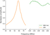 |
Fig. 4. Normalized bandpass amplitudes (y-axis) for the LBA and the most common HBA bandpass setup HBA-low as a function of frequency (x-axis). The values are adopted from an empirical study of the instrument in van Haarlem et al. (2013). |
3.4. Station based delays
An omnipresent systematic effect in radio interferometry is given by offsets in the signal timing between the interferometer stations or antennas. This is, for instance, caused by asynchronous clocks and improper calibration of electronics. Especially for long baseline instruments, the issue of accurate clock calibration across large physical distances arises.
A time delay Δt between two baseline elements introduces a phase-offset of Δϕ in the RIME:
 (12)
(12)
While this phase error follows a linear frequency dependence and is therefore a greater issue at higher frequencies, it is still non-negligible in present-day LOFAR observations. Currently, the remote and international stations receive a time signal from GPS-synchronized rubidium clocks (van Haarlem et al. 2013). The signal of these clocks drifts slowly in time, causing a 𝒪(10 ns) clock error with smooth temporal behavior. This translates to a phase-error in the order of 2π at 100 MHz. The LOFAR 2.0 upgrade will introduce a new system for the time synchronization, utilizing a distributed signal from a single clock for all Dutch stations. The requirements for the distributed single-clock signal are as follows (Bassa 2020, priv. comm.). First, the timing reference signal at Core Stations shall have a clock error of Δtrms < 0.20 ns over a one-hour period. Second, the timing reference signal at Core and Remote Stations shall have a clock error of Δtrms < 0.35 ns over an eight-hour period. We use a simple model consisting of a sinusoidal variation on top of a constant offset to include the clock drift in the simulation:
 (13)
(13)
The drift amplitude tamp, drift frequency ωclock and the clock offset toffset are drawn from Gaussian distributions independently for each station. The widths σoffset and σamplitude are determined such that the root-mean-square (rms) error of the clock signal is one third of the maximum allowed rms in the system requirements. Furthermore, the total standard deviation should be caused in equal parts by the constant offset and the sine function. The corresponding parameters are displayed in Table 2.
Numeric values for the widths of the Gaussian distributions used to construct the LOFAR 2.0 clock model.
The resulting clock offset from this model is shown in Fig. 5 for three selected stations. The corruptions are shared between the LBA and HBA parts of each station.
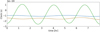 |
Fig. 5. Simulated clock delay for CS501 (blue), RS205 (orange), and RS210 (green), referenced to the clock of CS001. |
In addition to the station dependent clock delay, LOFAR data shows the presence of a nanosecond-scale time delay between the X and Y polarization of the station output. This delay, referred to as polarization misalignment, is constant in time and attributed to an inaccurate station-calibration (de Gasperin et al. 2019). We assume that this effect will be present at a similar magnitude in LOFAR 2.0. To replicate this effect, a random time offset between the polarizations is drawn from a Gaussian distribution with a width of 1 ns for each station. We sampled this effect independently for the LBA and HBA parts of a station.
3.5. Thermal noise
The achievable sensitivity of a perfectly calibrated radio interferometer is limited by the presence of noise. There are two primary noise sources: instrumental noise, for example, from the receiver and amplifier system; and sky noise, which is of cosmic origin. While for radio observations at mid and high frequencies, the instrumental component is by far dominant, this changes in the low-frequency regime, were the sky noise becomes increasingly important.
The sky noise has an ultra-steep spectrum. Assuming a power-law shape Isky ∝ ν−α, the study in Guzmán et al. (2011) found a spectral index of α = 2.57 between 45 MHz and 408 MHz. This spectral index varies across the sky, increasing strongly towards the Galactic plane. Towards the Galactic center, the brightness of the sky noise is a factor of ≈10 higher compared to the Galactic poles. For LOFAR, the sky noise is, in fact, the dominant source of noise below 65 MHz (van Haarlem et al. 2013).
The noise of a radio astronomical instrument can be expressed in terms of system equivalent flux density (SEFD). The SEFD is the flux density of a hypothetical source which induces a power in the system that is equal to the power induced by the noise. It can be calculated from the system temperature Tsys, the antenna efficiency η and the effective collection area Aeff:
 (14)
(14)
An empirical study in van Haarlem et al. (2013) determined the SEFD for the LOFAR LBA and HBA. For the LBA system, the SEFD was measured independently for the two observation modes Inner and Outer, where only the 48 inner- or outermost of the 96 dipoles are used. To estimate the SEFD for the LOFAR 2.0 LBA, we take the mean of the two modes as reference. Additionally, we scale this mean value to account for the double dipole number. The anti-proportionality to the effective collection area in Eq. (14) suggests that a doubling of the dipoles reduces the SEFD by a factor of 2. However, we adopt a more conservative scaling factor of  for two reasons: First, overlap in the effective areas of the dipoles leads to a decrease in the total area. Second, we compare the SEFD of the different HBA station types displayed in Fig. 6. The HBA arrays in the CS host 24 tiles, while the RS host 48 tiles, so they can give an idea on how a doubling of the dipoles affects the SEFD. The average SEFD of the 48 tile stations is lower by a factor of 0.75. Due to the different station layouts, this ratio cannot be transferred to LBA directly. Nevertheless, this comparison motivates our slightly more conservative value of 0.71. Our estimate for the LOFAR 2.0 LBA SEFD as well as the values adopted from van Haarlem et al. (2013) are displayed in Fig. 6.
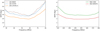 |
Fig. 6. Frequency dependence of the SEFD for different configurations of the LBA (left) and two differently equipped HBA station types (right). The estimate for the LOFAR 2.0 LBA SEFD is derived from the mean of the modes Inner and Outer. |
The noise in visibility space follows a Gaussian distribution with a frequency dependent standard deviation. This standard deviation for a frequency channel of bandwidth Δν can be computed from the SEFD of the two stations which form the baseline, the total system efficiency ηsys and the exposure τ (Taylor et al. 1999):
 (15)
(15)
We assume a system efficiency of ηsys = 0.95. Using these standard deviations, the simulated complex visibilities are corrupted with independent Gaussian noise in real and imaginary part for each frequency channel, baseline, time, and polarization.
4. LOFAR 2.0 simulation
4.1. Simulation software
We implemented the models for the corrupting effects presented in Sect. 3 in a code called the LOFAR simulation tool (LoSiTo)3. This software is a command-line program written in the Python programming language and build on top of existing LOFAR software. In the following, we provide a brief overview of the program. The main configuration file is the parameter set for which the user specifies the corrupting effects that should be included in the simulation and at which scale. Two more input files are required: one is the input sky model, where properties of the sources such as position, flux density, angular extension, spectral shape, and polarization properties are set. Such a sky model may be obtained from a source catalog or a radio image. Alternatively, it can be randomly generated using a script in LoSiTo. As last input for the simulation, a measurement set file (Schoenmaker & Renting 2011) is required. This file is the template for the simulated visibilities; furthermore, it stores the metadata of the observation, such as the observation time, frequency bands as well as location and status of the LOFAR stations. A LoSiTo simulation is composed of individual operations, each model corruption of Sect. 3 is implemented as one such operation. The simulated corruptions are stored in the h5parm data format. The central part of a simulation is the prediction. In this step, the visibilities corresponding to each source (or each patch of sources) are calculated in a Fourier-transformation from image-space to visibility-space. The Jones-matrices of the direction-dependent effects (DDE), such as the ionospheric effects and the primary beam, are calculated from the h5parm file content and multiplied with the predicted visibility matrices for the source(s). The resulting DDE corrupted visibilites for all directions are added. The Jones-matrices of the direction-independent effects (DIE) are multiplied with the visibility matrices afterwards to save computation time. This is possible because the DDE are prior to the DIE on the signal path. Lastly, noise is added to the visibilities and they are multiplied by the average bandpass response. The final product of the simulation is a measurement set file which obeys the same format as a real LOFAR observation, and thus, can be further processed with the same software. LoSiTo makes use of the software DPPP for the prediction and the application of the corruptions stored in h5parm files (van Diepen et al. 2018). The diagram in Fig. 7 presents a visualization of the architecture of LoSiTo.
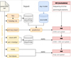 |
Fig. 7. Diagram of LoSiTo. As input, a parameter set, a sky model, and a template measurement set are required. Orange boxes represent DDE, while yellow boxes represent DIE. |
4.2. Full simulation setup
We simulate a full eight-hour LOFAR 2.0 observation of a calibrator source and a target field using the Dutch LBA and HBA stations simultaneously. For the LBA system, multi-beam observing allows to point in parallel at both target and the calibrator during the whole observation. This is not possible for HBA, were we simulate a short calibrator scan of ten minutes at the beginning of the observation. The setup of the simulated observation is shown in Table 3. Since target and calibrator field are usually located at large angular separation, they were simulated using independent ionospheric models. The station-dependent instrumental effects of bandpass, clock, and polarization alignment are shared between the calibrator and target data set.
Setup of the simulated observation.
We extracted the sky model for the target from a real LOFAR LBA observation of the field around the galaxy cluster Abell 1033 using the software PyBDSF (Mohan & Rafferty 2015). We corrected the sky model for the primary beam attenuation and set the spectral shape of all sources to a power law with a typical radio-spectral index of 0.8 (Mahony et al. 2016). We manually adjusted the flux density of the bright, resolved source in the center of the field to make it less dominant. Furthermore, we discarded all sources fainter than 0.2 Jy to decrease computational cost. Lastly, to further improve computational efficiency, we grouped sources in close proximity into patches. The DDE are not applied to each individual source but to each patch of sources, taking the flux-weighted centroid of the source locations as reference. Further away than 2.5° from the phase center, sources are grouped into larger patches. The resulting sky model is displayed in Fig. 8, it contains 340 sources in 59 patches, the total flux density is 225.8 Jy at 54 MHz.
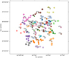 |
Fig. 8. Input sky model of the simulation. The model is extracted from a real LOFAR observation of the target field. It contains 340 sources grouped into 59 patches, the total flux density is 226 Jy at 56 MHz. Circles correspond to source locations. Sources are color-coded according to their patch membership, patch centers are marked by an “X” and labeled. |
For the calibrator observation, we use an existing model of the standard LOFAR calibrator source 3C196 which has a total flux density of 138.8 Jy at 54 MHz. We create the input measurement sets using a script available in LoSiTo. This way, we receive measurement sets for LBA and HBA with identical time-steps and pointing information. To take into account the changes introduces in the LOFAR 2.0 upgrade, we set all 96 LBA dipoles for each station to active.
We ran the simulation including all the corruptions discussed in Sect. 3. The full computation time for the simulation was 53 h using eight compute nodes equipped with Intel Xeon E5-1650 six-core processors. The primary bottleneck in terms of computation time is the prediction which depends on the number of patches and sources present in the sky model. The simulated data have been made publicly available4.
5. Calibration
Simultaneous LBA and HBA observations will offer new prospects for ionospheric calibration. Since the same region of the ionosphere will be observed in both parts of the array, the underlying parameters describing the ionospheric corruption in the data are identical. Consequently, combining the information of the low- and high-band observations could allow us to determine the ionospheric parameters more accurately and hence, derive more exact calibration solutions. This strategy is possible since both dipole systems have a comparable primary beam size which allows us to observe a sufficient number of calibrator sources in both parts of the array. It could especially benefit the LBA where the calibration of DDE is made more difficult due to the increased noise level and severity of ionospheric errors.
Currently, calibration of DDE for LOFAR mostly follows a brute-force attempt: it is solved for effective Jones matrices which are assumed to be constant for small domains of time and frequency (Tasse et al. 2021; de Gasperin et al. 2020). However, to exploit the simultaneous observation, we must obtain parameters describing the underlying physical effects, such as TEC and RM, since only these values are frequency-independent and can be meaningfully translated between LBA and HBA. This drastically reduces the number of free parameters during calibration compared to the effective-Jones approach, but requires a sufficient S/N and data that is clean of other systematic errors to converge towards the correct solutions.
We focus on two approaches to exploit the simultaneous observation for calibration of the direction-dependent dTEC. One approach is the application of ionospheric solutions found in HBA to the LBA data, we will refer to this method as “solution transfer”. This idea is based on the assumption that it is easier to converge towards correct calibration solutions in HBA, since there is significantly less noise compared to LBA (see Fig. 6). However, while the HBA stations are less affected by noise, they also observe a smaller fractional bandwidth (≈0.33) compared to LBA (≈0.89) which could make it harder to fit the ν−1 spectral dependency (see Eq. (2)) of the dispersive delay. Therefore, it is not fully clear how much more accurate TEC-extraction is in HBA. In addition, we emphasize that, when applying HBA-derived solutions to LBA, it is crucial to minimize the presence of jumps in dTEC solutions. These jumps are a consequence of the local minima present in the χ2 cost function which may be almost as deep as the global minimum, depending on the bandwidth (van Weeren et al. 2016). In the case of HBA, the jumps to a local minimum might still provide accurate calibration for a significant part of the HBA bandwidth, they cause substantially stronger phase-errors when transferred to LBA since the location of the local minima shifts with frequency.
The second method of exploiting the simultaneous observations that we consider in our analysis is joint calibration. In this scenario, it is solved for dTEC using data from both LBA and HBA together to leverage the large bandwidth observed by LOFAR and improve the S/N. This approach contains more information on a larger domain and thus, carries a greater potential for calibration, at the cost of a more complex algorithm, however.
The data reduction of the simulated observation is split into three parts, if not stated otherwise, data reduction steps are carried out independently for the LBA and HBA observations. First, the instrumental systematics are derived from the calibrator observation using the strategy described in de Gasperin et al. (2019). The second step is the calibration of DIE employing an adjusted version of the pipeline presented in de Gasperin et al. (2020). The final step is the direction-dependent calibration; here, we compare the LOFAR 2.0-specific calibration strategies to the independent calibration of the LBA system.
5.1. Calibrator data reduction
To find the solutions for the calibrator observation, we assume that the model of the calibrator source is fully accurate and calibrate against the same model we used as simulation input. First, solving against this model, the polarization alignment was derived by fitting a diagonal and a rotational matrix. The phase solutions from the diagonal matrix were averaged in time to extract the relative delay between the polarizations for each station. We corrected the data for these delays. Next, the LOFAR beam model was applied and a second diagonal and rotational fit was performed to extract the Faraday rotation solutions. The Faraday rotation solutions are applied to the data. Subsequently, a diagonal Jones-matrix was fitted and the resulting amplitude solutions were averaged in time to derive the bandpass responses. From here, the calibrator pipeline in de Gasperin et al. (2019) performs additional solution steps to derive the time-dependent clock delay from phase solutions. In a procedure called clock-TEC-separation, a clock term proportional to ν and a TEC term proportional to ν−1 are fitted to the phase solutions simultaneously to separate the effects by their characteristic frequency dependence (van Weeren et al. 2016). For HBA, calibrator observations are usually not simultaneous to the target observation due to limitations imposed by the tile beam. Therefore, we skip this step for the HBA data set. For LBA, additional smoothing was required to account for the significantly smaller clock error of our LOFAR 2.0 clock model. A benefit of testing the data reduction strategy on simulated data is that we can quantify the accuracy of the calibration solutions: for LBA, the frequency-averaged relative rms error of the bandpass solutions is 1.8% and the rms error of the polarization alignment and clock delay is 7.7 ps respectively 37 ps. For HBA, the frequency-averaged relative rms error of the bandpass solutions derived from the ten minute calibrator observation is 0.3% and the rms error of the polarization alignment delays is 1.9 ps. The bandpass, polarization alignment and clock solutions were transferred to the target data and the primary beam in direction of the phase center was applied. We exploit the simultaneity of the LOFAR 2.0 observations and transfer the LBA clock solutions to the HBA observation.
5.2. Direction-independent calibration
Next, we calibrated the target field data sets, starting with direction-independent self-calibration based on the procedure described in de Gasperin et al. (2020). The aim of this is to correct for the average ionospheric effects per station and to derive a robust source model for further direction-dependent calibration. For real observations, a catalog model of the target field is used as initial model for self-calibration. To replicate this incomplete first model, we use a sparse, corrupted version of the simulation input sky model. This model was obtained by selecting only the sources within the primary beam FWHM which are brighter than 0.5 Jy at 54 MHz. Flux density errors at a standard deviation of 10% were introduced to the remaining sources, which were 70 for LBA respectively 39 for HBA.
First, we find solutions for the differential Faraday rotation: we transform the data to circular polarization basis and consider only the phase differences of the XX and YY correlations. This eliminates all contributions of scalar phase errors such as the TEC or clock drift given that for unpolarized sources, they are equally present in both diagonal entries and cancel out. We fit these circular phase differences to a model with a phase of ϕ = 0, extract the RM from the phase solutions and apply it to the data. Next, the pipeline solves for the direction-averaged dTEC in two sub-steps: first, only for the CS and the inner RS, these solutions are then applied to the data. Second, only for the outer RS, constraining all other stations to the same value. This improves the S/N when determining the large TEC-variations of the most distant stations. The solver estimates the dTEC by fitting the 1/ν term of the dispersive delay phase error. In Fig. 9, the direction-independent dTEC and RM solutions for four LBA stations are displayed on top of the corresponding input corruptions. The direction-independent solutions trace a weighted average of the input corruptions towards the different directions. For the most distant stations, the solver sometimes converged towards neighboring minima due to the presence of noise. The RM solutions are less noisy since we chose a significantly longer solution interval of 8 min instead of 4 s, however, for a few stations (such as RS509), they sometimes show a systematic deviation from the input corruptions.
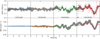 |
Fig. 9. Direction-independent ionospheric solutions towards the target field for four LBA stations. Top panels: dTEC, the bottom panels dRM. The gray curves in the background show the input corruptions towards the 59 patches. The calibration solutions are referenced to station CS001LBA and the input corruptions are referenced to the phase center direction of CS001LBA. Triangles mark solutions outside of the graph’s scale. We note that the missing variation of the input-RM for CS001 is caused by a referencing error present in the data. Simulated RM values were referenced for each direction individually instead of referencing to a single direction. However, we do not expect this to affect our analysis. |
The HBA dTEC solutions are shown in Fig. 10; due to the lower noise level, they have significantly fewer jumps. The corrected data are imaged using the WSCLEAN multi-scale algorithm (Offringa et al. 2014; Offringa & Smirnov 2017). The CLEAN-components found during imaging are used as improved model for direction-dependent calibration.
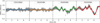 |
Fig. 10. Direction-independent TEC solutions for four HBA stations. The gray curves in the background show the input corruptions towards the 59 patches. The calibration solutions are referenced to station CS001HBA0. The input corruptions are referenced to the phase center direction of CS001HBA0. |
For LBA, the image is displayed in Fig. 11, the rms background noise is 2.0 mJy beam at a resolution of 42″ × 30″, for HBA, the noise level is 200 mJy beam at a resolution of 18″ × 14″. For comparison, typical values for the rms background noise of real LOFAR observations are around 5 mJy beam for LBA (de Gasperin et al. 2021), respectively, 380 mJy beam for HBA (Shimwell et al. 2017). The lower noise can be attributed to the improved sensitivity of LOFAR 2.0 for LBA and a reduced source density of our simulated sky model compared to a fully realistic source distribution.
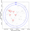 |
Fig. 11. LBA wide-field image after DIE calibration. The rms background noise is ≈2.0 mJy beam−1 at a resolution of 42″ × 30″. The DDE calibrator directions are highlighted in red, the blue dashed circles show the primary beam FWHM of the LOFAR 2.0 LBA at 54 MHz and the HBA at 144 MHz. The background color scale shows the logarithmic surface brightness in arbitrary units. |
One point that must be accounted for in LOFAR 2.0 calibration is the difference in the FoV of the low- and high band (see Fig. 11). The LBA beam at the center of the frequency band covers a 36% larger area compared to HBA. This discrepancy could be compensated for by using multiple simultaneous HBA pointings to cover one LBA pointing. Alternatively, the greater sensitivity of the HBA could justify to use regions outside of the FWHM for simultaneous calibration.
5.3. Direction-dependent calibration
The last data-reduction step is the calibration for DDE which is necessary to correct for TEC-variation across the FoV. We identify DDE-calibrators from the DIE calibrated LBA image, using the source finder PyBDSF to isolate islands of emission. We employ a grouping algorithm to merge sources in close proximity. To avoid faint and very extended sources, we place a threshold on the flux density to source area ratio and discard all sources fainter than 0.8 Jy at 60 MHz. This procedure resulted in six calibrator directions with apparent flux densities of 0.9 to 2.8 Jy, the locations of which are shown in Fig. 11. We note that for sufficient calibration of the full FoV, more calibrator directions are necessary, depending on the ionospheric conditions. However, our sample contains point-like, multi-component and complex sources, and can thus give a good indication of the convergence for different morphologies. Expanding our strategy to more directions is straightforward as long as they are sufficiently bright.
We pursue an approach based on the peeling-strategy (van Weeren et al. 2016): We start by time-averaging the DIE-corrected data set to a resolution of 8 s and subtract all CLEAN-components from the DIE calibrated image. This creates a data set which is empty up to model inaccuracies and calibration residuals. We then iterate on our calibrator sources, starting with the brightest direction. We add the visibilities corresponding to the model of sources in this calibrator direction back to the measurement set. We create a measurement set for this specific direction by phase-shifting the data to the calibration direction and further averaging a factor of four in time and eight in frequency. Based on this data, we estimate the direction-dependent Faraday rotation from the circular-base XX − YY phase difference, as described in Sect. 5.2. After applying these solutions, we perform several rounds of self-calibration, solving for scalar phases in time intervals of down to 32 s for each channel. We employ a station constraint, forcing all core stations to the same solution, and for these stations, a direction-dependent variation of the ionosphere is negligible. The resulting phases are smoothed, using a Gaussian kernel with a standard deviation of 5 MHz at 54 MHz. The kernel-size varies as ν−1 in frequency to allow for more smoothing in frequencies less affected by the ionospheric errors. The self-iteration loop is discontinued once the rms background noise of the calibrator region reduces for less than one percent. The phase solutions and source model of the iteration with the lowest background rms are used to re-subtract the calibrator sources from the data, reducing remaining artifacts. This improved empty data set is used as starting point for the next calibrator direction. This cycle is repeated for all eight calibration directions for both LBA and HBA. The resulting phase solutions for two stations and two directions are shown in Fig. 12. Temporal correlation of the solutions between LBA and HBA is visible, they are dominated by the ionospheric DDE.
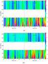 |
Fig. 12. Phase solutions ϕ in radians in LBA and HBA for the two stations RS205 and RS509 as a function of time (x-axis) and frequency (y-axis). Panel a: solutions towards calibrator direction dir36, panel b: towards dir100. |
5.4. Calibration scenarios for LOFAR 2.0
To study possible scenarios of direction-dependent calibration in LOFAR 2.0, we rely on strategies which extract the TEC from the direction-dependent phase solutions. We use the software LoSoTo (de Gasperin et al. 2019) to fit the dispersive-delay term (see Eq. (2)). To reduce the local minima problem, a grid-search is performed to determine the initial guess of the optimization. We assign a weight to the LBA phase solutions according to w(ν) = min(SEFD)/SEFD(ν), the HBA phase solutions are assigned a constant weight of w = 1. We compare three different approaches to extract dTEC from the phase-solutions: First, using only the LBA solutions, as shown in Figs. 13a and b. Second, using only the HBA solutions, as shown in Figs. 13c and d. This scenario is the case of solution-transfer. Third, testing joint calibration – we combine LBA and HBA solutions to extract TEC over a broad frequency range, see Figs. 13e and f.
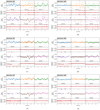 |
Fig. 13. Direction-dependent TEC-solutions (colors except red) and residuals with respect to the simulation input (red) shown in each of the six panels a–f for six distant RS. Residuals outside of the displayed range are indicated by arrows. Panels a, c, and e: in the left column show solutions towards dir36, whereas panels b, d, and f: in the right column show solutions towards dir100. In the two figures a and b in the top row, only LBA phase solutions were used to extract the dTEC, while for the center row c, d, only HBA was considered. The figures e and f in the bottom row show joint calibration solutions derived from LBA and HBA combined. The gray lines in the background of the dTEC panels show the difference between input dTEC and direction-independent dTEC solutions for this station and direction, these values were used to calculate the residuals as dTECresidual = dTECDDE − (dTECinput − dTECDIE). All values are referenced to CS001LBA and CS001HBA0, respectively. |
Due to the different beam sizes, the direction-independent TEC-solution of LBA and HBA differ slightly. Therefore, the direction-dependent solutions will also be slightly different to account for this offset. Thus, direction-independent solutions obtained with one antenna type cannot directly be combined with direction-dependent solutions obtained with the other. We take this into account by applying the HBA direction-independent solutions for the remote stations to the LBA data in the first and second case. For the third case, we also add the phases corresponding to the difference between the HBA and LBA direction-independent TEC solutions to the direction-dependent phase solutions in LBA to establish a common ground for direction-dependent TEC-extraction. The results of all three approaches as well as the residuals with respect to the simulation input are displayed in Fig. 13 for the calibrators dir36 and dir100. In Fig. 14, we show the rms error of the TEC solutions for the six calibration directions and all remote stations. In the LBA only case, while many of the residuals are close to zero, a substantial fraction converged towards neighboring minima, leading to a rms error which is, in most cases, higher than in the competing approaches. This can be explained with the low S/N of the LBA. For the HBA observation, most stations and directions reach a mTECU-scale rms error but show a small systematic offset in the residuals. This offset appears to be present in most directions to a similar extent, pointing towards a direction-independent phase error in the data which is not fully corrected. One negative exception is the complex source dir64, where no sufficiently accurate model could be derived in HBA, leading to significantly noisier solutions. Further parameter fine-tuning could potentially improve solutions for this direction. Furthermore, for station RS310, improper solutions were found during direction-independent calibration. This issue propagates to direction-dependent calibration. In the joint-calibration approach, the mean rms of the solutions is the lowest and the aforementioned issues are partially solved. The TEC-jumps are considerably less frequent than in the LBA-only case, the systematic drifts present in the HBA residuals are attenuated and the solutions for the problematic station RS310 are substantially improved compared to the HBA-only case.
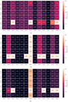 |
Fig. 14. Each of the three panels a–c: direction-dependent TEC rms error as a function of direction (y-axis) and station (x-axis). The TEC was extracted from phase solutions derived from LBA (a), HBA, (b) or both (c). |
In Fig. 15, we show LBA images of the six calibrators, comparing image quality without direction-dependent corrections to the three different direction-dependent calibration strategies of our analysis. In all cases, the image quality improved compared to the direction-independently calibrated image. The best image quality is achieved using either LBA or joint-calibration TEC solutions, both approaches result in a noise level of 0.9 mJy beam. The characteristic star-like patterns around the sources caused by the ionospheric dispersive delay are removed almost completely. However, extended, spiral-shaped artifacts remain. The image quality using only the LBA stations for calibration is equally good and for some directions even slightly better than the joint calibration despite the joint-calibration solutions being more accurate. This can be explained by two points: first, the jumps in LBA-extracted TEC lead to a high rms of the residuals while still providing a decent calibration for part of the frequency band, and second, remaining corruptions in the LBA data might not be fully described by a TEC-term.
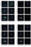 |
Fig. 15. 12″-region around the six calibrator directions used in the analysis with different calibration solutions applied shown in panels a–d. All images share the same color scale and show LBA data centered at 54 MHz. Panel a: is corrected only for direction-independent effects, panels b and c: are corrected using TEC-solutions derived from only LBA or only HBA, and panel d: joint-calibration case. |
Image quality is worse in the solution-transfer scenario: noticeable calibration artifacts are present, revealing that multiple stations are not well calibrated. This gives rise to the question of why the image quality in this scenario is inferior if the solutions show fewer jumps than the ones obtained from LBA. The explanation for this must lie in the systematic offsets which can be observed in the HBA residuals in Fig. 13. The likely cause of these offsets comes from a phase error in HBA that was not fully corrected by our calibration strategy; however, the root of this issue could not be determined. While the HBA TEC-solutions will certainly improve if the phase offset can be solved, this also highlights an intrinsic disadvantage of the solution-transfer approach: while the presence of small phase errors in HBA data can still lead to satisfying results using TEC-calibration at HBA frequencies, transferring the solutions to LBA can strongly amplify any phase errors from TEC-offsets. Even if there were no residual errors in the simulated data, minor systematic effects which are not present in the simulation could cause similar problems in real observations. Therefore, solution-transfer is only viable if the HBA data are free of non-ionospheric phase errors.
A more refined calibration strategy could improve the solutions obtained during direction-dependent calibration. Most notably, we emphasize that there are further points were the simultaneity of the observations could be exploited. It would be possible to jointly calibrate the first, second, and possible third order ionospheric term as well as clock delays during direction-independent calibration. Additionally, the spectral properties of the model components could be estimated more accurately by a unified model for the low and high band, possibly obtained by joint de-convolution.
To use joint calibration strategies in application in the future, the development of specialized software will be necessary. Possible advancements include the implementation of a solution algorithm which can solve for TEC and further frequency-dependent effects on LBA and HBA data together, bypassing the intermediate phase-solution. Furthermore, joint calibration could enable the leap from facet-based towards TEC-screen based calibration as proposed in Albert et al. (2020) in LOFAR 2.0 by increasing the robustness of the TEC-estimates towards residual phase errors.
5.5. Limitations
A number of points must be considered when evaluating the accuracy of LoSiTo simulations. First of all, only the first and second order ionospheric effects are implemented in the simulation. Higher-order effects are non-negligible at the lowest frequencies observed by LOFAR (ν ≲ 40 MHz). Additionally, in real LOFAR observations, the presence of ionospheric scintillation can affect the coherency of celestial radio signals under special ionospheric conditions. These scintillations, together with artificial radio-frequency interference (RFI), can render data unusable for periods of time, but are not accounted for in LoSiTo. Second, while we do not expect the thin-layer and frozen turbulence assumptions to interfere with facet-based calibration strategies, we need to be cautious in using the simulations when working with approaches that enforce spatial coherency across multiple stations, since the phase error from projecting the three-dimensional structure onto a two-dimensional layer is not represented. Third, the simulated sky cannot recreate the complexity of the real radio sky due to limitations in computing power. The sky model used in this work underestimates the number density especially of faint sources. Furthermore, it does not contain emission in side lobes or on very large angular scales, both of which are known to interfere with calibration (de Gasperin et al. 2020; Shimwell et al. 2017). Fourth, the beam model employed in the simulation is the product of semi-analytic simulations. It is known that the real beam response deviates from this model to some extent (de Gasperin et al. 2019). This deviation is not included in the simulation. Last, real LOFAR data can contain subdominant systematic effects that are not well understood at present and hence, cannot be modeled in simulations.
6. Conclusions
In this paper, we present models for a comprehensive list of systematic effects in LOFAR and LOFAR 2.0 observations and the LoSiTo code in which we embedded them. These models include a turbulent thin-layer representation of the ionosphere which is used to derive the first and second order ionospheric effect. Furthermore, LoSiTo features the systematic effects of clock error, polarization misalignment, the primary beam and bandpass responses as well as an estimate of the LOFAR 2.0 noise level based on empirically determined values for the LOFAR SEFD. The product of a simulation is a “measurement set”, which can be further processed with standard radio astronomy tools. The code was developed with the aim to assist the progression of current and future LOFAR calibration strategies and has been made publicly available.
We used LoSiTo to simulate a full eight-hour calibrator and target field observation using the LOFAR 2.0 system. We presented the analysis of the simulated data, where we performed data reduction of the calibrator observation and direction-dependent calibration of the target field using adjusted LOFAR calibration pipelines. As a proof-of-concept, we investigated new strategies for direction-dependent calibration of the data. We compared ionospheric solutions derived from LBA and HBA separately to solutions derived jointly from both systems. We found that the ionospheric parameters of the simulation can be determined most accurately in the joint calibration approach, where we reach a mTEC-scale rms error in 90% of the cases. When we use only LBA data for calibration, the solutions are more noisy; nevertheless, the resulting image quality is very similar to the joint calibration approach with an rms noise of 0.9 mJy beam away from bright sources and artifacts in the vicinity of the calibrators. This indicates that while we managed to determine the TEC accurately, our image-space results are still limited by the presence of systematic errors which could be resolved by an improvement of the strategy. For the case of solution transfer, where the ionospheric solutions found in the HBA calibration are applied to the LBA data, we find good convergence and very little noise in the solutions. However, they show systematic offsets at a scale of ≈5 mTECU which create strong artifacts in image-space. While further development of the calibration procedure could improve the image quality, this result reveals a central downside of the solution-transfer approach: errors in the HBA data are strongly amplified when the solutions are applied to LBA data. Therefore, solution transfer can only be an option if all non-ionospheric effects in HBA are corrected to a high level of accuracy.
Derived from the phase structure function spectral index α as β = α − 2 according to Boreman & Dainty (1996).
Acknowledgments
We thank the anonymous referee for their constructive remarks on this work. This project is funded by the Deutsche Forschungsgemeinschaft (DFG, German Research Foundation) under projet number 427771150. The authors thank J. Hessels, C. Bassa, T. Shimwell and the LOFAR 2.0 developing team for their help.
References
- Albert, J. G., van Weeren, R. J., Intema, H. T., & Röttgering, H. J. A. 2020, A&A, 635, A147 [CrossRef] [EDP Sciences] [Google Scholar]
- Bilitza, D. 2018, Adv. Radio Sci., 16, 1 [CrossRef] [Google Scholar]
- Boreman, G., & Dainty, C. 1996, J. Opt. Soc. Am. A, 13, 517 [CrossRef] [Google Scholar]
- Buscher, D. F. 2016, Opt. Exp., 24, 23566 [CrossRef] [Google Scholar]
- Chulliat, A., Macmillan, S., Alken, P., et al. 2015 The US/UK World Magnetic Model for 2015-2020: Tech. Rep., National Geophysical Data Center, NOAA, https://www.doi.org/10.7289/V5TB14V7 [Google Scholar]
- Datta-Barua, S., Walter, T., Blanch, J., & Enge, P. 2008, Radio Sci., 43, RS5010 [NASA ADS] [CrossRef] [Google Scholar]
- de Gasperin, F., Mevius, M., Rafferty, D. A., Intema, H. T., & Fallows, R. A. 2018, A&A, 615, A179 [NASA ADS] [CrossRef] [EDP Sciences] [Google Scholar]
- de Gasperin, F., Dijkema, T. J., Drabent, A., et al. 2019, A&A, 622, A5 [NASA ADS] [CrossRef] [EDP Sciences] [Google Scholar]
- de Gasperin, F., Brunetti, G., Brüggen, M., et al. 2020, A&A, 642, A85 [CrossRef] [EDP Sciences] [Google Scholar]
- de Gasperin, F., Williams, W. L., Best, P., et al. 2021, A&A, 648, A104 [CrossRef] [EDP Sciences] [Google Scholar]
- Dewdney, P. E., Hall, P. J., Schilizzi, R. T., & Lazio, T. J. L. W. 2009, IEEE Proc., 97, 1482 [Google Scholar]
- Dutch Research Council (NWO) 2018, NWO Investment Grant Large 2017–2018 [Online; accessed 12. Oct. 2020] [Google Scholar]
- Giannattasio, F., De Michelis, P., Consolini, G., et al. 2018, Ann. Geophys., 61 [CrossRef] [Google Scholar]
- Guzmán, A. E., May, J., Alvarez, H., & Maeda, K. 2011, A&A, 525, A138 [NASA ADS] [CrossRef] [EDP Sciences] [Google Scholar]
- Hamaker, J. P. 2011, Mathematical-Physical Analysis of the Generic Dual-Dipole Antenna, Tech. Rep., ASTRON [Google Scholar]
- Hamaker, J. P., Bregman, J. D., & Sault, R. J. 1996, A&AS, 117, 137 [NASA ADS] [CrossRef] [EDP Sciences] [Google Scholar]
- Lipiński, M., Włostowski, T., Serrano, J., & Alvarez, P. 2011, 2011 IEEE International Symposium on Precision Clock Synchronization Measurement, Control and Communication, 25 [CrossRef] [Google Scholar]
- Mahony, E. K., Morganti, R., Prandoni, I., et al. 2016, MNRAS, 463, 2997 [NASA ADS] [CrossRef] [Google Scholar]
- Martin, P. L., Bray, J. D., & Scaife, A. M. M. 2016, MNRAS, 459, 3525 [CrossRef] [Google Scholar]
- Materassi, M., Forte, B., Coster, A., & Skone, S. 2019, The Dynamical Ionosphere – A Systems Approach to Ionospheric Irregularity, 1st edn. (Netherlands: Elsevier), 301 [Google Scholar]
- Mevius, M. 2018a, in Low Frequency Radio Astronomy and the LOFAR Observatory, eds. J. M. George Heald, & R. Pizzo (Springer), 103 [NASA ADS] [CrossRef] [Google Scholar]
- Mevius, M. 2018b, Astrophysics Source Code Library [record ascl:1806.024] [Google Scholar]
- Mevius, M., van der Tol, S., Pandey, V. N., et al. 2016, Radio Sci., 51, 927 [Google Scholar]
- Mohan, N., & Rafferty, D. 2015, Astrophysics Source Code Library [record ascl:1502.007] [Google Scholar]
- Offringa, A. R., & Smirnov, O. 2017, MNRAS, 471, 301 [NASA ADS] [CrossRef] [Google Scholar]
- Offringa, A. R., McKinley, B., Hurley-Walker, N., et al. 2014, MNRAS, 444, 606 [NASA ADS] [CrossRef] [Google Scholar]
- Schoenmaker, A. P., & Renting, G. A. 2011, MS2 Description for LOFAR [Google Scholar]
- Shimwell, T. W., Röttgering, H. J. A., Best, P. N., et al. 2017, A&A, 598, A104 [NASA ADS] [CrossRef] [EDP Sciences] [Google Scholar]
- Smirnov, O. M. 2011, A&A, 527, A106 [NASA ADS] [CrossRef] [EDP Sciences] [Google Scholar]
- Tasse, C., Shimwell, T., Hardcastle, M. J., et al. 2021, A&A, 648, A1 [EDP Sciences] [Google Scholar]
- Tatarski, V. I. 1961, Wave Propagation in a Turbulent Medium, Translated by R. A. Silverman (New York: McGraw-Hill) [Google Scholar]
- Tatarski, V. I. 1971, Nauka Press, Moscow (in Russian; English Translation: National Technical Information Service, Springfield, Va., 1971) [Google Scholar]
- Taylor, G. B., Carilli, C. L., Perley, R. A., et al. 1999, Synthesis Imaging in Radio Astronomy II (Astronomical Society of the Pacific), 170 [Google Scholar]
- Taylor, G. B., Ellingson, S. W., Kassim, N. E., et al. 2012, J. Astron. Instrum., 1, 1250004 [CrossRef] [Google Scholar]
- Thompson, A. R., Moran, J. M., & Swenson, G. W. 2017, Interferometry and Synthesis in Radio Astronomy, 3rd edn. (Springer) [Google Scholar]
- Tingay, S. J., Goeke, R., Bowman, J. D., et al. 2013, PASA, 30, e007 [Google Scholar]
- van Cappellen, W. 2019, LOFAR 2.0 Stage 1 Development, Talk at LOFAR Science Workshop 2019 [Google Scholar]
- van Diepen, G., Dijkema, T. J., & Offringa, A. 2018, Astrophysics Source Code Library [record ascl:1804.003] [Google Scholar]
- van Haarlem, M. P., Wise, M. W., Gunst, A. W., et al. 2013, A&A, 556, A2 [NASA ADS] [CrossRef] [EDP Sciences] [Google Scholar]
- van Weeren, R. J., Williams, W. L., Hardcastle, M. J., et al. 2016, ApJS, 223, 2 [NASA ADS] [CrossRef] [Google Scholar]
- von Karman, T. 1948, Proc. Natl. Acad. Sci., 34, 530 [CrossRef] [Google Scholar]
All Tables
Numeric values for the widths of the Gaussian distributions used to construct the LOFAR 2.0 clock model.
All Figures
|
Fig. 1. Snapshot of a simulated turbulent TEC-screen with the parameters β = 3.89 and hiono = 250 km. Each circle marks one pierce-point, circles of the same color show pierce-points for different directions belonging to the same station. Only pierce-points belonging to one of the centermost stations (CS001), the most distant central station (CS501) as well as the three outermost remote stations (RS210, RS310, RS509) are displayed. |
| In the text | |
|
Fig. 2. Simulated dTEC (top panels) and dRM (bottom panels) for three stations for a source in the phase center (orange) and for sources separated from the phase center by 1.75° (blue) and 4.51° (green). The stations are at distances of 1.7 km (CS501), 6.3 km (RS205) and 55.7 km (RS509) to CS001. The values of each direction are referenced with respect to the same direction in CS001LBA. |
| In the text | |
|
Fig. 3. Normalized LOFARBeam beam response (y-axis) as a function of phase center separation (x-axis) for the current 48 dipole LBA system in mode outer, the 96 dipole LOFAR 2.0 LBA system and the HBA system. The dashed vertical lines mark the primary beam FWHM of the respective system. |
| In the text | |
|
Fig. 4. Normalized bandpass amplitudes (y-axis) for the LBA and the most common HBA bandpass setup HBA-low as a function of frequency (x-axis). The values are adopted from an empirical study of the instrument in van Haarlem et al. (2013). |
| In the text | |
|
Fig. 5. Simulated clock delay for CS501 (blue), RS205 (orange), and RS210 (green), referenced to the clock of CS001. |
| In the text | |
|
Fig. 6. Frequency dependence of the SEFD for different configurations of the LBA (left) and two differently equipped HBA station types (right). The estimate for the LOFAR 2.0 LBA SEFD is derived from the mean of the modes Inner and Outer. |
| In the text | |
|
Fig. 7. Diagram of LoSiTo. As input, a parameter set, a sky model, and a template measurement set are required. Orange boxes represent DDE, while yellow boxes represent DIE. |
| In the text | |
|
Fig. 8. Input sky model of the simulation. The model is extracted from a real LOFAR observation of the target field. It contains 340 sources grouped into 59 patches, the total flux density is 226 Jy at 56 MHz. Circles correspond to source locations. Sources are color-coded according to their patch membership, patch centers are marked by an “X” and labeled. |
| In the text | |
|
Fig. 9. Direction-independent ionospheric solutions towards the target field for four LBA stations. Top panels: dTEC, the bottom panels dRM. The gray curves in the background show the input corruptions towards the 59 patches. The calibration solutions are referenced to station CS001LBA and the input corruptions are referenced to the phase center direction of CS001LBA. Triangles mark solutions outside of the graph’s scale. We note that the missing variation of the input-RM for CS001 is caused by a referencing error present in the data. Simulated RM values were referenced for each direction individually instead of referencing to a single direction. However, we do not expect this to affect our analysis. |
| In the text | |
|
Fig. 10. Direction-independent TEC solutions for four HBA stations. The gray curves in the background show the input corruptions towards the 59 patches. The calibration solutions are referenced to station CS001HBA0. The input corruptions are referenced to the phase center direction of CS001HBA0. |
| In the text | |
|
Fig. 11. LBA wide-field image after DIE calibration. The rms background noise is ≈2.0 mJy beam−1 at a resolution of 42″ × 30″. The DDE calibrator directions are highlighted in red, the blue dashed circles show the primary beam FWHM of the LOFAR 2.0 LBA at 54 MHz and the HBA at 144 MHz. The background color scale shows the logarithmic surface brightness in arbitrary units. |
| In the text | |
|
Fig. 12. Phase solutions ϕ in radians in LBA and HBA for the two stations RS205 and RS509 as a function of time (x-axis) and frequency (y-axis). Panel a: solutions towards calibrator direction dir36, panel b: towards dir100. |
| In the text | |
|
Fig. 13. Direction-dependent TEC-solutions (colors except red) and residuals with respect to the simulation input (red) shown in each of the six panels a–f for six distant RS. Residuals outside of the displayed range are indicated by arrows. Panels a, c, and e: in the left column show solutions towards dir36, whereas panels b, d, and f: in the right column show solutions towards dir100. In the two figures a and b in the top row, only LBA phase solutions were used to extract the dTEC, while for the center row c, d, only HBA was considered. The figures e and f in the bottom row show joint calibration solutions derived from LBA and HBA combined. The gray lines in the background of the dTEC panels show the difference between input dTEC and direction-independent dTEC solutions for this station and direction, these values were used to calculate the residuals as dTECresidual = dTECDDE − (dTECinput − dTECDIE). All values are referenced to CS001LBA and CS001HBA0, respectively. |
| In the text | |
|
Fig. 14. Each of the three panels a–c: direction-dependent TEC rms error as a function of direction (y-axis) and station (x-axis). The TEC was extracted from phase solutions derived from LBA (a), HBA, (b) or both (c). |
| In the text | |
|
Fig. 15. 12″-region around the six calibrator directions used in the analysis with different calibration solutions applied shown in panels a–d. All images share the same color scale and show LBA data centered at 54 MHz. Panel a: is corrected only for direction-independent effects, panels b and c: are corrected using TEC-solutions derived from only LBA or only HBA, and panel d: joint-calibration case. |
| In the text | |
Current usage metrics show cumulative count of Article Views (full-text article views including HTML views, PDF and ePub downloads, according to the available data) and Abstracts Views on Vision4Press platform.
Data correspond to usage on the plateform after 2015. The current usage metrics is available 48-96 hours after online publication and is updated daily on week days.
Initial download of the metrics may take a while.