| Issue |
A&A
Volume 653, September 2021
|
|
|---|---|---|
| Article Number | A87 | |
| Number of page(s) | 20 | |
| Section | Interstellar and circumstellar matter | |
| DOI | https://doi.org/10.1051/0004-6361/202040262 | |
| Published online | 13 September 2021 | |
The TOPGöt high-mass star-forming sample
I. Methyl cyanide emission as tracer of early phases of star formation★
1
Dipartimento di Fisica e Astronomia, Universitá degli Studi di Firenze,
Via Sansone 1,
50019
Sesto Fiorentino,
Italy
e-mail: chiara.mininni@inaf.it
2
INAF Osservatorio Astrofisico di Arcetri,
Largo E. Fermi 5,
50125
Firenze,
Italy
3
Istituto di Astrofisica e Planetologia Spaziali, INAF,
Via Fosso del Cavaliere 100,
00133
Roma,
Italy
4
I. Physikalisches Institut, Universität zu Köln,
Zülpicher Str. 77,
50937
Köln,
Germany
5
Centro de Astrobiología (CSIC, INTA),
Ctra. de Ajalvir, km. 4, Torrejón de Ardoz,
28850
Madrid,
Spain
6
Department of Physical Science, Graduate School of Science, Osaka Prefecture University,
1-1 Gakuen-cho, Naka-ku, Sakai,
Osaka
599-8531,
Japan
7
National Astronomical Observatory of Japan, National Institutes of Natural Science,
2-21-1 Osawa,
Mitaka,
Tokyo
181-8588,
Japan
8
Joint Institute for VLBI ERIC,
Oude Hoogeveensedijk 4,
7991
PD Dwingeloo,
The Netherlands
9
Leiden Observatory, Leiden University,
Postbus 9513,
2300 RA
Leiden,
The Netherlands
10
INAF, Istituto di Radioastronomia, Italian ARC,
Via P. Gobetti 101,
Bologna,
Italy
11
Max-Planck-Institut für Extraterrestrische Physik,
Gießenbachstraße 1,
85748
Garching bei München,
Germany
12
European Southern Observatory (ESO),
Karl-Schwarzschild-Str. 2,
85748
Garching,
Germany
13
Excellence Cluster Origins,
Boltzmannstrasse 2,
85748
Garching bei München,
Germany
Received:
30
December
2020
Accepted:
14
July
2021
Aims. The TOPGöt project studies a sample of 86 high-mass star-forming regions in different evolutionary stages from starless cores to ultra compact HII regions. The aim of the survey is to analyze different molecular species in a statistically significant sample to study the chemical evolution in high-mass star-forming regions, and identify chemical tracers of the different phases.
Methods. The sources have been observed with the IRAM 30 m telescope in different spectral windows at 1, 2, and 3 mm. In this first paper, we present the sample and analyze the spectral energy distributions (SEDs) of the TOPGöt sources to derive physical parameters such as the dust temperature, Tdust, the total column density, NH2, the mass, M, the luminosity, L, and the luminosity-to-mass ratio, L∕M, which is an indicator of the evolutionary stage of the sources. We use the MADCUBA software to analyze the emission of methyl cyanide (CH3CN), a well-known tracer of high-mass star formation.
Results. We built the spectral energy distributions for ~80% of the sample and derived Tdust and NH2 values which range between 9−36 K and ~3 × 10²¹−7 × 1023 cm−2, respectively. The luminosity of the sources spans over four orders of magnitude from 30 to 3 × 10⁵ L⊙, masses vary between ~30 and 8 × 10³ M⊙, and the luminosity-to-mass ratio L∕M covers three orders of magnitude from 6 × 10⁻² to 3 × 10² L⊙∕M⊙. The emission of the CH3CN(5K-4K) K-transitions has been detected toward 73 sources (85% of the sample), with 12 nondetections and one source not observed in the frequency range of CH3CN(5K-4K). The emission of CH3CN has been detected toward all evolutionary stages, with the mean abundances showing a clear increase of an order of magnitude from high-mass starless cores to later evolutionary stages. We found a conservative abundance upper limit for high-mass starless cores of XCH3CN < 4.0 × 10⁻¹¹, and a range in abundance of 4.0 × 10⁻¹¹ < XCH3CN < 7.0 × 10⁻¹¹ for those sources that are likely high-mass starless cores or very early high-mass protostellar objects. In fact, in this range of abundance we have identified five sources previously not classified as being in a very early evolutionary stage. The abundance of CH3CN can thus be used to identify high-mass star-forming regions in early phases of star-formation.
Key words: astrochemistry / ISM: molecules / stars: formation / stars: massive
Full Tables 3–6 are only available at the CDS via anonymous ftp to cdsarc.u-strasbg.fr (130.79.128.5) or via http://cdsarc.u-strasbg.fr/viz-bin/cat/J/A+A/653/A87
© ESO 2021
1 Introduction
High-mass star-forming regions, the cradles of high-mass stars (M > 8 M⊙), are among the most chemically rich sources in the Galaxy (e.g., Belloche et al. 2019). Despite their relatively low number, these regions havea deep impact on the physical and chemical evolution of their surroundings and on the evolution of the Galaxy itself (Motte et al. 2018).
A unique scenario for the formation of high-mass stars has not been found yet. Several models have been proposed to overcome the theoretical problem that arises from the fact that protostars with masses larger than 8 M⊙ reach the main sequence before the end of the accretion process, and that the radiation emitted by the newborn star would halt accretion (McKee & Tan 2003; Bonnell & Bate 2006; Keto 2007; Krumholz et al. 2009; Motte et al. 2018). Even if a conclusive theory describing the evolutionarysequence of high-mass star-forming regions has not been defined yet, an empirical rough classification has been proposed (Beuther et al. 2007; Motte et al. 2018). The earliest stage is represented by high-mass starless cores (HMSCs), with a high H2 volume density (n ~ 105 cm−3) and low kinetic temperatures T ~ 15 K, for which noevidence of ongoing star-formation (i.e., powerful outflows, strong IR sources, and/or masers) is present. This stage is followed by that of high-mass protostellar objects (HMPOs), where an accreting protostar is already present and visible at wavelengths of 20−70 μm, even if it is still embedded in the natal cloud. HMPOs are warmer than HMSCs, reaching temperatures of a few hundred kelvins close to the central protostar(s). In these conditions, the molecules frozen onto dust grains are released in the gas phase enriching the gas chemistry and leading to the formation of the so-called hot molecular cores (HMCs). The last evolutionary stage is represented by ultra compact HII regions (UC HIIs), in which the UV photons from the central protostar have ionized the surrounding gas, creating a photoionized compact region (diameter ≲ 0.1 pc), visible at centimeter wavelengths due to free-free emission.
It is of particular interest in the field of astrochemistry to characterize the evolution of the chemistry along these evolutionarystages. This will increase the knowledge of the chemical features characterizing each stage, which in turn can shed light on the physical processes that take place, and help to constrain the physical evolution. To reach this goal, it is important to analyze statistically significant samples in order to derive general properties for each evolutionarystage not influenced by possible peculiarities of a single source. For this reason, we ideated the TOPGöt project1 : the project unites, in the vision of a combined effort, the observations made with the IRAM 30 m telescope at 1, 2, and 3 mm toward two already statistically significant samples of high-mass star-forming regions (presented in Sect. 2) for a total of 86 sources covering all three evolutionary stages described above. Table 1 lists the spectral windows observed toward the two subsamples, with examples of molecular species covered by each frequency range.
In this paper, we first introduce the sample and focus on the characterization of the physical properties of the sources, analyzing their spectral energy distributions (SEDs) to derive the dust temperature, Tdust, the H2 column density,  , the mass, M, and the luminosity, L, of the sources. TheH2 column density allows us to derive the molecular abundances, while the other observables allow us to search for (anti)correlations between chemical abundances and physical properties of the sources. Following the SED analysis, we characterize the emission of methyl cyanide (CH3CN) in the (5K −4K) rotational transition, a well-known high-density tracer in high-mass star-forming regions (e.g., Churchwell et al. 1992). This molecule, firstly detected in its (6K −5K) transition toward the Galactic Center by Solomon et al. (1971), is a symmetric top and its transitions are characterized by the two quantum numbers J, the total angular momentum, and K, the projection of the total angular momentum on the symmetry axis. Since quantum mechanic selection rules allow only ΔJ = ± 1 and ΔK = 0 transitions, the population of the different K components can be used to infer a reliable estimate of the kinetic temperature. The analysis of methyl cyanide is also favored by the fact that the lines with different K in a given rotational transition are separated by a few MHz (see Table 2), that is much less than the bandwidth of any spectrometer available at modern radio telescopes. Therefore, these different K-components can be observed simultaneously in the same spectral window, and their intensities are independent of relative calibration uncertainties.
After its first detection several studies detected methyl cyanide in high-mass star-forming regions (Bergman & Hjalmarson 1989; Churchwell et al. 1992; Olmi et al. 1993, 1996a; Zhang et al. 1998; Kalenskii et al. 2000; Pankonin et al. 2001; Remijan et al. 2004; Araya et al. 2005; Purcell et al. 2006; Rosero et al. 2013; Minh et al. 2016; Hung et al. 2019)showing emission associated with HMPOs and UC HII regions. Olmi et al. (1996b), with interferometric observations, and Giannetti et al. (2017b), observing a large sample of cores (including HMSCs), found that, while high-energy K components of methyl cyanide trace only the most compact and warmer cores, low-energy K components trace also more extended and colder gas. Other high-angular resolution studies have highlighted that methyl cyanide is a good tracer of rotating toroids and infall in high-mass protostars (Cesaroni et al. 1999; Beltrán et al. 2004, 2005, 2011a, 2018; Furuya et al. 2008). Finally, this species has also been found in gas affected by the passage of a shock wave, as in L1157-B1 (Arce et al. 2008; Codella et al. 2009), in circumstellar envelopes of evolved stars (i.e., Agúndez et al. 2015), in disks (Öberg et al. 2015; Johnston et al. 2015; Bergner et al. 2018; Loomis et al. 2018), and cold dense cores (e.g., Potapov et al. 2016; Spezzano et al. 2017).
The paper is structured as follows: in Sect. 2 we present the sample and its selection criteria. In Sect. 3 we describe the observations of the CH3CN(5K−4K) lines with the IRAM 30 m telescope. In Sect. 4 we present the analysis of the SEDs toward the 86 objects in the sample, how we derived the physical quantities of Tdust,  , L and M, and the analysis of the methyl cyanide (5K−4K) rotational transitions. In Sect. 5 we discuss the results. Finally in Sect. 6 we summarize the conclusions.
Spectral windows observed toward Subsample I and Subsample II.
Parameters of the K-ladder of CH3CN(5−4).
2 The sample
The sample of the TOPGöt project arises from the combination of two separate subsamples of high-mass star-forming regions containing 86 targets in total.
2.1 Subsample I
The first subsample (hereafter Subsample I), firstly presented in Fontani et al. (2011), consists of 27 sources (~31% of the total sample) for which we already have an evolutionary classification: 11 are HMSCs, 9 are HMPOs, and 7 are UC HII regions.
2.1.1 Selection criteria for HMSCs
The HMSCs have been selected as massive cores embedded in infrared dark-clouds or other massive star-forming regions in which no evidence of ongoing star formation was present. Fontani et al. (2011) checked that no embedded infrared sources, powerful outflows or maser emission were detected toward these sources. Later, Tan et al. (2016) found that a source classified as HMSC, G028-C1, is associated with a highly ordered outflow. However, given that this outflow is still in an initial phase with no powerful emission and that the source shows bright emission of N2D+(3–2), which is a tracer of dense and cold gas of prestellar cores (as discussed in Tan et al. 2016), we decided to still classify G028-C1 as HMSC. In fact, the three different classes are not sharply separated, and all the other observational parameters checked for this source are more similar to those of other objects classified as HMSCs than those of HMPOs. Among the HMSCs, three sources (AFGL5142-EC, 05358-mm3, and I22134-G) have been defined as “warm” (HMSCw), since they have temperatures Tk > 20 K (see Table A.3 of Fontani et al. 2011), derived from ammonia rotation temperatures following Tafalla et al. (2004). This is confirmed by high-angular resolution studies that indicate that they could be externally heated by nearby protostellar objects (Zhang et al. 2002; Busquet et al. 2010; Sánchez-Monge et al. 2011; Colzi et al. 2019).
2.1.2 Selection criteria for HMPOs and UC HII regions
HMPOs have been selected as high-mass sources associated with infrared sources, and/or powerful outflows and/or faint (Sν at 3.6 cm < 1 mJy) radio continuum emission likely tracing a thermal radio jet. UC HIIs are associated with strong radio continuum emission (Sν at 3.6 cm ≥ 1 mJy) tracing gas ionized by the UV photons emitted by a young massive star. More evolved sources, in which HII regions have already dissipated the associated molecular cores, were not included.
A small part of the observations toward these sources has already been analyzed and published in previous works covering different topics, from deuteration in selected molecules (N2H+, CH3OH, NH3, HC3N; Fontani et al. 2011, 2015a; Rivilla et al. 2020), to nitrogen fractionation of HCN, HNC and N2H+ (Fontani et al. 2015b; Colzi et al. 2018a), to prebiotic and complex organic molecules (COMs, Mininni et al. 2018; Coletta et al. 2020).
2.2 Subsample II
The second subsample (hereafter Subsample II) consists of 59 high-mass star-forming regions (~69% of the total sample) located in the northern hemisphere. The sources were identified from a number of available mm-continuum emission surveys of star-forming regions (Molinari et al. 1996; Beuther et al. 2002; Mueller et al. 2002; Sridharan et al. 2002; Sánchez-Monge et al. 2008), with the goal of studying the chemical evolution of star-forming regions and statistically search for the presence of chemically rich hot molecular cores. The sources were selected primarily based on two aspects: (i) sources with kinematic distances2 ≤ 5.5 kpc, to reduce beam-dilution effects and therefore increase the probability to detect molecular emission, and (ii) presence of a bright and dense gas and dust condensation, mainly evaluated on the basis of bright peak intensities (≥ 0.5 Jy beam−1) at millimeter wavelengths, suggestive of high-mass young stellar objects embedded in dust.
For the sources in Subsample II a previous evolutionary classification has not been performed yet, however we expect that most of the sources are in the evolutionary stages of HMPOs or UC HII regions, from criterion (ii). A first attempt of classification based on the abundances of methyl cyanide, together with other evolutionary indicators, will be presented in Sect. 5.
The two subsamples have been separately observed in several spectral windows with the IRAM 30 m telescope, leading to a collection of ancillary data covering the range of emission of several molecular species (Table 1). Since the observed spectral windows of Subsample II overlap with the spectral windows of Subsample I, it was decided to carry out this project by merging the two samples to increase the statistical value of this study. Moreover, the project will include future studies on other molecular species detected in the available ancillary data. Thus, this paper is also a reference paper for the project, where we characterize some important physical properties of the sources needed for the analysis of the molecular emission of different species.
The merged sample has been already used to study the nitrogen fractionation in HCN and HNC by Colzi et al. (2018b). The coordinates of the sources, the distance d, the velocity vLSR, and the evolutionary classification are given in Table 3. The sources belonging to Subsample I are those that have an evolutionary classification, while for sources of Subsample II the last column in Table 3 is empty. All the d are kinematic distances, with the exception of the distance estimate of G31.41+0.31 and G35.20-0.74 that are derived from parallax measurements (Immer et al. 2019; Zhang et al. 2009). When the distance ambiguity was not resolved (14% of the full sample, 17% of the sources with SED, and 14% of the sources for which we detected CH3CN) we adopted the near distance. Since only in a low percentage of the sample the distance ambiguity is not resolved, this does not affect the interpretation of the data and the results, especially considering that in part of the discussion we make use of distance-independent parameters.
Sources coordinates, heliocentric distances, line-of-sight velocities, and evolutionary phases (e.p.).
3 Observations
The observations of the CH3CN(5K–4K) transition toward the Subsample I analyzed in this work are taken from the dataset described in Fontani et al. (2015a), but have not been previously analyzed. Due to time constraints the source G028-C3(MM11) was not observed in the run targeting the CH3CN(5K−4K) lines. However, this source is presented in this paper since the derivation of the physical parameters from the SED will be needed to analyze observations of other species, presented in future papers. More details about the observations toward Subsample I can be found in Fontani et al. (2015a).
The sources in Subsample II were observed using the IRAM 30 m telescope from 11 to 16 August 2014 (project 040-14, PI: Sánchez-Monge). We simultaneously observed two bands at 3 and 2 mm covering some important rotational transitions of common species such as HCO+, HCN, HNC, N2H+ and SiO, as well as transitions of complex organic molecules such as CH3CN and CH3OH. The observed frequencies are 85.7–93.5 GHz and 141.2–149.0 GHz (see Table 1). The atmospheric conditions were stable during the observing period, with precipitable water vapor usually between 4 and 8 mm. Pointing was checked every 1.5 or 2 h on nearby quasars. The spectra were obtained with the fast Fourier transform spectrometers (FTS) providing a broad frequency coverage of 16 GHz in total at a resolution of 200 kHz. This spectral resolution corresponds to 0.7 and 0.4 km s−1 for the 3 and 2 mm bands, respectively.
The data of both subsamples were calibrated with the chopper wheel technique, with a calibration uncertainty of ~ 20−30%. The spectra were obtained in antenna temperatureunits,  , and then converted to main beam brightness temperature, TMB, via the relation
  , where ηMB = Beff∕Feff is 0.843 for CH3CN(5K−4K) lines.
The spectroscopic data were taken from the Cologne Database for Molecular Spectroscopy4 (CDMS, Müller et al. 2001, 2005). The entry of methyl cyanide in the CDMS is based on the spectroscopic work of Müller et al. (2015)5. The main spectroscopic parameters of the K-transitions are given in Table 2, where we can see that the K = 3 transition has two components at the same frequency. This is due to the fact that for CH3CN K = 3n the transitions belong to both the A1 and A2 species (for n = 0 only to A1),while all the other transitions belong to E species.
Results of the fitting of the SEDs.
4 Analysis
4.1 Spectral energy distributions (SEDs)
To determine the column density of H2 and the dusttemperature, Tdust, in the sources of the sample we analyzed the continuum SED of these objects. The  also allows us to obtain an estimate of the mass of the targets, M (see Sect. 4.1.3), and to determine the abundances of methyl cyanide,
  (see Sect. 4.2).
4.1.1 Continuum flux densities
The SEDs were built using the maps from the Hi-GAL survey (Herschel Infrared GALactic plane survey, Molinari et al. 2010, 2016; Elia et al. 2017) in the four bands at 160, 250, 350 and 500 μm of the PACS and SPIRE instruments of Herschel. To remove the background emission, all the maps have been smoothed to the same resolution of 5′ (starting from a resolution of ~ 14′′, 24′′, 31′′, and 44′′ for maps from 160 to 500 μm, respectively - Traficante et al. 2011) and we have subtracted the smoothed maps from the original ones. Further details on this method can be found in Appendix C of Zahorecz et al. (2016). We performed 2D Gaussian fits of the continuum emission of the sources at 250 μm, to determine their mean angular dimension  , where θa and θb are the FWHM of the 2D Gaussian along the major and minor axis. At this wavelength the optical depth is smaller with respect to that at 160 μm, and the angular resolution is higher than the angular resolution of the maps at larger wavelengths. The source FWHM was resolved for ~ 65% of the sample (45 sources). For the remaining 21 sources (~30% of the sample) we adopted θ = 23.9′′, the HPBW at 250 μm. For three sources – G028–C1(MM9), G034–F2(MM7), and G034–G2(MM2) – the fit does not properly converge. We thus estimated the source size by measuring the dimension of the contour at which the intensity is a factor of two lower than the peak intensity. These values are more uncertain, and are indicated with the letter “V” in the flag of θ, given in Table 4.
The flux densities at different wavelengths have been extracted from a region of 45′′ of angular diameter around the peak position of the sources (see Table 3), with the exception of G5.89–0.39, G008.14+0.22, 19413+2332M1, 20343+4129M1, and NGC7538–IRS1, for which we have derived values of θ >30′′. For these sources, we have extracted the flux from a region of 90′′ of angular diameter, to avoid a significant flux loss. The maps at 250 μm of the sources 18089-1732, 19095+0930, G014.33-0.65, G024.78+0.08, G031.41+0.31, G035.20-0.74, and G5.89-0.39 were saturated. However, the small number of pixels affected by this problem in each source has allowed us to reconstruct the total fluxes using CuTEx (Molinari et al. 2011) assuming a 2D gaussian shape of the sources brightness distribution.
We have extracted the flux densities also from the Herschel 70 μm band, and used them to calculate the luminosity of the sources (see Sect. 4.1.3). These values have not been used to constrain the fit of the SEDs, since a consistent part of the flux at this wavelength is likely contaminated by the emission of very small grains, having temperatures different from those of larger grains (Compiègne et al. 2010). Column 3 of Table 4 lists the 69 sources for which the Herschel maps were available. For these sources we completed the SEDs using maps from the APEX Telescope Large Area Survey of the Galaxy (ATLASGAL, Schuller et al. 2009; Csengeri et al. 2014) at 870 μm or, if not available, from the SCUBA Legacy Catalogues6 at 850 μm (Di Francesco et al. 2008). For only five of these 69 targets, both the 870 and 850 μm maps are not available. Column 4 of Table 4 indicates for each source if the flux used to complete the SED is at 850 or 870 μm. The calibration errors on the fluxes of Herschel bands have been assumed to be 5% (Balog et al. 2014; Bendo et al. 2013), while for ATLASGAL and SCUBA Legacy Catalogue fluxes we assumed calibration errors of 15 and 20%, respectively (see Csengeri et al. 2014; Di Francesco et al. 2008).
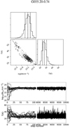 |
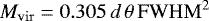
Fig. 1 Three upper panels: corner plot for the source G035.20-0.74 of the two parameters
|


4.1.2 Spectral energy distribution fitting
The SEDs have been modeled as a modified black body with
 (1)
(1)
where Fν is the observed flux density at the frequency ν, Bν (Tdust) is the Planck function at the dust temperature Tdust, τν is the optical depth at the frequency ν and Ω is the source solid angle, given by Ω = π∕(4ln2) θ2. The optical depth can be written as:
 (2)
(2)
where  is the mean molecular weight, mH is the mass of the hydrogen atom,
  is the molecular hydrogen column density,
  is the dust opacity at the reference frequency ν0, and β is the spectral index. We have adopted a value of 2.8 for
  (Kauffmann et al. 2008), a dust opacity of 0.8 cm2 g−1 at ν0 = 230 GHz (Ossenkopf & Henning 1994), assuming a gas-to-dust ratio of 100, and a value of β = 2.
The SEDs have been fitted using a Monte Carlo Markov chain (MCMC) algorithm that minimizes the χ2 modeling the observed data with Eq. (1), with 20 chains and a number of iterations equal to 10000. The two free parameters, Tdust and  , have been constrained inside a range of 6−60 K and 1020−1025 cm−2 respectively. These ranges are consistent with mean values from Elia et al. (2017). A first run with a lower number of iterations has been done with larger boundaries, and all the preliminary fit values have been found within the ranges given above, validating the choice of the ranges. The results of the best fit are given in Table 4: Tdust ranges from 9 to 36 K, while the values of
  cover about two orders of magnitude from 3 × 10²¹ to 7 × 1023 cm−2. Figure 1 shows the path of the random walkers for the two free parameters and the corner plot with the results of the fit, for the source G035.20-0.74 as an example. The SED and the best fit model are shown in Fig. 2. The orange area shows the results of the models using values for Tdust and
  within the uncertainties from the best-fit values.
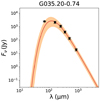 |
Fig. 2 SED of the source G035.20-0.74. The red line is the best fit to the SED, obtained using the parameters
|

4.1.3 Mass and luminosity estimates
Two important physical parameters are the mass and the luminosity of the sources. The mass was derived using the molecular hydrogen column density derived in Sect. 4.1.2:
 (3)
(3)
where d is the distanceof the source.
The total flux F in the far-IR band,for the 69 objects for which we have been able to construct the SEDs, has been calculated as the discrete integral of the best fit model of the SED between 10 and 3 mm:
 (4)
(4)
For sources for which the ratio between the observed flux at 70 μm and the flux at 70 μm of the best-fit model of the SED is larger than 10% (~80% of the sources), we added the flux excess to the total flux from Eq. (4). The flux excess has been calculated assuming that for λ < λp, where λp is the wavelength at which Fλ peaks (in our sample always larger than 70 μm), the flux of the source at any λ is given by the value derived from the linear interpolation between the flux at λp and the flux at 70 μm, or between the flux at 70 μm and the flux at 10 μm, for 10 μm < λ < 70 μm. The luminosity has been derived from the total flux using:
 (5)
(5)
The modified blackbody emission of dust modeled is expected to underestimate the flux densities for wavelengths shorter than 70 μm for evolved sources suchas HMPOs and UC HII regions (see SEDs in König et al. 2017). We have calculated a part of the flux excess from the values of flux at 70 μm. However, what we included is not the totality of the flux excess. Thus the luminosities of HMPOs and UC HIIs are likely underestimated, because it is not possible to derive from the data collected here the part of flux excess at shorter wavelengths. For the cold and least evolved sources, HMSCs, the emission at shorter wavelengths is expected to be negligible and not to show excess from the observed SED. Table 5 lists the luminosity L and the ratio L∕M. The ratio L∕M, which is a distance independent parameter, is an indicator of evolution since its value increases as a source evolves: in the first evolutionaryphase more gas is converted into stars during the star formation process and the embedded source(s) becomes more luminous, thus the mass of the clump remains nearly constant while its luminosity increases, while in the second phase the young stellar object (YSO) is already on the zero-age main sequence (ZAMS) and starts to clean-up its surroundings, leading to a decrease of the mass of the clump (Molinari et al. 2008, 2016, 2019; Giannetti et al. 2017b; Elia et al. 2017, 2021; König et al. 2017). Since the most evolved sources in our sample are UC HII regions, the expected L∕M increase in our sample would be related to the first accretion phase.
Mass, luminosity, and L∕M ratio.
4.2 CH3CN analysis
The spectra at 3 mm of the CH3CN(5K−4K) transitions toward the 85 sources presented in this work have been analyzed with the SLIM (Spectral Line Identification and Modeling) tool within the MADCUBA package7 (Martín et al. 2019). At least one of the five K-components has been detected toward 73 targets in the sample (85% of the total sample), reported in Column 3 of Table 6, while in Col. 4 the K components for which the signal-to-noise ratio S/N is larger than three are given. Before analyzing the spectra, a first order baseline has been removed, determining the best fit of the baseline from free-channels around the lines.
To obtain the parameters of the molecular emission ( , Tex, FWHM and VLSR), we used the AUTOFIT tool of MADCUBA-SLIM, which finds the best agreement between the observed spectra and the predicted LTE model, taking into account also the optical depth. We performed the fit assuming that all the transitions are populated with the same Tex and that the emission fills the beam, therefore the column densities of methyl cyanide have been computed inside a diameter of 26.6′′, the IRAM 30 m telescope beam (θb). We calculated the corrected column density,
  , using the beam-dilution factor
  . The single excitation temperature assumption is justified by the high densities of high-mass star-forming regions, comparable or larger than the values of the critical densities, ncrit, for CH3CN(5K−4K) transitions which are in the range 1−3 × 105 cm−3 for T in the range 20−140 K8.
The results of the fit are given in Table 6, together with the CH3CN abundance  . The spectraare given in Appendix A. For the source G31.41+0.31, the fit does not converge. This could be the combined result of high opacity at the center of this HMC, together with the presence of a temperature gradient (Beltrán et al. 2005, 2018; Cesaroni et al. 2011), that makes a single Tex fit impossible.
For the sources in which only the component K = 0 has been detected, the fit has been performed including also higher transitions, since their upper limits can give constraints during the fitting procedure. Moreover, even if not detected above 3σ level, in several cases the K = 1 transition is close to the 2σ level (or above) and its inclusion in the fit has allowed the determination of Tex. Only for I22134-B and 20332+4124 M1 we had to fix Tex to 25 and 44 K, respectively. These two values have been chosen from a visual inspection of the spectra, varying Tex and  to search for a couple of parameter where the K = 0 was visually well reproduced and the simulated higher K components (not detected) with intensity below or comparable with the noise.
For the sources for which at least the transitions K = 0, 1, and 2 were detected, we calculated a rotational diagram using the specific tool of MADCUBA-SLIM. The values of Tkin derived from the rotational diagram are consistent within the errors with the values of Tex from AUTOFIT, except for two sources: 18454-0136 M1 and 19095+0930. For 18454-0136 M1 Tex = 35 ± 6 K while Tkin = 59 ± 3 K. However, including in the rotational diagram the upper limit of the K = 3 transition, the value of Tkin decreases to 22 K. For 19095+0930, Tex = 57 ± 4 K while Tkin = 74 ± 12 K. The inclusion of the upper limits of the K = 4 transition does not change the results of the rotational diagram, thus this is the only source for which we have found a clear discrepancy between Tkin and Tex. The Tex derived from the best agreement between the synthetic spectrum of all the (5K −4K) transitions and the observed spectrum is thus a reliable estimate of the Tkin of the sources. The goodness of the fit and the agreement between Tex and Tkin indicates noneed for a hotter component arising from a smaller region, when analyzing the CH3CN(5K−4K) transitions. Giannetti et al. (2017b) also found that the (5K −4K) and (6K −5K) transitions are well reproduced by a single temperature fit, while to model the higher energy (19K−18K) transitions a second hotter component is needed.
Results of the fit of CH3CN(5K−4K).
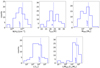 |
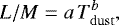
Fig. 3 Histograms of the distribution of H2 column density, dust temperature, mass (upper panel from left to right), luminosity, and luminosity-to-mass ratio (lower panel from left to right), respectively, in the sample. The dotted vertical lines indicate the mean value of the distribution. Data are given in Tables 4 and 5. |
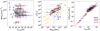 |
Fig. 4 Left: distribution of the sources of the sample in the plane N(H2) − Tdust. Middle: distribution of the sources of the sample in the plane L − MSED). Gray tracks are the evolutionary tracks from Molinari et al. (2008), while orange dashed lines indicate L∕M = 1, 10, and 100 L⊙∕M⊙. Right: plot of the evolutionary tracers L∕M as a function of Tdust and power-law relation best fit to the data given in orange. The legend for the classification color-code is given in the right panel. Sources that have not been classified yet are plotted in black. |
4.3 Virial mass and virial parameter
To discuss the gravitational stability of the targets we have also derived the virial masses, Mvir, that for a spherical system are defined as (MacLaren et al. 1988):
 (6)
(6)
where σ is the three-dimensional velocity dispersion, R is the radius of the object, and k1 = (5 − 2n)∕(3 − n) assuming a density profile ρ ∝ r−n. Assuming n = 2 (i.e., ρ ∝ r−2) and a gaussian velocity distribution, Eq. (6) can be written as:
 (7)
(7)
in units M⊙, where θ is the angular dimension of the sources in arcsec, and FWHM is the linewidth in km s−1 (see MacLaren et al. 1988). We then derived the virial parameter α = Mvir∕MSED (Kauffmann et al. 2013), reported in Table 6.
5 Discussion
5.1 Physical properties derived from the SEDs
Figure 3 shows the histograms of the distribution of molecular hydrogen column density, dust temperature, mass, luminosity, and luminosity-to-mass ratio for the sample. The values of  cover two orders of magnitude from 3 × 10²¹ to 7 × 1023 cm−2, while Tdust ranges from 9 to 36 K. These ranges are consistent with those found in works with similar or larger samples (Elia et al. 2017; König et al. 2017). The luminosity of the sources spans over four orders of magnitude, from ~ 30 to 300 000 L⊙, while the mass ranges from ~30 and 8000 M⊙. Lastly, the luminosity-to-mass ratio L∕M covers more than three orders of magnitude from 6 × 10⁻² to 3 × 10² L⊙∕M⊙. The sources are located at different distances, from 0.7 to 13 kpc, and the linear scales traced range from ~ 0.1 and ~ 1.4 pc, with a mean value of ~ 0.45 pc, and with only nine sources (~13%) with diameters below 0.2 pc. Thus, the considered structures are likely associated with clumps, and only in a few cases with cores, which are smaller and denser structures embedded inside a clump. This explains the broad ranges obtained for the masses and the luminosities.
Figure 4 shows the distribution of the sample in the space  and L − MSED, with different colors indicating the sources already classified (see last panel for the legenda). The plot of
  vs. Tdust does not highlight any trend between the two quantities and with evolutionary stage. The lack of any particular trend between surface density and dust temperature has been seen before on a sample of ~ 105 sources in the work of Elia et al. (2017) for Tdust > 20 K. On the last panel (right) we show the relation between L∕M and Tdust; the plot highlights a clear correlation between the two physical quantities. The best fit to the data, assuming a power-law:
 (8)
(8)
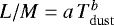
is given by a = (2.9 ± 1.5) × 10−7 L⊙∕M⊙ K−b and b = (5.8 ± 0.2), and is represented by the orange line in Fig. 4. The red line in Fig. 4 is the theoretical prediction for an optically thin modified blackbody (Elia & Pezzuto 2016):
 (9)
(9)
where kB is the Boltzmann constant, h is the Planck constant, c is the speed of light, Γ is the Euler gamma function, and ζ is the Riemann zeta function. With our assumption on β and the dust opacity coefficient it can be written as:
 (10)
(10)
consistent with the best fit.
The positive correlation seen is consistent with L∕M tracing the evolution of the sources, as already discussed in previous studies (Molinari et al. 2008; Urquhart et al. 2014, 2018; Giannetti et al. 2017b; Elia et al. 2017, 2021). These studies indicated that massive young stellar objects (YSO) – HMPO, UC HII or more evolved sources that have already dissipated their envelope – are characterized by a L∕M ratio between ~1 L⊙∕M⊙ and ~100 L⊙∕M⊙. Lower values, L∕M < 1 L⊙∕M⊙, are associated with earliest stages in which no star formation is yet present or is in a very early evolutionary stage. Alternatively, these cores could only contain embedded low-mass YSOs. However, Elia et al. (2017) showed that prestellar objects have a narrower distribution in L∕M, compared to protostellar sources that are widely distributed, and highlighted the presence of a statistically significant overlap of the distributions in the two classes. It is thus possible to find HMPOs with values lower than ~ 1 L⊙∕M⊙, or HMSCs with higher values. Molinari et al. (2019) confirmed that the L∕M ratio is a good tracer of the evolutionary stage of star formation, running a grid of 20 million synthetic protocluster models. From Fig. 9 in Molinari et al. (2019), the models in which at least one young stellar object (YSO) is a zero age main sequence (ZAMS) star, are in good agreement with L∕M > 1 L⊙∕M⊙, confirming that L∕M < 1 L⊙∕M⊙ indicates the earliest stage of star formation.
The position of the HMSC sources in the plot L vs. MSED and L∕M vs. Tdust is consistent with values of L∕M ≲ 1 L⊙∕M⊙, with the exception of the sources I00117-MM2, I20293-WC and I22134-B. Among these, the high L∕M value in I00117-MM2 can be explained in terms of contamination of the fluxes used to build the SED by the nearby source I00117-MM1 (HMPO), which is only ~ 16′′ apart. A similar contamination can be present in the following couples of sources due to their proximity: AFGL5142-MM and AFGL5142-EC (~ 11′′), I19035-VLA1 and 19035+0641M1 (~ 8′′), 19410+2336M1 and 19410+2336 (~ 9′′), I22134-VLA1 and I22134-G (~ 21′′), and 23033+5951 and 23033+5951M1 (~ 11′′). However, these are compact and centrally peaked sources, therefore the molecular emission inside the telescope beam would be dominated by the main source, and not by the nearby companions. These sources also constitute the ~ 44% of Subsample I, thus a large fraction of the classified subsample. For these reasons we decided not exclude them from the analysis. From the sources in Subsample I, UC HII regions are associated with larger values of the luminosity-to-mass ratio than HMPO (with only one exception), thus giving another confirmation of the clear growth of L∕M with evolution. The majority of the sources of the Subsample II (black dots) have values of L∕M mostly larger than 10 L⊙∕M⊙. Therefore it is likely that these sources are in more evolved evolutionary phases, being either HMPOs or UCHII regions. A small number of sources in Subsample II are well studied sources in evolved stages, like for instance the HMCs G31.41+0.31 and G24.78+0.08 (e.g., Cesaroni et al. 2011; Beltrán et al. 2011b), for which we have derived values of ~ 20−25 L⊙∕M⊙. However from this figure and from the analysis in Sect. 5.2, five unclassified sources of Subsample II show values of L∕M closer to thevalues of HMSCs and are likely to be themselves starless cores or very early HMPOs. An accurate classification of the sources in the Subsample II, obtained from the fluxes of these sources in the mid-IR and at cm wavelengths, will be presented in a following paper.
 |
Fig. 5 Histograms of the distribution of column density of CH3CN (left panel), excitation temperature Tex
(middle panel), and abundance |

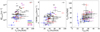 |
Fig. 6 Left: plot of the column densities of CH3CN as a functionof the excitation temperature Tex. Middle: plot of the FWHM of CH3CN as a functionof the excitation temperature Tex. Right: plot of the excitation temperature Tex of methyl cyanide vs. dust temperature Tdust. The gray line indicates Tdust = Tex. |
5.2 Physical properties derived from CH3CN
We detected at least one of the CH3CN(5K−4K) K-transitions in each of the ~86% of the sources observed in the sample. The histogram of the distributions of the column density  , excitation temperatureTex, and abundance
  are given in Fig. 5. The column densities cover a range of three orders of magnitude, from ~ 2 × 1011 cm−2 to ~ 2 × 1014 cm−2, while the abundances are in the range ~7 × 10⁻¹²−9 × 10⁻¹⁰.
Figure 6 shows that both column density and line-width (FWHM) of CH3CN increase with excitation temperature, Tex. This implies that warmer sources have a higher degree of turbulence, as expected, and also higher values of the column density. Moreover, Fig. 6 shows the correlation between Tdust and Tex of CH3CN. This also highlights that Tex is always larger (or in a few cases equal) than Tdust.
The virial parameter α = Mvir∕MSED vs. MSED is plotted in Fig. 7. From its definition, the virial parameter can be written as α = a(2 Ekin)∕Epot (Bertoldi & McKee 1992), where Ekin is the kinetic energy, Epot is the gravitational potential energy, and a is a geometrical factor that depends on the symmetry and gas density distribution of the considered “cloud”. For non-magnetized gas, the critical value of α, αcrit, which is the value that separates gravitationally stable (α > αcrit) from unstable objects (α < αcrit), is 2 ± 1 (Kauffmann et al. 2013). This implies that sources with α > 2 may expand due to their kinetic motion, while sources with α <2 are gravitationally bound. In our sample, 72% of the sources9 show values α < 2, while only 28% show values above 2. However, the latter sources may be confined by the pressure of the surrounding gas. On the other hand, the presence of magnetic fields can give support to unstable objects, leading to a lower value of αcrit which depends on the strength of the magnetic field itself (see e.g., Bertoldi & McKee 1992 and Kauffmann et al. 2013).
The mean values of  10, Tex, and
  for the total sample are given in Table 7. From the mean values within the evolutionary classes of Subsample I, we can see that there is a clear positive trend of
  with evolutionary stage, with the highest difference of about one order of magnitude among HMSCs and more evolved sources. In the case of
  , there is a clear increase from the earliest stage of star-formation to the more evolved stages, with at least one order of magnitude of difference between HMSC and HMSCw or more evolved sources, similarly to what was found for the column density. However, there is not a clear distinction in abundance between HMPOs and UC HII regions. An evolution of mean abundances with star-formation evolutionary phase has been also found by Coletta et al. (2020) for other COMs, such as methyl formate, dimethyl ether, and ethyl cyanide analyzing 39 sources belonging to our sample, with the clearest increasing trends found for methyl formate and dimethyl ether.
The mean values of  for different evolutionary phases found by previous single-dish studies are given in Table 8. The comparison is not straightforward considering the different assumptions, the different transitions observed, and the intrinsic differences between sources that can have different values of
  . Hung et al. (2019) estimate the highest values of column densities, on average two orders of magnitude above the values found in our sample toward the most evolved sources. However, from Table 5 in their paper we can see that they corrected for filling factor η ~ 10−3−10−4 in most cases, while in the sources presented in this paper η ~ 7 × 10⁻²−1. For the comparison with the work of Giannetti et al. (2017b) we took the data from the VizieR On-line Data Catalog: J/A+A/603/A33 (Giannetti et al. 2017a). We considered only the cool component of methyl cyanide, that is able to reproduce the emission of the CH3CN(5K-4K) and (6K -5K) transitions, while a hotter component is needed for the higher energy transitions (19K-18K) in their study. The column density is corrected for η, ranging from 1 to ~10−2. In Table 8 we list the mean values over the different evolutionary phases. These show an increase with evolutionary stage, confirming what we found with our study. The column densities of methyl cyanide toward the sample of Giannetti et al. (2017b) have been previously studied by Sabatini et al. (2021) – considering both the cool and hot component – showing an upward trend with evolution of the mean column densities in the different evolutionary phases, and in agreement with the predictions of the chemical network presented in their work. However, the mean estimate of
  for HMSCs in this work is one order of magnitude below the mean values found by Giannetti et al. (2017b) for 70 μm-weak sources. This may not be a real discrepancy if HMSCs in our work are on average less evolved than the selected 70 μm-weak sources in Giannetti et al. (2017b). The mean values found by Rosero et al. (2013) for HMPOs are consistent with our estimates within a factor ~2.5, while the values found by Araya et al. (2005) in UC HII regions are on average a factor ~ 10 larger than what we found in this paper. The mean values from Purcell et al. (2006) are consistent with our estimates, with the biggest difference of a factor ~3 found among the values for cores with no maser emission and radio-quiet, and our HMSCs. Potapov et al. (2016) found a column density of methyl cyanide of ~6 × 1011 cm−2, in a cold dense core in TMC-1C. This is consistent with our estimates in HMSCs within a factor ~ 2.
Methyl cyanide emission has been detected in all three evolutionary classes, from HMSCs to UC HII regions. This confirms what was found by Olmi et al. (1996b) and Giannetti et al. (2017b), who showed that CH3CN is not a tracer of evolved objects only: transitions associated with (relatively) low energies are detected also in very young objects, and thus are mostly tracers of dense gas.
In addition to the trend seen in Table 7 for the mean values of  , in Fig. 8 we can see that the abundances of CH3CN increase with both indicators of evolution, Tdust, and the ratio L∕M. The two plots show a clear correlation, although with some dispersion. From the Subsample I, we can see that the less evolved sources, HMSCs possibly not contaminated – i.e., HMSCs with L∕M < 1 L⊙∕M⊙ and Tdust < 15 K – have abundances of
  that do not exceed the value of 2.0 × 10⁻¹¹, and that only HMSCs are found below 4.0 × 10⁻¹¹. For HMPOs and UC HII regions there is not a clear separation in the values of abundances. Moreover, we can see that five sources of the Subsample II show low values of
  , close to that of HMSCs in the Subsample I. These sources also have low values of L∕M and Tdust. These sources are G014.99−0.67, 18310−0825M3, 18445−0222M3, G015.02−0.62, and 18454−0136M1. The first three sources have L∕M between 2.0 and 4.0 L⊙∕M⊙ and Tdust of 16 K, while G015.02−0.62 and 18454−0136M1 have L∕M ~ 12−15 L⊙∕M⊙ and Tdust ~ 20 K. However, G015.02−0.62 and G014.99−0.67 are not detected at 70 μm, while the other three have flux densities consistent with those observed toward the HMSCs of Subsample I. These sources have masses in the range ~ 1−8 × 10² M⊙ and are located within ~ 5 kpc from the Sun, but the distance ambiguity is not resolved for 18310−0825M3, 18445−0222M3, and 18454−0136M1, therefore these three sources may be located further away. However, both L∕M and Tdust are distance-independent and the assumption of the far distance would lead to larger values of mass. We note that there is no ambiguity in the distance of G015.02−0.62 and G014.99−0.67 (~ 2 kpc) and these sources have masses >100 M⊙, therefore the fact that they are not detected at 70 μm is not attributable to far and/or not massive enough sources. For this reason we conclude that these sources are likely in very early phases, possibly being HMSCs or early HMPOs, and that
  can be a very useful and practical tool to identify high-mass sources in the earliest stages of star formation, when a multiwavelength analysis to derive Tdust or L∕M is not possible. We give as conservative upper limit for HMSCs
 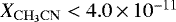 , while the region between
  (gray area in Fig. 8) is likely populated by HMSCs or very early HMPOs.
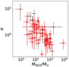 |
Fig. 7 Plot of α = Mvir∕MSED as a function of MSED. The black dashed line represents α = 2. |
Mean values of column density corrected for beam-dilution, abundance, and excitation temperature of CH3CN in the TOPGöt sample.
Mean values of column density and excitation temperature of CH3CN for different evolutionary classes in literature works.
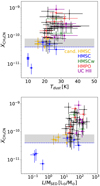 |
Fig. 8 Distribution of the abundances of CH3CN as a function of the two indicators of evolution Tdust (top panel) and L∕M (bottom panel). The yellow points represent the five sources of Subsample II identified as early evolutionary stage, candidates HMSCs or very early HMPOs. The blue dashed line indicates the conservative threshold for abundances of methyl cyanide of 4 × 10⁻¹¹ (only HMSCs), while the gray area indicates the abundance range in which the sources are most likely HMSCs or very early HMPOs. |
5.3 CH3CN nondetections
Of the 85 sources observed in CH3CN(5K − 4K), we have 12 nondetections: one HMSC (G034−F2(MM7)) and eleven sources of the Subsample II, thus unclassified sources likely HMPOs or UC HII regions (see Sect. 5.1). To understand if there is a physical limit in the detection of CH3CN, we have plotted the column densities of H2 against the dust temperature in Fig. 9, highlighting in gray the nine sources that show no detection of methyl cyanide and for which we have been able to construct the SED. G034−F2(MM7) is the source that in the total sample shows the lowest temperature, being possibly the youngest object of the TOPGöt sample. It is thus possible that in this case not enough methyl cyanide has been formed in this source in order to be detected. Other three sources (18290−0924M2, G042.03+0.19 and G042.70−0.15) show very low values of  (~ 3.5 × 1021 cm−2): also in these cases the nondetections may be due to a limit in sensitivity. The remaining five cases are not of clear interpretation, in fact other sources with similar
  show the emission of CH3CN. Thus, in these five cases it is possible that the nondetections are related to a chemical differentiation of these sources with respect to the others.
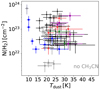 |
Fig. 9 Distribution of sources in the plane |

6 Conclusions
In this workwe have presented the TOPGöt sample that arises from the combination of two separate subsamples (Subsample I and Subsample II) of high-mass star-forming regions containing 86 sources. These sources have been observed with the IRAM 30 m telescope in several spectral windows, allowing studies of different classes of molecules. In this first paper we have constructed the SEDs, derived the physical properties of the sample, and analyzed the emission of CH3CN(5K-4K) using MADCUBA. We summarize below the main results of this study:
-
We have built the SED for 69 of the 86 total sources in the sample (80%). The derived Tdust and
 are between 9 and 36 K
and ~3 × 10²¹−7 × 1023 cm−2, respectively.
are between 9 and 36 K
and ~3 × 10²¹−7 × 1023 cm−2, respectively. -
The luminosity spans over four orders of magnitude in the sample, from ~30 to 3 × 10⁵ L⊙, while masses vary between ~30 to 8 × 10³ M⊙. The luminosity-to-mass ratio L∕M covers three orders of magnitude from 6 × 10⁻² to 3 × 10² L⊙∕M⊙.
-
The luminosity-to-mass ratio L∕M, a robust evolutionary indicator as seen in previous studies (Molinari et al. 2008, 2016, 2019; Urquhart et al. 2014; Giannetti et al. 2017b), shows a tight positive correlation with Tdust, well reproduced by a power-law (
 ) as expected from Elia & Pezzuto (2016). The parameters of the best-fit are a = (2.9 ± 1.5) × 10−7 L⊙∕M⊙ K−b
and b = (5.8 ± 0.2).
) as expected from Elia & Pezzuto (2016). The parameters of the best-fit are a = (2.9 ± 1.5) × 10−7 L⊙∕M⊙ K−b
and b = (5.8 ± 0.2). -
At least one of the CH3CN(5K-4K) K-components has been detected toward 73 sources (85%), with 12 nondetections and one source not observed. The emission of methyl cyanide has been detected toward all the evolutionary stages, and the values of column density show a good agreement with previous studies, taking into account the difference in beam-filling factors and observations beams.
-
The mean values of the column density of methyl cyanide show a clear positive trend with evolutionary stages. This behavior is also confirmed by the data of Giannetti et al. (2017b) and their analysis by Sabatini et al. (2021). However, the mean values of observed abundances show an increase of one order of magnitude among HMSCs and more evolved sources, but no clear distinction between HMPOs and UC HII regions in the TOPGöt sample. An increase in abundances with evolutionary stages has been found by Coletta et al. (2020) for other COMS such as methyl formate, dimethyl ether and ethyl cyanide, and it is a powerful tool to infer the evolutionary stage of a source without performing a multiwavelength analysis.
-
From the comparison of values of
 in already classified sources of the Subsample I, we found five good candidates of HMSCs or very early HMPOs in Subsample II. The robustness of the
  value as a tracer of early evolutionary stages is confirmed by the low values of L∕M,
Tdust, and flux densities at 70 μm for these sources. This is an example of the importance of tools such as molecular evolutionary indicators. In particular, methyl cyanide is a widespread molecule which emits bright transitions, thus this result can be easily applied to identify sources in early stages.
value as a tracer of early evolutionary stages is confirmed by the low values of L∕M,
Tdust, and flux densities at 70 μm for these sources. This is an example of the importance of tools such as molecular evolutionary indicators. In particular, methyl cyanide is a widespread molecule which emits bright transitions, thus this result can be easily applied to identify sources in early stages. -
We propose a conservative upper limit of
 of 4.0 × 10⁻¹¹
for clearly HMSCs and a range between 4.0 × 10⁻¹¹
and 7.0 × 10⁻¹¹
in which we could find HMSCs and possibly very early HMPOs.
of 4.0 × 10⁻¹¹
for clearly HMSCs and a range between 4.0 × 10⁻¹¹
and 7.0 × 10⁻¹¹
in which we could find HMSCs and possibly very early HMPOs.
In conclusion, from the analysis of CH3CN(5K-4K), we have found that low excitation transitions of methyl cyanide have been detected toward all the evolutionary stages of high-mass star-forming regions and that it is possible to use the abundance of methyl cyanide as a tracer of very early stages of the star-formation process.
Acknowledgements
The authors thank the anonymous referee for his/her comments, that improved this work. This work is based on observations carried out with the IRAM 30 m telescope. IRAM is supported by INSU/CNRS (France), MPG (Germany) and IGN (Spain). C.M. acknowledges support from the Italian Ministero dell’Istruzione, Università e Ricerca through the grant Progetti Premiali 2012 – iALMA (CUP C52I13000140001) and from the European Research Council (ERC) under the European Union’s Horizon 2020 program, through the ECOGAL Synergy grant (grantID 855130). L.C. acknowledges financial support through Spanish grant PID2019-105552RB-C41 (MINECO/MCIU/AEI/FEDER) and from the Spanish State Research Agency (AEI) through the Unidad de Excelencia “María de Maeztu”-Centro de Astrobiología (CSIC-INTA) project No. MDM-2017-0737. V.M.R. acknowledges support from the Comunidad de Madrid through the Atracción de Talento Investigador Modalidad 1 (contratación de doctores con experiencia)Grant (COOL: Cosmic Origins Of Life; 2019-T1/TIC-15379). This work was partly supported by the Italian Ministero dell Istruzione, Università e Ricerca through the grant Progetti Premiali 2012 – iALMA (CUP C52I13000140001), by the Deutsche Forschungs-gemeinschaft (DFG, German Research Foundation) – Ref no. FOR 2634/1 TE 1024/1-1, and by the DFG cluster of excellence Origins (www.origins-cluster.de). This project has received funding from the European Union’s Horizon 2020 research and innovation programme under the Marie Sklodowska-Curie grant agreement No 823823 (DUSTBUSTERS) and from the European Research Council (ERC) via the ERC Synergy Grant ECOGAL (grant 855130). We acknowledge support from the Gothenburg Centre of Advanced Studies in Science and Technology through the program “Origins of habitable planets” in 2016, when the TopGöt project was initiated.
Appendix A Methyl cyanide spectra
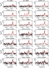 |
Fig. A.1 Spectra of CH3CN(5K-4K) for the sources for which at least one transition has been detected. The red line is the synthetic spectrum obtained by the best fit within MADCUBA. For G31.41+0.31, the synthetic spectrum is not reported since the fit does not converge. VLSR of sources G014.99-0.67 and 18445-0222M3 during observations mildly differ from the correct value. VLSR has been corrected after observations, and given in Table 3. |
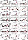 |
Fig. A.2 Continued |
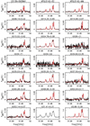 |
Fig. A.3 Continued |
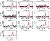 |
Fig. A.4 Continued |
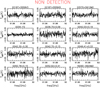 |
Fig. A.5 Spectra of CH3CN(5K-4K) for the sources for which no transition has been detected. |
References
- Agúndez, M., Cernicharo, J., Quintana-Lacaci, G., et al. 2015, ApJ, 814, 143 [NASA ADS] [CrossRef] [Google Scholar]
- Araya, E., Hofner, P., Kurtz, S., Bronfman, L., & DeDeo, S. 2005, ApJS, 157, 279 [NASA ADS] [CrossRef] [Google Scholar]
- Arce, H. G., Santiago-García, J., Jørgensen, J. K., Tafalla, M., & Bachiller, R. 2008, ApJ, 681, L21 [NASA ADS] [CrossRef] [Google Scholar]
- Balog, Z., Müller, T., Nielbock, M., et al. 2014, Exp. Astron., 37, 129 [NASA ADS] [CrossRef] [EDP Sciences] [Google Scholar]
- Belloche, A., Garrod, R. T., Müller, H. S. P., et al. 2019, A&A, 628, A10 [NASA ADS] [CrossRef] [EDP Sciences] [Google Scholar]
- Beltrán, M. T., Cesaroni, R., Neri, R., et al. 2004, ApJ, 601, L187 [NASA ADS] [CrossRef] [Google Scholar]
- Beltrán, M. T., Cesaroni, R., Neri, R., et al. 2005, A&A, 435, 901 [NASA ADS] [CrossRef] [EDP Sciences] [Google Scholar]
- Beltrán, M. T., Cesaroni, R., Neri, R., & Codella, C. 2011a, A&A, 525, A151 [NASA ADS] [CrossRef] [EDP Sciences] [Google Scholar]
- Beltrán, M. T., Cesaroni, R., Zhang, Q., et al. 2011b, A&A, 532, A91 [CrossRef] [EDP Sciences] [Google Scholar]
- Beltrán, M. T., Cesaroni, R., Rivilla, V. M., et al. 2018, A&A, 615, A141 [NASA ADS] [CrossRef] [EDP Sciences] [Google Scholar]
- Bendo, G. J., Griffin, M. J., Bock, J. J., et al. 2013, MNRAS, 433, 3062 [NASA ADS] [CrossRef] [Google Scholar]
- Bergman, P., & Hjalmarson, A. 1989, Methyl Cyanide (CH3CN) in Molecular Cloud Cores, eds. G. Winnewisser, & J. T. Armstrong (Berlin: Springer), 331, 124 [Google Scholar]
- Bergner, J. B., Guzmán, V. G., Öberg, K. I., Loomis, R. A., & Pegues, J. 2018, ApJ, 857, 69 [Google Scholar]
- Bertoldi, F., & McKee, C. F. 1992, ApJ, 395, 140 [NASA ADS] [CrossRef] [Google Scholar]
- Beuther, H., Walsh, A., Schilke, P., et al. 2002, A&A, 390, 289 [NASA ADS] [CrossRef] [EDP Sciences] [Google Scholar]
- Beuther, H., Churchwell, E. B., McKee, C. F., & Tan, J. C. 2007, in Protostars and Planets V, eds. B. Reipurth, D. Jewitt, & K. Keil (Tucson: University of Arizona Press), 165 [Google Scholar]
- Bonnell, I. A., & Bate, M. R. 2006, MNRAS, 370, 488 [NASA ADS] [CrossRef] [Google Scholar]
- Busquet, G., Palau, A., Estalella, R., et al. 2010, A&A, 517, L6 [NASA ADS] [CrossRef] [EDP Sciences] [Google Scholar]
- Cesaroni, R., Felli, M., Jenness, T., et al. 1999, A&A, 345, 949 [NASA ADS] [Google Scholar]
- Cesaroni, R., Beltrán, M. T., Zhang, Q., Beuther, H., & Fallscheer, C. 2011, A&A, 533, A73 [NASA ADS] [CrossRef] [EDP Sciences] [Google Scholar]
- Churchwell, E., Walmsley, C. M., & Wood, D. O. S. 1992, A&A, 253, 541 [NASA ADS] [Google Scholar]
- Codella, C., Benedettini, M., Beltrán, M. T., et al. 2009, A&A, 507, L25 [NASA ADS] [CrossRef] [EDP Sciences] [Google Scholar]
- Coletta, A., Fontani, F., Rivilla, V. M., et al. 2020, A&A, 641, A54 [CrossRef] [EDP Sciences] [Google Scholar]
- Colzi, L., Fontani, F., Caselli, P., et al. 2018a, A&A, 609, A129 [NASA ADS] [CrossRef] [EDP Sciences] [Google Scholar]
- Colzi, L., Fontani, F., Rivilla, V. M., et al. 2018b, MNRAS, 478, 3693 [NASA ADS] [CrossRef] [Google Scholar]
- Colzi, L., Fontani, F., Caselli, P., et al. 2019, MNRAS, 485, 5543 [CrossRef] [Google Scholar]
- Compiègne, M., Flagey, N., Noriega-Crespo, A., et al. 2010, ApJ, 724, L44 [NASA ADS] [CrossRef] [Google Scholar]
- Csengeri, T., Urquhart, J. S., Schuller, F., et al. 2014, A&A, 565, A75 [NASA ADS] [CrossRef] [EDP Sciences] [Google Scholar]
- Cyganowski, C. J., Whitney, B. A., Holden, E., et al. 2008, AJ, 136, 2391 [NASA ADS] [CrossRef] [Google Scholar]
- Di Francesco, J., Johnstone, D., Kirk, H., MacKenzie, T., & Ledwosinska, E. 2008, ApJS, 175, 277 [NASA ADS] [CrossRef] [Google Scholar]
- Elia, D., & Pezzuto, S. 2016, MNRAS, 461, 1328 [NASA ADS] [CrossRef] [Google Scholar]
- Elia, D., Molinari, S., Schisano, E., et al. 2017, MNRAS, 471, 100 [NASA ADS] [CrossRef] [Google Scholar]
- Elia, D., Merello, M., Molinari, S., et al. 2021, MNRAS, 504, 2742 [NASA ADS] [CrossRef] [Google Scholar]
- Faúndez, S., Bronfman, L., Garay, G., et al. 2004, A&A, 426, 97 [NASA ADS] [CrossRef] [EDP Sciences] [Google Scholar]
- Fontani, F., Palau, A., Caselli, P., et al. 2011, A&A, 529, L7 [NASA ADS] [CrossRef] [EDP Sciences] [Google Scholar]
- Fontani, F., Busquet, G., Palau, A., et al. 2015a, A&A, 575, A87 [NASA ADS] [CrossRef] [EDP Sciences] [Google Scholar]
- Fontani, F., Caselli, P., Palau, A., Bizzocchi, L., & Ceccarelli, C. 2015b, ApJ, 808, L46 [NASA ADS] [CrossRef] [Google Scholar]
- Fontani, F., Vagnoli, A., Padovani, M., et al. 2018, MNRAS, 481, 79 [CrossRef] [Google Scholar]
- Furuya, R. S., Cesaroni, R., Takahashi, S., et al. 2008, ApJ, 673, 363 [NASA ADS] [CrossRef] [Google Scholar]
- Giannetti, A., Leurini, S., Wyrowski, F., et al. 2017a, Vizie R Online Data Catalog: J/A+A/603/A33 [Google Scholar]
- Giannetti, A., Leurini, S., Wyrowski, F., et al. 2017b, A&A, 603, A33 [NASA ADS] [CrossRef] [EDP Sciences] [Google Scholar]
- Green, S. 1986, ApJ, 309, 331 [NASA ADS] [CrossRef] [Google Scholar]
- Hung, T., Liu,S.-Y., Su, Y.-N., et al. 2019, ApJ, 872, 61 [NASA ADS] [CrossRef] [Google Scholar]
- Immer, K., Li,J., Quiroga-Nuñez, L. H., et al. 2019, A&A, 632, A123 [CrossRef] [EDP Sciences] [Google Scholar]
- Johnston, K. G., Robitaille, T. P., Beuther, H., et al. 2015, ApJ, 813, L19 [NASA ADS] [CrossRef] [Google Scholar]
- Kalenskii, S. V., Promislov, V. G., Alakoz, A., Winnberg, A. V., & Johansson, L. E. B. 2000, A&A, 354, 1036 [NASA ADS] [Google Scholar]
- Kauffmann, J., Bertoldi, F., Bourke, T. L., Evans, N. J., I., & Lee, C. W. 2008, A&A, 487, 993 [NASA ADS] [CrossRef] [EDP Sciences] [Google Scholar]
- Kauffmann, J., Pillai, T., & Goldsmith, P. F. 2013, ApJ, 779, 185 [NASA ADS] [CrossRef] [Google Scholar]
- Keto, E. 2007, ApJ, 666, 976 [NASA ADS] [CrossRef] [Google Scholar]
- König, C., Urquhart, J. S., Csengeri, T., et al. 2017, A&A, 599, A139 [NASA ADS] [CrossRef] [EDP Sciences] [Google Scholar]
- Krumholz, M. R., Klein, R. I., McKee, C. F., Offner, S. S. R., & Cunningham, A. J. 2009, Science, 323, 754 [NASA ADS] [CrossRef] [PubMed] [Google Scholar]
- Loomis, R. A., Cleeves, L. I., Öberg, K. I., et al. 2018, ApJ, 859, 131 [NASA ADS] [CrossRef] [Google Scholar]
- MacLaren, I., Richardson, K. M., & Wolfendale, A. W. 1988, ApJ, 333, 821 [NASA ADS] [CrossRef] [Google Scholar]
- Martín, S., Martín-Pintado, J., Blanco-Sánchez, C., et al. 2019, A&A, 631, A159 [NASA ADS] [CrossRef] [EDP Sciences] [Google Scholar]
- McKee, C. F., & Tan, J. C. 2003, ApJ, 585, 850 [Google Scholar]
- Minh, Y. C., Liu, H. B., & Galvań-Madrid, R. 2016, ApJ, 824, 99 [NASA ADS] [CrossRef] [Google Scholar]
- Mininni, C., Fontani, F., Rivilla, V. M., et al. 2018, MNRAS, 476, L39 [NASA ADS] [CrossRef] [Google Scholar]
- Molinari, S., Brand, J., Cesaroni, R., & Palla, F. 1996, A&A, 308, 573 [NASA ADS] [Google Scholar]
- Molinari, S., Pezzuto, S., Cesaroni, R., et al. 2008, A&A, 481, 345 [NASA ADS] [CrossRef] [EDP Sciences] [Google Scholar]
- Molinari, S., Swinyard, B., Bally, J., et al. 2010, A&A, 518, L100 [NASA ADS] [CrossRef] [EDP Sciences] [Google Scholar]
- Molinari, S., Schisano, E., Faustini, F., et al. 2011, A&A, 530, A133 [NASA ADS] [CrossRef] [EDP Sciences] [Google Scholar]
- Molinari, S., Schisano, E., Elia, D., et al. 2016, A&A, 591, A149 [NASA ADS] [CrossRef] [EDP Sciences] [Google Scholar]
- Molinari, S., Baldeschi, A., Robitaille, T. P., et al. 2019, MNRAS, 486, 4508 [NASA ADS] [CrossRef] [Google Scholar]
- Motte, F., Bontemps, S., & Louvet, F. 2018, ARA&A, 56, 41 [NASA ADS] [CrossRef] [Google Scholar]
- Mueller, K. E., Shirley, Y. L., Evans, Neal J., I., & Jacobson, H. R. 2002, ApJS, 143, 469 [Google Scholar]
- Müller, H. S. P., Thorwirth, S., Roth, D. A., & Winnewisser, G. 2001, A&A, 370, L49 [NASA ADS] [CrossRef] [EDP Sciences] [Google Scholar]
- Müller, H. S. P., Schlöder, F., Stutzki, J., & Winnewisser, G. 2005, J. Mol. Struc., 742, 215 [Google Scholar]
- Müller, H. S. P., Brown, L. R., Drouin, B. J., et al. 2015, J. Mol. Spectr., 312, 22 [NASA ADS] [CrossRef] [Google Scholar]
- Öberg, K. I., Guzmán, V. V., Furuya, K., et al. 2015, Nature, 520, 198 [Google Scholar]
- Olmi, L., Cesaroni, R., & Walmsley, C. M. 1993, A&A, 276, 489 [NASA ADS] [Google Scholar]
- Olmi, L., Cesaroni, R., & Walmsley, C. M. 1996a, A&A, 307, 599 [NASA ADS] [Google Scholar]
- Olmi, L., Cesaroni, R., Neri, R., & Walmsley, C. M. 1996b, A&A, 315, 565 [NASA ADS] [Google Scholar]
- Ossenkopf, V.,& Henning, T. 1994, A&A, 291, 943 [Google Scholar]
- Pankonin, V., Churchwell, E., Watson, C., & Bieging, J. H. 2001, ApJ, 558, 194 [NASA ADS] [CrossRef] [Google Scholar]
- Potapov, A., Sánchez-Monge, Á., Schilke, P., et al. 2016, A&A, 594, A117 [NASA ADS] [CrossRef] [EDP Sciences] [Google Scholar]
- Purcell, C. R., Balasubramanyam, R., Burton, M. G., et al. 2006, MNRAS, 367, 553 [NASA ADS] [CrossRef] [Google Scholar]
- Remijan, A., Sutton, E. C., Snyder, L. E., et al. 2004, ApJ, 606, 917 [NASA ADS] [CrossRef] [Google Scholar]
- Rivilla, V. M., Colzi, L., Fontani, F., et al. 2020, MNRAS, 496, 1990 [NASA ADS] [CrossRef] [Google Scholar]
- Rosero, V., Hofner, P., Kurtz, S., Bieging, J., & Araya, E. D. 2013, ApJS, 207, 12 [Google Scholar]
- Sabatini, G., Bovino, S., Giannetti, A., et al. 2021, A&A, 652, A71 [NASA ADS] [CrossRef] [EDP Sciences] [Google Scholar]
- Sánchez-Monge, Á., Palau, A., Estalella, R., Beltrán, M. T., & Girart, J. M. 2008, A&A, 485, 497 [NASA ADS] [CrossRef] [EDP Sciences] [Google Scholar]
- Sánchez-Monge, Á., Pandian, J. D., & Kurtz, S. 2011, ApJ, 739, L9 [NASA ADS] [CrossRef] [Google Scholar]
- Schuller, F., Menten, K. M., Contreras, Y., et al. 2009, A&A, 504, 415 [NASA ADS] [CrossRef] [EDP Sciences] [Google Scholar]
- Solomon, P. M., Jefferts, K. B., Penzias, A. A., & Wilson, R. W. 1971, ApJ, 168, L107 [NASA ADS] [CrossRef] [Google Scholar]
- Spezzano, S., Caselli, P., Bizzocchi, L., Giuliano, B. M., & Lattanzi, V. 2017, A&A, 606, A82 [NASA ADS] [CrossRef] [EDP Sciences] [Google Scholar]
- Sridharan, T. K., Beuther, H., Schilke, P., Menten, K. M., & Wyrowski, F. 2002, ApJ, 566, 931 [Google Scholar]
- Tafalla, M., Myers, P. C., Caselli, P., & Walmsley, C. M. 2004, A&A, 416, 191 [NASA ADS] [CrossRef] [EDP Sciences] [Google Scholar]
- Tan, J. C., Kong, S., Zhang, Y., et al. 2016, ApJ, 821, L3 [NASA ADS] [CrossRef] [Google Scholar]
- Traficante, A., Calzoletti, L., Veneziani, M., et al. 2011, MNRAS, 416, 2932 [Google Scholar]
- Urquhart, J. S., Moore, T. J. T., Csengeri, T., et al. 2014, MNRAS, 443, 1555 [Google Scholar]
- Urquhart, J. S., König, C., Giannetti, A., et al. 2018, MNRAS, 473, 1059 [NASA ADS] [CrossRef] [Google Scholar]
- Vastel, C., Bottinelli, S., Caux, E., Glorian, J. M., & Boiziot, M. 2015, in SF2A-2015: Proceedings of the Annual meeting of the French Society of Astronomy and Astrophysics, 313 [Google Scholar]
- Zahorecz, S., Jimenez-Serra, I., Wang, K., et al. 2016, A&A, 591, A105 [NASA ADS] [CrossRef] [EDP Sciences] [Google Scholar]
- Zhang, Q., Ho, P. T. P., & Ohashi, N. 1998, ApJ, 494, 636 [NASA ADS] [CrossRef] [Google Scholar]
- Zhang, Q., Hunter, T. R., Sridharan, T. K., & Ho, P. T. P. 2002, ApJ, 566, 982 [NASA ADS] [CrossRef] [Google Scholar]
- Zhang, B., Zheng, X. W., Reid, M. J., et al. 2009, ApJ, 693, 419 [Google Scholar]
The name of the project originates from the city in which it had been firstly ideated, Göthenburg, as part of the GoCAS program “Origins of Habitable Planets” that was held in the Gothenburg Centre for Advanced Studies in Science and Technology from May 2, 2016 to June 10, 2016: https://www.chalmers.se/en/centres/GoCAS/Events/ Origins-of-Habitable-Planets/Pages/default.aspx
For a complete documentation see https://cdms.astro.uni-koeln.de/cgi-bin/cdmsinfo?file=e041505.cat
Madrid Data Cube Analysis (MADCUBA) is a software developed in the Center of Astrobiology (Madrid) to visualize and analyze data cubes and single spectra: https://cab.inta-csic.es/madcuba/
The collisional coefficients have been taken from the CASSIS (Vastel et al. 2015) Collision Database: http://cassis.irap.omp.eu/download/collisions/files/CH3CN-H2-cdms.dat. The entry is based on Green (1986).
For 14 sources detected in CH3CN we do not have the emission maps to build the SED, and thus an estimate of
θ. Therefore, for these sources we have used the values of column density not corrected for the beam-dilution to calculate the mean value. For these sources we do not have an estimate of  and thus they were not included in the determination of the mean value of abundance.
All Tables
Sources coordinates, heliocentric distances, line-of-sight velocities, and evolutionary phases (e.p.).
Mean values of column density corrected for beam-dilution, abundance, and excitation temperature of CH3CN in the TOPGöt sample.
Mean values of column density and excitation temperature of CH3CN for different evolutionary classes in literature works.
All Figures
|
Fig. 1 Three upper panels: corner plot for the source G035.20-0.74 of the two parameters
|
| In the text | |
|
Fig. 2 SED of the source G035.20-0.74. The red line is the best fit to the SED, obtained using the parameters
|
| In the text | |
|
Fig. 3 Histograms of the distribution of H2 column density, dust temperature, mass (upper panel from left to right), luminosity, and luminosity-to-mass ratio (lower panel from left to right), respectively, in the sample. The dotted vertical lines indicate the mean value of the distribution. Data are given in Tables 4 and 5. |
| In the text | |
|
Fig. 4 Left: distribution of the sources of the sample in the plane N(H2) − Tdust. Middle: distribution of the sources of the sample in the plane L − MSED). Gray tracks are the evolutionary tracks from Molinari et al. (2008), while orange dashed lines indicate L∕M = 1, 10, and 100 L⊙∕M⊙. Right: plot of the evolutionary tracers L∕M as a function of Tdust and power-law relation best fit to the data given in orange. The legend for the classification color-code is given in the right panel. Sources that have not been classified yet are plotted in black. |
| In the text | |
|
Fig. 5 Histograms of the distribution of column density of CH3CN (left panel), excitation temperature Tex
(middle panel), and abundance |
| In the text | |
|
Fig. 6 Left: plot of the column densities of CH3CN as a functionof the excitation temperature Tex. Middle: plot of the FWHM of CH3CN as a functionof the excitation temperature Tex. Right: plot of the excitation temperature Tex of methyl cyanide vs. dust temperature Tdust. The gray line indicates Tdust = Tex. |
| In the text | |
|
Fig. 7 Plot of α = Mvir∕MSED as a function of MSED. The black dashed line represents α = 2. |
| In the text | |
|
Fig. 8 Distribution of the abundances of CH3CN as a function of the two indicators of evolution Tdust (top panel) and L∕M (bottom panel). The yellow points represent the five sources of Subsample II identified as early evolutionary stage, candidates HMSCs or very early HMPOs. The blue dashed line indicates the conservative threshold for abundances of methyl cyanide of 4 × 10⁻¹¹ (only HMSCs), while the gray area indicates the abundance range in which the sources are most likely HMSCs or very early HMPOs. |
| In the text | |
|
Fig. 9 Distribution of sources in the plane |
| In the text | |
|
Fig. A.1 Spectra of CH3CN(5K-4K) for the sources for which at least one transition has been detected. The red line is the synthetic spectrum obtained by the best fit within MADCUBA. For G31.41+0.31, the synthetic spectrum is not reported since the fit does not converge. VLSR of sources G014.99-0.67 and 18445-0222M3 during observations mildly differ from the correct value. VLSR has been corrected after observations, and given in Table 3. |
| In the text | |
|
Fig. A.2 Continued |
| In the text | |
|
Fig. A.3 Continued |
| In the text | |
|
Fig. A.4 Continued |
| In the text | |
|
Fig. A.5 Spectra of CH3CN(5K-4K) for the sources for which no transition has been detected. |
| In the text | |
Current usage metrics show cumulative count of Article Views (full-text article views including HTML views, PDF and ePub downloads, according to the available data) and Abstracts Views on Vision4Press platform.
Data correspond to usage on the plateform after 2015. The current usage metrics is available 48-96 hours after online publication and is updated daily on week days.
Initial download of the metrics may take a while.