| Issue |
A&A
Volume 648, April 2021
|
|
|---|---|---|
| Article Number | A84 | |
| Number of page(s) | 11 | |
| Section | Atomic, molecular, and nuclear data | |
| DOI | https://doi.org/10.1051/0004-6361/202040023 | |
| Published online | 15 April 2021 | |
Binding energies and sticking coefficients of H2 on crystalline and amorphous CO ice
1
Institute for Theoretical Chemistry, University of Stuttgart,
Pfaffenwaldring 55,
70569
Stuttgart,
Germany
e-mail: This email address is being protected from spambots. You need JavaScript enabled to view it.
2
Institute of Low Temperature Science, Hokkaido University, N19W8, Kita-ku, Sapporo,
Hokkaido,
Japan
Received:
30
November
2020
Accepted:
7
March
2021
Abstract
Context. Molecular hydrogen (H2) is the most abundant interstellar molecule and plays an important role in the chemistry and physics of the interstellar medium. The interaction of H2 with interstellar ices is relevant for several processes (e.g., nuclear spin conversion and chemical reactions on the surface of the ice). To model surface processes, quantities such as binding energies and sticking coefficients are required.
Aims. We provide sticking coefficients and binding energies for the H2/CO system. These data are absent in the literature so far and could help modelers and experimentalists to draw conclusions on the H2/CO interaction in cold molecular clouds.
Methods. Ab initio molecular dynamics simulations, in combination with neural network potentials, were employed in our simulations. Atomistic neural networks were trained against density functional theory calculations on model systems. We sampled a wide range of H2 internal energies and three surface temperatures.
Results. Our results show that the binding energy for the H2/CO system is low on average, − 157 K for amorphous CO and −266 K for crystalline CO. This carries several implications for the rest of the work. H2 binding to crystalline CO is stronger by 109 K than to amorphous CO, while amorphous CO shows a wider H2 binding energy distribution. Sticking coefficients are never unity and vary strongly with surface temperature, but less so with ice phase, with values between 0.95 and 0.17. With the values of this study, between 17 and 25% of a beam of H2 molecules at room temperature would stick to the surface, depending on the temperature of the surface and the ice phase. Residence times vary by several orders of magnitude between crystalline and amorphous CO, with the latter showing residence times on the order of seconds at 5 K. H2 may diffuse before desorption in amorphous ices, which might help to accommodate it in deeper binding sites.
Conclusions. Based on our results, a significant fraction of H2 molecules will stick on CO ice under experimental conditions, even more so under the harsh conditions of prestellar cores. However, with the low H2–CO binding energies, residence times of H2 on CO ice before desorption are too short to consider a significant population of H2 molecules on pure CO ices. Diffusion is possible in a time window before desorption, which might help accommodate H2 on deeper binding sites, which would increase residence times on the surface.
Key words: ISM: molecules / molecular data / astrochemistry / methods: numerical
© ESO 2021
1 Introduction
Interstellar H2 is the most abundant gas-phase molecule in cold, interstellar environments. The formation of H2 in these environments requires a third body to dissipate the H + H → H2 reaction exothermicity (Wakelam et al. 2017). The third body in these astronomical environments is assumed to be an interstellar dust grain. Dust grains consist of a refractory nucleus, whose chemical composition is in general amorphous carbon or silicates, and an envelope of soft ices that accrete on top of the refractory core under the conditions of cold environments (e.g., molecular clouds). In addition, interstellar ices present multiple (hypothetically stratified) phases (Boogert et al. 2015). The primary molecule in interstellar ices is H2O, and it additionally acts as the main constituent of the so-called polar phase of the ice (Boogert et al. 2015), which is formed primarily at T > 20 K. At harsher conditions, T < 20 K, with a lower H/CO ratio and overall higher particle density (n > 104 cm−3), apolar molecules can accrete as well, on top of the polar phase. CO ice is known to be the main molecule in the apolar phase.
Even though H2 is mainly formed in the solid phase, the nondissipated heat of formation and the weak nature of the H2 binding to molecular solids will return H2 to the media. H2 can eventually collide again with dust grains in different evolution states, stick to the surface, diffuse, and desorb again. In water-ice surfaces, this process has been studied experimentally (Govers et al. 1980; Matar et al. 2010; He et al. 2016a) and by our recent simulations (Molpeceres & Kästner 2020).
Quantifying the amount of H2 that returns to the solid phase is important for several reasons. H2 is an important factor in gas-phase ion-molecule reactions (Wakelam et al. 2012), and its prevalence in the solid phase can have a direct effect on molecular abundances in prestellar cores. In addition, the ortho–para ratio (OPR), as a measure of the relation between the two possible nuclear spin states of the H2 molecule, is a very useful proxy to track physical and chemical processes in cold environments (see, e.g., Bron et al. 2016 and references therein). The statistical OPR from H + H recombination is 3, while the equilibrium value at lowtemperature is close to zero. When values other than the statistical value are obtained in cold environments (Maret & Bergin 2007; Pagani et al. 2009; Troscompt et al. 2009), alternative scenarios for ortho-para spin conversion are needed. These include conversion via gas-phase reactions with ionic species and conversion on dust grains. H2 abstraction reactions from other species are much less exothermic than H + H recombination and could lead to significant changes in the OPR (Meisner et al. 2017; Lamberts & Kästner 2017; Oba et al. 2018; Álvarez-Barcia et al. 2018). The conversion mechanism on dust grains has been postulated to be the interaction with inhomogeneities of the surface (Fukutani & Sugimoto 2013), but it is not completely understood. Regardless of the conversion mechanism, it has been shown that in amorphous solid water (ASW), conversion can take place on laboratory timescales, 6.4 × 10² to 4.1 × 10³ s (Watanabe et al. 2010; Ueta et al. 2016).
Quantities governing the fraction of molecules that return to the gas phase after a collision with an ice surface are sticking coefficients (ST) and residence times. The sticking coefficient represents the fraction of molecules that remains adsorbed after a collision. Residence times quantify the time that a particular adsorbate stays on a surface after adsorption. Both quantities are affected by the binding energy of an adsorbate with a surface. While sticking coefficients and binding energies of H2 on ASW are available in the literature (Govers et al. 1980; Matar et al. 2010; He et al. 2016a,b; Molpeceres & Kästner 2020), values for other substrates in an astronomical context are rarer. Acharyya (2014) presented the study of H2 sticking on an olivine surface, for example. It has recently been suggested that the sticking coefficients and residence times for the H2 /CO system must vary strongly in the temperature range of 8–20 K (Chuang et al. 2018).
With this paper, we study the interaction of H2 with CO ice computationally, employing ab initio molecular dynamics simulations and providing binding energies and sticking coefficients for this pair. The dominant ice phase of CO at cryogenic temperatures is difficult to assert because the range of conditions where amorphous CO is present is small (Kouchi 1990), but recent studies indicate that crystalline CO is the dominant phase under astrophysical conditions (Kouchi et al. 2021). As models for the ice, we therefore employed both crystalline and amorphous analogs. Theoretical attempts to study surface processes on top of the CO ice range from applications of Monte Carlo simulations of hydrogen atom reactivity (Fuchs et al. 2009), classical molecular dynamics simulation of CO photodesorption (Van Hemert et al. 2015), kinetic Monte Carlo simulations of CO mobility on top of H2O (Karssemeijer et al. 2014; Lauck et al. 2015), or ab initio molecular dynamics simulations of radical-radical recombination on top of CO clusters (Lamberts et al. 2019).
Our methods provide a new level of accuracy in the simulation of adsorption processes. Extensive sampling in ab initio molecular dynamics simulations is prohibitively expensive, even at a moderate level of theory. To overcome this limitation, we have employed state of the art atomistic neural network potentials based on Gaussian moments as molecular descriptors (Zaverkin & Kästner 2020).
The paper is organized as follows. First, we start with a description of our theoretical framework, outlining the generation of our training set, the training procedure, the surface construction, and the collision dynamics description that is required to evaluate thesticking coefficients. Second, we discuss our results, with binding energies, sticking coefficients, and H2 /CO residence times. Finally, we set our findings into perspective of the astrophysical picture, and we summarize the main points of our study.
2 Theoretical methods
The evaluation of the quantities presented in this work requires a precise description of the atomic forces and energies in the structure. We used machine-learned potentials (MLP) for this task. The Gaussian moment neural network (GM-NN) developed in our group was used. The description of the method (Zaverkin & Kästner 2020) and its application to astrophysical systems (Molpeceres et al. 2020) have been discussed previously. In this work, we only present the particularities of the H2 /CO system.
2.1 Generation of the training set
To construct the neural-network potential, a sufficiently representative training set at a suitable underlying level of theory is required. We employed density functional theory calculations (DFT) to the generate the training set. For the exchange and correlation functional and basis set combination, we used BHLYP-D4 (Becke 1993; Caldeweyher et al. 2019) and def2-TZVP (Weigend & Ahlrichs 2005), respectively. BHLYP-D4 was chosen from a range of exchange and correlation functionals that were compared to more exact CCSD(T)-F12/cc-pVTZ-F12 energies on both the CO–CO and the CO–H2 dimer. Details on this benchmark can be found in Appendix A. All electronic structure calculations were carried out with the Turbomole code (version 7.4) (Balasubramani et al. 2020). The procedure for the extraction of points is similar to the one in our previous work (Molpeceres et al. 2020). We used a sampling strategy based on a quick exploration of the potential energy surface (PES) in model systems (small clusters) at a computationally cheap level of theory, from which we extracted snapshots to be refined at the theory level mentioned above. For this work, a quick exploration of the PES was made using the recent GFN-FF force-field (Spicher & Grimme 2020) and molecular dynamics simulations. All energy and force solvers used during the generation of the training set were integrated within the ChemShell (Sherwood et al. 2003; Metz et al. 2014) suite of programs, allowing an on-the-fly application of our protocol.
The training set was constructed with two objectives in mind. First, having an accurate description of the CO–CO interaction, and second, an equally good representation of the H2 /CO interaction. For the first objective, we ran molecular dynamics simulations in the NVT ensemble of pre-optimized (GFN-FF level) CO clusters of two different sizes (30 and 40 CO molecules), with an integration time step of 1 fs and a Berendsen thermostat. The simulations were run at 20 and 1000 K. The first is intended to explore stable structures around the equilibrium positions of the cluster, whereas the second has the goal of sampling high-energy situations that should be avoided by the neural network. To ensure a minimum structural integrity of the cluster at high temperatures, a spherical (radius of 20 Bohr), harmonic boundary potential was incorporated into the simulation. We generated the initial clusters by random placement of CO molecules using the Packmol code (Martinez et al. 2009). The second part of the training set was developed by running collision dynamics (NVE, time step 0.5 fs) between a H2 molecule and a 10 CO cluster (generated in the same way as above). Initial velocities for the cluster atoms were extracted from a random Maxwell–Boltzmann distribution at 100 K. H2 molecules were placed at random points distributed spherically around the cluster and were provided with an initial energy of ~50 K (50 trajectories) and ~300 K (200 trajectories). Snapshots were extracted only when H2 molecules were <6 Å away from any other atom of the cluster, according to the cutoff radius employed in our machine learned potentials (see below). The reason behind these seemingly harsh conditions for the collision dynamics is to provide enough kinetic energy to both CO and H2 to extensively sample the configurational space of the system. All the parameters for the training set generation simulations and the frequency ofsnapshot extraction are gathered in Table 1.
Structures, temperatures (T, in K), and time interval between snapshots extraction for refinement (f, in fs) and total number of structures (N) included in the training set to construct the neural network potential.
2.2 Training of the neural network potential
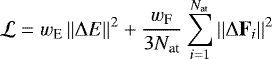
To construct the MLP, we employed the GM-NN model, which uses molecular descriptors based on Gaussian moments (GMs; Zaverkin & Kästner 2020). The environment of each atom is described within a cutoff sphere by the molecular descriptor. To fit the high-dimensional potential energy surface, we trained the neural network on total energies and atomic forces. We employed a cutoff radius of 6 Å to account for long-range interactions between H2 and CO molecules. The loss function
 (1)
(1)
was minimized to train the neural network. Nat correspondsto the total number of atoms in a specific structure, and ΔE and ΔFi are the absolute deviations between prediction and reference data for energies and forces, respectively. wE and wF are weights that modulate the contribution of the energy and force to the loss function. They were set to 1 au and 100 au Å2, respectively. The neural network was selected to contain two hidden layers. The first layer comprises 256 nodes and the second 128. Initial weights and biases of the neural network were initialized randomly and subsequently optimized using the AMSGrad optimizer (Reddi et al. 2019) with 32 structures per minibatch. Training of the models was carried out using the Tensorflow library (Abadi et al. 2015) for 5000 training epochs using an NVIDIA Tesla V100 GPU. For validation, 18% of the training set was reserved, and the remaining 82% was included in the training. Assessment of the MLP quality was carried out similarly to our previous work (Molpeceres et al. 2020) by comparing outputs from three independently trained models, finding deviations of < ~1 kcal mol−1 Å−1 between them in the relevant regions of the surface. Slightly higher errors of ~ 2–3 kcal mol−1 Å−1 were sometimes found in the fixed atoms regions due to the energetically unfavorable arrangements during placement (see below). While this error is still acceptable, these regions were never sampled in the binding energy calculations or in the sticking dynamics. The agreement in the binding energies of H2 on CO between our MLP potential and the underlying DFT method was assessed by calculating the interaction profile of an optimized cluster of 10 CO molecules and one H2, with a rigid potential energy surface scan. The results of this validation are shown in Appendix A.
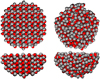 |
Fig. 1 Side and top views of the relaxed carbon monoxide ice surface models employed in our simulations. On the left we show the crystalline surface, and on the right the amorphous surface. |
2.3 Creation of the surface models
To study the surface properties, we created two different CO ice models. First, a crystalline bulk of α-CO crystal (P213 space group, Vegard 1930) was cut in the crystallographic (110) direction, using the slab generator tool in Avogadro (Hanwell et al. 2012). The (110) CO direction is the most stable crystallographic orientation (Fuchs et al. 2009). We used a perfectly ordered CO ice model, while in reality, C and O of each molecule can be exchanged randomly. From this initial slab containing 2480 CO molecules, we extracted a hemispheric selection of 488 CO molecules. The outermost 172 CO molecules were kept fixed to provide a boundary for the ice. After an initial optimization using the MLP within the atomic simulation environment (ASE; Hjorth Larsen et al. 2017), the hemisphere generated this way has a density of 1.07 g cm−3, in good agreement with the experimental value for the α-CO crystal (1.05 g cm−3 at 6 K) (Krupskii et al. 1973). Second, we randomly placed 477 CO molecules in a hemisphere to create the amorphous CO ice using Packmol (Martinez et al. 2009). We fixed here 183 CO molecules of the external layer to again provide a hard boundary tothe ice. This initial hemisphere was relaxed using our neural network potential. Figure 1 depicts the final shape of the optimized hemispheres. Our models are large clusters, and therefore, they are not periodic.
The relaxed ices were then raised to the simulation temperatures following two different procedures, one for the crystalline ice and a different procedure for the amorphous ice. In the case of the crystalline procedure, ices were briefly heated to 5, 10, and 20 K for 10 ps from the relaxed structure. For the amorphous procedure, we heated the ice at 75 K for 100 ps, extracting 20 equispaced snapshots during the warming phase. Each of these snapshots was suddenly quenched to5, 10, and 20 K for 10 ps to generate 20 uncorrelated amorphous ice structures at each temperature. During collision dynamics, these ices were selected randomly to ensure statistical sampling of different collision points.
2.4 Collision dynamics setup
The calculation of sticking coefficients requires the evaluation of collision trajectories of H2 with our icearchetypes. The sampling strategy for studying the collisions follows the same protocol as our previous works (Molpeceres & Kästner 2020; Molpeceres et al. 2020). Very briefly, targeting a collision point located in the center of the hemisphere plus a random lateral displacement in the x and y directions, we calculate the center of mass position of the H2 molecule and its velocity vector, satisfying three initial conditions. These conditions are the initial kinetic energy of the molecule (E), the polar angle of incidence (θ), and the azimuthal angle of incidence (ϕ). The initial incoming energy is an input parameter that we here varied between 12 and 350 K. It is relevant to mention that all the initial kinetic energy of the molecule is translational, with no initial rotational or vibrational energy. The polar angles of incidence were sampled equidistantly for values in between 0° and 60°. These angles were defined to the surface normal. The azimuthal angle was sampled randomly between 0° and 360°. The initial z component of the center of mass of the H2 molecule was set to be at ~8 Å. Finally, the initial orientation of the H2 molecule was randomized. Molecular dynamics simulations were carried out in the NVE ensemble with the velocity-Verlet algorithm, using an integration time step of 0.5 fs and a maximum simulation time of 10 ps. The trajectories were propagated using the MD implementation within ASE (Hjorth Larsen et al. 2017). At the end of every trajectory, if any of the H atoms in the H2 molecule was at a distance >6 Å, we considered that trajectory as bounced, and in the opposite case, as stuck. The threshold of 6 Å also implies an energetic criterion to the determination of a sticking event. Above 6 Å (our training cutoff radius), our potential is smoothly truncated and H2 behaves like a free particle without interaction with the surface, therefore representing definitive bouncing. From the ratio of stuck to total number of trajectories at a particular incoming energy, we extracted the sticking probability P(E) with an associated error. The error was extracted from a binomial distribution of events at a confidence level of 95% using a Jeffreys interval and calculated using the Statsmodels mathematical library (Seabold & Perktold 2010).
3 Results
3.1 Binding energies of H2 on CO
To sample binding sites, we minimized H2/CO configurations spanning a quadratic selection of 400 Å2 of the surface at lateral intervals of 1 Å. The H2 molecule centers of mass (COM) were placed at a minimum distance of 1.5 Å over the surface in the crystalline sample. For the amorphous ice, and given the roughness of the surface, we varied the position of the H2 COM to ensure a minimum distance of 2.5 Å to any other atom in the surface. Binding energies were obtained as the difference between these energies (Eclose) and the energy of H2 far from the surface (Efar), Ebin= Eclose − Efar. We employed the optimization routines within ASE for the energy and force minimization of the structures (Hjorth Larsen et al. 2017).
The distribution of binding energies is depicted in Fig. 2. In the case of the crystalline structure, we observe a prominent bin at ~−250 K corresponding to binding in mostly hollow and bridge sites in the structure, whereas lower binding energy values correspond to top binding sites (see Fig. 3). Because of boundary effects, our model deviates from perfect crystallinity, which slightly broadens the distribution. Overall, the best compromise for an average of the binding energy in the crystalline ice is to employ the median of the binding energy distribution. The weakest bound molecules are expected to diffuse into the stronger-binding hollow sites. The median for this distribution is −266 K, which is the value we employ during the remaining paper.
Binding in the case of amorphous CO is different. The surface contains many different binding sites, which is the expected behavior of an amorphous surface. In this case, we can extract a representative binding energy from the mean value of the distribution, corresponding to −157 K with a standard deviation of 75 K.
These binding energies represent unmistakably weakly physisorbed states. Binding energies are slightly higher in the case of the crystalline structure, but are very low nonetheless. These values do not contain the vibrational zeropoint energy (ZPE). An accurate estimation of the ZPE is difficult in these cases because of the anharmonicity of the H–CO low-frequency vibrations.
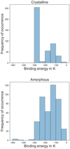 |
Fig. 2 Distribution of binding energies for the H2/CO system. In the upper panel for a crystalline surface, and in the lower panel for an amorphous one. |
 |
Fig. 3 Adsorption sites for the H2 molecule on top of crystalline CO. Left panel: top, middle panel: bridge. Right panel: hollow. |
Summary of the sticking probabilities (P(E)) obtained in this work as a function of the ice phase, particle incoming energy (E), and surface temperature (TS).
3.2 Sticking coefficients
To calculate the sticking coefficients, we carried out collision dynamics as described in Sect. 2.4. For this task, we must distinguish between three different temperatures. First, the surface temperature (TS). Second, the incoming energy (in Kelvin) (E), representing the kinetic energy given to the H2 in a particular set of trajectories at a given TS. Third and last, thegas temperature (Tg), corresponding to an assumed thermalized gas obeying a Maxwell–Boltzmann distribution of velocities. The gas temperature is employed inthe integration of thermal sticking coefficients (see below). We carried out collision dynamics for E = 12, 35, 58, 93, 116, 174, 232, 290, and 348 K for TS = 5, 10, and 20 K. For every E we sampled 16 θ and 12 ϕ angles. This makes a total of 192 trajectories per E. Crystalline and amorphous samples were considered equally. In total, we sampled 10,368 different trajectories.
Sticking probabilities (P(E)) calculated as the ratio of sticking versus total number of events for a particular E/TS pair are represented in Fig. 4 and Table 2. We observe the expected behavior for this type of weakly physisorbed species (Molpeceres & Kästner 2020; Molpeceres et al. 2020). For low E, we observe a plateau of predominantly sticking events up to E ~ 90 K. Second, a steep decay of the sticking probabilities for intermediate temperatures (100 K < E < 250 K) until we reach a majority of bouncing events with little changes between the last two energies (290 and 340 K). At low energies it is possible that a trajectory is labeled as bounced when it fulfills the bounce criteria while having lower energy than the interaction energy at 6 Å (−5 K at the CCSD(T)-F12 level of theory, see Appendix A). The effect of such errors is expected to remain small, given that the respective sticking probabilities are rather high (with values of about 0.85 and 0.93). Moreover, such a deviation would be minimized in the thermal averaging procedure, see below.
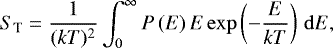
Thermal integration of the distribution of sticking probabilities allowed us to obtain the thermal sticking coefficients, which are more useful for comparison with experiments and are of direct use for modelers. This thermal integration was carried out with the following expression (Buch & Zhang 1991):
 (2)
(2)
with k being Boltzmann’s constant. We estimated the error bar in ST as describedpreviously (Molpeceres et al. 2020). Boundary conditions for the integration were set as P(0) = 1 and P(∞) = 0. The results of this integration can be found in Fig. 5 and Table 3. While we employed H2 kinetic energies only down to 12 K, the thermal integration was made starting at lower temperatures for TS = 5, 10 K. The results between 12 and 0 K are interpolated between our sampled values at 12 K and the P(0) = 1 boundary condition. Sticking coefficients are in general higher for crystalline samples, as expected from its higher binding energy (Sect. 3.1). The sticking coefficient is never unity in our calculations, even for TS as low as 5 K. At Tg = 300 K, sticking coefficients are still about 0.2, indicating that under normal experimental conditions, it should be possible to observe H2 sticking on cold substrates. The effect of surface temperature is noticeable, considering the small range of surface temperatures considered in our experiments (only 15 K). At low Tg, the decrease of the sticking coefficient as a function of the surface temperature is ~ 20%. Changes for TS with values of 5 and 10 K are less noticeable at low Tg. As in previous studies, sticking coefficients presented here represent instantaneous sticking coefficients after a collision. We did not take desorption events at times above our simulation time (10 ps) into account. Our simulations are thus decoupled from spontaneous desorption. Therefore H2 can have mobility on the ice surface before it is desorbed to the media (see next section). Our results confirm the hypothesis presented by Chuang et al. (2018), who assumed a strong dependence of the sticking coefficient of H2 on the CO surface temperature in the range between 8 and 20 K. While the estimate is true, here we show that the main factor affecting sticking coefficient is the adsorbate internal energy.
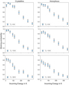 |
Fig. 4 Sticking probabilities P(E) of the H2/CO system at different surface temperatures. Left panel: crystalline sample. Right panel: amorphous sample. |
Summary of the sticking coefficients (ST) obtained in this work as a function of the ice phase, gas temperature (Tg), and surface temperature (TS).
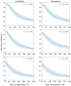 |
Fig. 5 Integrated sticking coefficients ST of the H2/CO system at different surface temperatures. Left panel: crystalline sample. Right panel: amorphous sample. All curves start at Tg = TS. |
3.3 Residence times
As the last part of our study, we have estimated the spontaneous desorption half-lifetime employing transition state theory. The half-lifetime is calculated as
 (3)
(3)
where kd is the characteristic rate constant for desorption. kd is calculatedas
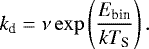 (4)
(4)
In Eq. (4), Ebin is our binding energy (calculated in Sect. 3.1) and ν is the attempt frequency for a desorption event. ν corresponds to the vibration perpendicular to the surface in the z direction. To obtain this frequency, we ran long collision dynamics (25 ps) for unambiguous sticking trajectories (E = 12 K, TS = 10 K, and θ = 0°) both for crystalline and amorphous structures. We obtained the variation on the H2 center of mass z position and its associated maxima from the trajectories. Attempt frequencies were estimated as the inverse of time differences between two maxima (see Fig. 6). In Fig. 6, we represent the value of the z coordinate of the H2 center of mass and not the minimum distance to any other CO molecule in the system. Only maxima after 5 ps (after a number of initial bounces) were considered. Finally, our employed attempt frequency is obtained as the averaged value of all the considered values.
For crystalline ice, νcrys = 1∕0.314 ps = 3.18 ps−1. In the case of amorphous ice, this value yields νamor = 1∕0.257 ps = 3.89 ps−1. Results of the application of Eq. (3) are presented in Table 4. These residence times are very short in all cases, except for the crystalline with TS = 5 K case. These results agree with the experimental findings by Chuang et al. (2018), who concluded that a significant fraction of H2 not present in the bulk after deposition returned to the gas phase. Residence times are longer for crystalline ice than for amorphous ice by several orders of magnitude, given the higher binding energy on this surface. As discussed in the next section, the results presented here refer to quite flat surfaces without macroscopic or mesoscopic defects. Such defects can affect the distribution of binding sites under experimental conditions. Overall, spontaneous desorption in our models occurs on short timescales. Desorption half-lifetime is a good estimator of residence times, given our low binding energies. According to our results, H2 is not likely tobind to CO surfaces on astronomically relevant timescales.
In the case of amorphous ice at lower temperatures, a more in-depth analysis of residence times can be made on the basis of a whole distribution of binding sites. Distributions of residence times, calculated at four different surface temperatures (5, 8, 10, and 20 K), are shown in Fig. 7. From the graph, it is clear that in a significant fraction of the binding sites (about 40% at 5 K) H2 is able to remain adsorbed more than 1 × 10³ s. At slightly higher temperatures such as 8 or 10 K, the fraction of binding sites able to accommodate H2 for longer times is reduced to 1–2%. However, on a real ice, the number of binding sites (deep and narrow) will be much higher, and H2 could diffuse in the μs to ms time frame to deep binding sites. In the limit of low temperature and low concentration of adsorbates, it is expected that adsorbates occupy deepbinding sites after a certain time if desorption does not occur (Shimonishi et al. 2018). At 20 K, residence times are very short for H2 to remain bound, even in deep binding sites.
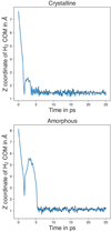 |
Fig. 6 Variation of the z component of the H2 center of mass as a function of time for two sticking trajectories. Points in black represent the position of the maxima. |
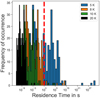 |
Fig. 7 Residence times of H2 on amorphous CO ice. The dashed red line represents a threshold for residence times longer than 1.0 × 10³ s. |
4 Astrophysical implications
The picture created by our simulations points to the conclusion that even with a significant fraction of sticking being present under cold gas and surface conditions (our calculated sticking coefficient for the typical TS = Tg = 10 K conditions is 0.87 for the amorphous ice), residence times on the surface are likely too short to be measured, even considering crystalline CO as the main ice phase under interstellar conditions (Kouchi et al. 2021). Low binding energies are usually correlated with low diffusion barriers, and in the presence of unoccupied deeper binding sites, H2 can therefore diffuse and accommodate for longer times on the surface. In any case, even considering deeper binding sites as the main accommodation sites, our results indicate an extremely weak interaction between H2 and CO. Asmentioned in the introduction, CO is likely the most abundant component of the apolar ice phase (Boogert et al. 2015). Moreover, laboratory studies show little variation in the properties of other apolar ices compared with CO, for example, binding energies or desorption rate constants for the combination of CO/O2/N2 pairs (Öberg et al. 2005; Bisschop et al. 2006; Fuchs et al. 2006). Even though a similar behavior for H2 /O2 and H2 /N2 cannot be taken for granted, it is a fair assumption that binding will in any case be lower than in ASW (− 300 to − 400 K, see Molpeceres & Kästner 2020). One implication of this finding is that H2 adsorption on grains may not be considered homogeneous in translucent and dense clouds, depending on the object’s temperature conditions and dust evolutionary stage, especially in the presence of dust grains with an outer layer consisting of apolar material.
The situation is more complex, however. The processing of CO ice creates impurities with a different binding energy, which affects the distribution of binding sites. UV irradiation, coming from the secondary UV field that permeates dense clouds (Prasad & Tarafdar 1983), has been proven to produce acetaldehyde from mixtures of CH4+CO (Martín-Doménech et al. 2020). Atomic hydrogen is also a crucial processing agent of CO, producing the well-known CO+H →... →CH2O →... →CH3OH sequence through quantum tunneling (Watanabe & Kouchi 2002; Fuchs et al. 2009; Simons et al. 2020). Cosmic rays are also an important agent in CO conversions, with similar implications as photons (Boogert et al. 2015). A recent study of UV irradiation of H2 /CO codeposited mixtures showed rich chemistry for this system owing to the interaction of an electronically excited CO molecule and the H2 molecule (Chuang et al. 2018). Moreover, very recent results are inverting the trend of considering several onion-like models of cold ices (Marchione et al. 2019; Potapov et al. 2020). This new set of experiments shows that small icy domains (clusters or islands) are deposited on top of the refractory phase with voids in between. It should then be possible for the H2 to diffuse in the time frame after a collision and before desorption to deeper binding sites in the complex structure. Furthermore, in H2O/CO ices, CO is not able to cover the full ASW surface, and thus H2 would diffuse to the ASW ice (Kouchi et al. 2021). Incorporating these new paradigms on dust structure into models will require many input parameters, and we consider that our H2 /CO sticking coefficients, binding energies, and residence times will contribute to this goal. There remains an explicit knowledge of diffusivities, which can be estimated according to empirical rules as a fraction of the binding energy (Sandford & Allamandola 1988; Ruffle & Herbst 2000; Cuppen et al. 2009; Chang & Herbst 2012) or be determined by advanced sampling techniques.
It is important to mention that in this study residence times were obtained for almost ideal crystalline ices and compact amorphous ices, and for surface deposition. The structural model presented here ignores possible defects (dislocations or vacancies) in the crystalline structure, the presence of porous domains in the case of the amorphous ices, or the embedding of pre-adsorbed H2 molecules by CO ices (as simulated by codeposition experiments) (Chuang et al. 2018). These defects increase the H2 residence times, as was recently found by experiments showing hydrogenation of CO at temperatures as high as 70 K when CO is embedded in ASW (Tsuge et al. 2020), suggesting deeper potential sites at the mesoscopic scale. Binding energies for H/CO are higher than in the case of H2, with values in the range of −320 K for a flat CO surface or of −440 K, when embedded in a CO layer (Fuchs et al. 2009). When these two findings are combined, the migration of H2 on mixed ices can therefore be safely assumed.
5 Concluding remarks
We extract a series of points from our study that we would like to highlight. We list them below.
- 1.
Our machine-learned potential can reproduce the CO – CO and CO – H2 interaction potential. The results we presented possess DFT quality at a significant fraction of its cost;
- 2.
We have found several possible binding sites of H2 on crystalline CO. Our estimated binding energy is the median of the binding energy distribution, with a value of −266 K. Binding energies on amorphous CO are lower, with an average value of − 157 K, but a broader distribution of binding energies;
- 3.
Theoretical sticking coefficients for the H2/CO system were derived. They are never equal to unity or zero. The effects of gas temperature, surface temperature, and surface phase were considered. All of them are relevant for the value of the sticking coefficients, especially at low gas temperatures;
- 4.
Our residence times, obtained from using our average binding energies in an Arrhenius-like equation, show that in amorphous CO, H2 will desorb in seconds, even at temperatures as low as 5 K. Using the complete average binding energy distribution, we deduce that at low temperatures (≤10 K), the possibility of diffusion to deeper binding sites must be taken into account. In the case of crystalline CO, the distribution is not that broad, and employing the median of the binding energy distribution is justified. Doing so, we obtain residence times on the order of 1 × 10⁻² s at 10 K;
- 5.
In the light of our results, significant adsorption of H2 on top of pure (amorphous or crystalline) CO surfaces is not expected. We hypothesize that in real ices, the distribution of binding sites is greatly affected by the morphology of the ice and the presence of defects and impurities. Therefore our theoretically derived values are of use in the modeling of surface processes on top of realistic interstellar ices.
Further work will include the effect of impurities resulting from ice processing on the distribution of binding energies and sticking coefficients. In addition, the study of explicit diffusion of H2 molecules would be valuable. With knowledge of diffusivities, it would be possible to estimate the fraction of molecules that remain bound in deep minima before the specific time of desorption.
Acknowledgements
We thank the Deutsche Forschungsgemeinschaft (DFG, German Research Foundation) for supporting this work by funding EXC 2075 – 390740016 under Germany’s Excellence Strategy. We acknowledge the support of the Stuttgart Center for Simulation Science (SimTech). We also like to acknowledge the support by the state of Baden-Württemberg through the bwHPC consortium for providing computer and GPU time. G.M. acknowledges the support of the Alexander von Humboldt Foundation through a postdoctoral research grant. V.Z. acknowledges financial support received in the form of a Ph.D. scholarship from the Studienstiftung des Deutschen Volkes (German National Academic Foundation).
Appendix A Choice of DFT functional and accuracy of the MLP
To obtain reliable binding energies and sticking coefficients, we must ensure, on the one hand, the quality of the density functional theory (DFT) method and on the other hand, the quality of the fitted machine-learned potential (MLP). The DFT method of choice (BHLYP-D4) was validated by comparison with more accurate CCSD(T)-F12/cc-pVTZ-F12 calculations (Adler et al. 2007; Peterson et al. 2008; Knizia et al. 2009) on model CO–CO and CO-H2 dimers. In the absence of multireference effects, CCSD(T)-F12 can be considered to have chemical accuracy. CCSD(T)-F12 calculations were made in Molpro2015 (Werner et al. 2012, 2015). The different configurations of the dimers were generated similarly to our previous works (Molpeceres & Kästner 2020; Molpeceres et al. 2020). Briefly, with the center of mass of a CO molecule located at the origin, we place the center of mass of the second molecule (either another CO or H2) at random points of a spherical Fibonacci lattice of a given radius (r). We sampled different r both for CO–CO (r = {2.0, 3.0, 4.0, 5.0, 6.0} Å) and CO–H2 (r = {2.0, 2.5, 3.0, 3.5, 4.0, 4.5, 5.0, 5.5, 6.0}). Twenty-five configurations per radius were considered. The DFT methods under consideration were (1) B3LYP-D4, (2) BHLYP-D4, (3) PBE-D4, (4) BLYP-D4, (5) BP86-D4, (6) PBEh-3c, and (7) B97-3c. Methods (1) to (5) were accompanied by a def2-TZVP basis set, and methods (6) and (7) have predefined basis-sets, def2-mSVP and def2-mTZVP, respectively. The reason for sampling a larger range of configurations for the CO–H2 pair is that all the quantities derived in this work depend on the quality of this particular interaction. The comparison of the different functionals was made on the basis of the mean absolute error (MAE) between the DFT energies and the respective CCSD(T)-F12 energies. The results are presented in Table A.1 for the CO–CO interactions and in Table A.2 for those of CO–H2. From both tables, the choice ofeither one of the hybrid functionals B3LYP-D4 or BHLYP-D4 appears evident. We selected the BHLYP-D4 method because it better describes the CO–H2 interactions at middle ranges. Large deviations at a radius of 2.0 Å arise from configurations in highly repulsive regions.
Benchmark of DFT functionals for the CO-CO interaction.
With the choice of the theoretical method, the next step was to create the training set for the MLP, as described in the main text. The selection of the cutoff radius for the MLP was made based on the average interaction energy of the CO–H2 dimer at long distances. From our CCSD(T)-F12 values of the benchmark, we determined that at a radius of the sphere of 6 Å, the average interaction energy between the two molecules is − 5.3 K, which is approximately half the value of our lowest employed kinetic energy in the collision dynamics. It is worth mentioning that our MLP smoothly decays to zero in the region close to the cutoff radius (Zaverkin & Kästner 2020). This means that even when the dynamics of H2 are incorrect at distances larger than the cutoff radius, the combination of an almost negligible interaction potential and the smoothness of the MLP ensures that the collision dynamics is reasonable. We cannot exclude that larger cutoffs would lead to earlier curvatures in the collision trajectories because of the small (< −5 K) interaction between adsorbate and surface. This change may define a slightly different final collision point with the surface, but we sampled hundreds of collision points per initial kinetic energy, and they were chosen randomly on the surface, so that the sticking results mustremain unaffected.
Benchmark of DFT functionals for the CO–H2 interaction.
Finally, we compared the MLP and the underlying method (BHLYP-D4). As can be observed in Sect. 1, for the training set we used clusters containing at least 10 CO molecules to describe the CO–CO and the CO–H2 interactions.Therefore the potential is not tailored for the comparison between dimers that we presented above. In order to verify the quality of the MLP potential, we confirmed the potential energy profile for a H2 molecule approaching a cluster of 10 CO molecules, which is the cluster size from which data for the CO-H2 interaction are taken from, in addition to checking the overall deviation between independent models to be < ~1 kcal mol−1 Å−1 in the relevant regions of the surface. The procedure is as follows: From a random optimized cluster at the BHLYP-D4 level of theory we ran a (rigid) potential energy scan of a H2 molecule approaching the cluster, both with the MLP and with BHLYP-D4. The results for the comparison are shown in Fig. A.1. From the graph, we observe that the MLP reproduces the physical behavior of the CO–H2 potential up to a resolution of tens of K. The small deviations in the potential arise from the incompleteness of the training set. We sampled other PES scans, which in some cases led to stronger binding than BHLYP-D4 (as shown in Fig. A.1) and in some cases to weaker binding. The deviations that we found are in all cases on the same order (~ 10–20 K), smaller than our uncertainty in the binding energies (75 K, see Fig. 2, bottom panel), so that the possible deviations are averaged out. Therefore we consider our potential suitable for producing simulations.
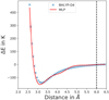 |
Fig. A.1 Potential energy profile for a H2 molecule detaching from a 10 CO cluster. Results are presented with DFT and with our MLP potential. The difference between DFT and MLP minima is 14 K, and in the region between 4–0–5.5 Å, the difference is about 10 K. The dotted black line represents the training cutoff. |
References
- Abadi, M., Agarwal, A., Barham, P., et al. 2015, TensorFlow: Large-Scale Machine Learning on Heterogeneous Systems, software available from https://www.tensorflow.org/about/bib [Google Scholar]
- Acharyya, K. 2014, MNRAS, 443, 1301 [Google Scholar]
- Adler, T. B., Knizia, G., & Werner, H.-J. 2007, J. Chem. Phys., 127, 221106 [Google Scholar]
- Álvarez-Barcia, S., Russ, P., Kästner, J., & Lamberts, T. 2018, MNRAS, 479, 2007 [Google Scholar]
- Balasubramani, S. G., Chen, G. P., Coriani, S., et al. 2020, J. Chem. Phys., 152, 184107 [Google Scholar]
- Becke, A. D. 1993, J. Chem. Phys., 98, 1372 [NASA ADS] [CrossRef] [Google Scholar]
- Bisschop, S. E., Fraser, H. J., Öberg, K. I., Van Dishoeck, E. F., & Schlemmer, S. 2006, A&A, 449, 1297 [NASA ADS] [CrossRef] [EDP Sciences] [Google Scholar]
- Boogert, A. C., Gerakines, P. A., & Whittet, D. C. 2015, ARA&A, 53, 541 [Google Scholar]
- Bron, E., Le Petit, F., & Le Bourlot, J. 2016, A&A, 588, A27 [NASA ADS] [CrossRef] [EDP Sciences] [Google Scholar]
- Buch, V., & Zhang, Q. 1991, ApJ, 379, 647 [Google Scholar]
- Caldeweyher, E., Ehlert, S., Hansen, A., et al. 2019, J. Chem. Phys., 150, 154122 [Google Scholar]
- Chang, Q., & Herbst, E. 2012, ApJ, 759, 147 [Google Scholar]
- Chuang, K.-J., Fedoseev, G., Qasim, D., et al. 2018, A&A, 617, A87 [NASA ADS] [CrossRef] [EDP Sciences] [Google Scholar]
- Cuppen, H. M., Van Dishoeck, E. F., Herbst, E., & Tielens, A. G. 2009, A&A, 508, 275 [NASA ADS] [CrossRef] [EDP Sciences] [Google Scholar]
- Fuchs, G. W., Acharyya, K., Bisschop, S. E., et al. 2006, Faraday Discuss., 133, 331 [Google Scholar]
- Fuchs, G. W., Cuppen, H. M., Ioppolo, S., et al. 2009, A&A, 505, 629 [NASA ADS] [CrossRef] [EDP Sciences] [Google Scholar]
- Fukutani, K., & Sugimoto, T. 2013, Prog. Surface. Sci., 88, 279 [Google Scholar]
- Govers, T. R., Mattera, L., & Scoles, G. 1980, J. Chem. Phys., 72, 5446 [NASA ADS] [CrossRef] [Google Scholar]
- Hanwell, M. D., Curtis, D. E., Lonie, D. C., et al. 2012, J. Cheminformatics, 4, 17 [Google Scholar]
- He, J., Acharyya, K., & Vidali, G. 2016a, ApJ, 823, 56 [Google Scholar]
- He, J., Acharyya, K., & Vidali, G. 2016b, ApJ, 825, 89 [Google Scholar]
- Hjorth Larsen, A., JØrgen Mortensen, J., Blomqvist, J., et al. 2017, J. Condens. Matter Phys., 29, 273002 [Google Scholar]
- Karssemeijer, L. J., Ioppolo, S., van Hemert, M. C., et al. 2014, ApJ, 781, 16 [Google Scholar]
- Knizia, G., Adler, T. B., & Werner, H.-J. 2009, J. Chem. Phys., 130, 054104 [Google Scholar]
- Kouchi, A. 1990, J. Cryst. Growth, 99, 1220 [Google Scholar]
- Kouchi, A., Tsuge, M., Tetsuya, H., et al. 2021, MNRAS, submitted [Google Scholar]
- Krupskii, I. N., Prokhvatilov, A. I., Erenburg, A. I., & Yantsevich, L. D. 1973, Phys. Status Solidi A, 19, 519 [Google Scholar]
- Lamberts, T., & Kästner, J. 2017, J. Phys. Chem. A, 121, 9736 [Google Scholar]
- Lamberts, T., Markmeyer, M. N., Kolb, F. J., & Kästner, J. 2019, ACS. Earth. Space. Chem., 3, 958 [Google Scholar]
- Lauck, T., Karssemeijer, L., Shulenberger, K., et al. 2015, ApJ, 801, 118 [Google Scholar]
- Marchione, D., Rosu-Finsen, A., Taj, S., et al. 2019, ACS. Earth. Space. Chem., 3, 1915 [Google Scholar]
- Maret, S., & Bergin, E. A. 2007, ApJ, 664, 956 [Google Scholar]
- Martín-Doménech, R., Öberg, K. I., & Rajappan, M. 2020, ApJ, 894, 98 [Google Scholar]
- Martinez, L., Andrade, R., Birgin, E. G., & Martínez, J. M. 2009, J. Comp. Chem., 30, 2157 [Google Scholar]
- Matar, E., Bergeron, H., Dulieu, F., et al. 2010, J. Chem. Phys., 133, 104507 [Google Scholar]
- Meisner, J., Lamberts, T., & Kästner, J. 2017, ACS Earth Space. Chem, 1, 399 [Google Scholar]
- Metz, S., Kästner, J., Sokol, A. A., Keal, T. W., & Sherwood, P. 2014, Wiley Interdiscip. Rev. Comput. Mol. Sci., 4, 101 [Google Scholar]
- Molpeceres, G., & Kästner, J. 2020, Phys. Chem. Chem. Phys., 22, 7552 [Google Scholar]
- Molpeceres, G., Zaverkin, V., & Kästner, J. 2020, MNRAS, 499, 1373 [Google Scholar]
- Oba, Y., Tomaru, T., Lamberts, T., Kouchi, A., & Watanabe, N. 2018, Nat. Astron., 2, 228 [NASA ADS] [CrossRef] [Google Scholar]
- Öberg, K. I., van Broekhuizen, F., Fraser, H. J., et al. 2005, ApJ, 621, L33 [NASA ADS] [CrossRef] [Google Scholar]
- Pagani, L., Vastel, C., Hugo, E., et al. 2009, A&A, 494, 623 [NASA ADS] [CrossRef] [EDP Sciences] [Google Scholar]
- Peterson, K. A., Adler, T. B., & Werner, H.-J. 2008, J. Chem. Phys., 128, 084102 [Google Scholar]
- Potapov, A., Jäger, C., & Henning, T. 2020, Phys. Rev. Lett., 124, 221103 [Google Scholar]
- Prasad, S. S., & Tarafdar, S. P. 1983, ApJ, 267, 603 [Google Scholar]
- Reddi, S. J., Kale, S., & Kumar, S. 2019, ArXiv e-prints [arXiv:1904.09237] [Google Scholar]
- Ruffle, D. P., & Herbst, E. 2000, MNRAS, 319, 837 [Google Scholar]
- Sandford, S. A., & Allamandola, L. J. 1988, Icarus, 76, 201 [NASA ADS] [CrossRef] [Google Scholar]
- Seabold, S., & Perktold, J. 2010, in 9th Python in Science Conference [Google Scholar]
- Sherwood, P., De Vries, A. H., Guest, M. F., et al. 2003, J. Mol. Struct., 632, 1 [Google Scholar]
- Shimonishi, T., Nakatani, N., Furuya, K., & Hama, T. 2018, ApJ, 855, 27 [Google Scholar]
- Simons, M. A., Lamberts, T., & Cuppen, H. M. 2020, A&A, 634, A52 [CrossRef] [EDP Sciences] [Google Scholar]
- Spicher, S., & Grimme, S. 2020, Angew. Chem. Int. Ed., 59, 15665 [Google Scholar]
- Troscompt, N., Faure, A., Maret, S., et al. 2009, A&A, 506, 1243 [NASA ADS] [CrossRef] [EDP Sciences] [Google Scholar]
- Tsuge, M., Hidaka, H., Kouchi, A., & Watanabe, N. 2020, ApJ, 900, 187 [Google Scholar]
- Ueta, H., Watanabe, N., Hama, T., & Kouchi, A. 2016, Phys. Rev. Lett., 116, 25 [Google Scholar]
- Van Hemert, M. C., Takahashi, J., & Van Dishoeck, E. F. 2015, J. Phys. Chem. A., 119, 6354 [Google Scholar]
- Vegard, I. 1930, Z. Phys., 61, 185 [Google Scholar]
- Wakelam, V., Herbst, E., Loison, J.-C., et al. 2012, ApJS, 199, 21 [NASA ADS] [CrossRef] [Google Scholar]
- Wakelam, V., Bron, E., Cazaux, S., et al. 2017, Mol. Astrophys., 9, 1 [Google Scholar]
- Watanabe, N., & Kouchi, A. 2002, ApJ, 571, L173 [Google Scholar]
- Watanabe, N., Kimura, Y., Kouchi, A., et al. 2010, ApJ, 714, L233 [Google Scholar]
- Weigend, F., & Ahlrichs, R. 2005, Phys. Chem. Chem. Phys., 7, 3297 [Google Scholar]
- Werner, H.-J., Knowles, P. J., Knizia, G., Manby, F. R., & Schütz, M. 2012, WIREs Comput. Mol. Sci., 2, 242 [CrossRef] [Google Scholar]
- Werner, H.-J., Knowles, P. J., Knizia, G., et al. 2015, MOLPRO, version 2015.1, a package of ab initio programs [Google Scholar]
- Zaverkin, V., & Kästner, J. 2020, J. Chem. Theory Comput., 16, 5410 [Google Scholar]
All Tables
Structures, temperatures (T, in K), and time interval between snapshots extraction for refinement (f, in fs) and total number of structures (N) included in the training set to construct the neural network potential.
Summary of the sticking probabilities (P(E)) obtained in this work as a function of the ice phase, particle incoming energy (E), and surface temperature (TS).
Summary of the sticking coefficients (ST) obtained in this work as a function of the ice phase, gas temperature (Tg), and surface temperature (TS).
All Figures
|
Fig. 1 Side and top views of the relaxed carbon monoxide ice surface models employed in our simulations. On the left we show the crystalline surface, and on the right the amorphous surface. |
| In the text | |
|
Fig. 2 Distribution of binding energies for the H2/CO system. In the upper panel for a crystalline surface, and in the lower panel for an amorphous one. |
| In the text | |
|
Fig. 3 Adsorption sites for the H2 molecule on top of crystalline CO. Left panel: top, middle panel: bridge. Right panel: hollow. |
| In the text | |
|
Fig. 4 Sticking probabilities P(E) of the H2/CO system at different surface temperatures. Left panel: crystalline sample. Right panel: amorphous sample. |
| In the text | |
|
Fig. 5 Integrated sticking coefficients ST of the H2/CO system at different surface temperatures. Left panel: crystalline sample. Right panel: amorphous sample. All curves start at Tg = TS. |
| In the text | |
|
Fig. 6 Variation of the z component of the H2 center of mass as a function of time for two sticking trajectories. Points in black represent the position of the maxima. |
| In the text | |
|
Fig. 7 Residence times of H2 on amorphous CO ice. The dashed red line represents a threshold for residence times longer than 1.0 × 10³ s. |
| In the text | |
|
Fig. A.1 Potential energy profile for a H2 molecule detaching from a 10 CO cluster. Results are presented with DFT and with our MLP potential. The difference between DFT and MLP minima is 14 K, and in the region between 4–0–5.5 Å, the difference is about 10 K. The dotted black line represents the training cutoff. |
| In the text | |
Current usage metrics show cumulative count of Article Views (full-text article views including HTML views, PDF and ePub downloads, according to the available data) and Abstracts Views on Vision4Press platform.
Data correspond to usage on the plateform after 2015. The current usage metrics is available 48-96 hours after online publication and is updated daily on week days.
Initial download of the metrics may take a while.