| Issue |
A&A
Volume 647, March 2021
|
|
|---|---|---|
| Article Number | A149 | |
| Number of page(s) | 12 | |
| Section | The Sun and the Heliosphere | |
| DOI | https://doi.org/10.1051/0004-6361/202039867 | |
| Published online | 26 March 2021 | |
Over-expansion of a coronal mass ejection generates sub-Alfvénic plasma conditions in the solar wind at Earth
1
Centre for mathematical Plasma Astrophysics, Dept. of Mathematics, KU Leuven, Celestijnenlaan 200B, 3001 Leuven, Belgium
e-mail: Emmanuel.Chane@kuleuven.be
2
LESIA, Observatoire de Paris, PSL Research University, CNRS Sorbonne Université, Univ. Paris 06, Univ. Paris Diderot, Sorbonne Paris Cité, 5 place Jules Janssen, 92195 Meudon, France
3
CONICET, Universidad de Buenos Aires, Instituto de Astronomía y Física del Espacio, LAMP Group, CC. 67, Suc. 28, 1428 Buenos Aires, Argentina
4
Universidad de Buenos Aires, Facultad de Ciencias Exactas y Naturales, Departamento de Ciencias de la Atmósfera y los Océanos and Departmento de Física, LAMP Group, 1428 Buenos Aires, Argentina
5
Department of Space Physics, Institute of Atmospheric Physics of the Czech Academy of Sciences, Prague, Czech Republic
6
Laboratoire Cogitamus, 1 3/4 rue Descartes, 75005 Paris, France
7
Institute of Physics, University of Maria Curie-Skłodowska, ul. Radziszewskiego 10, 20-031 Lublin, Poland
Received:
6
November
2020
Accepted:
18
January
2021
Context. From May 24–25, 2002, four spacecraft located in the solar wind at about 1 astronomical unit (au) measured plasma densities one to two orders of magnitude lower than usual. The density was so low that the flow became sub-Alfvénic for four hours, and the Alfvén Mach number was as low as 0.4. Consequently, the Earth lost its bow shock, and two long Alfvén wings were generated.
Aims. This is one of the lowest density events ever recorded in the solar wind at 1 au, and the least documented one. Our goal is to understand what caused the very low density.
Methods. Large Angle and Spectrometric Coronagraph (LASCO) and in situ data were used to identify whether something unusual occurred that could have generated such low densities
Results. The very low density was recorded inside a large interplanetary coronal mass ejection (ICME), which displayed a long, linearly declining velocity profile, typical of expanding ICMEs. We deduce a normalised radial expansion rate of 1.6. Such a strong expansion, occurring over a long period of time, implies a radial size expansion growing with the distance from the Sun to the power 1.6. This can explain a two-orders-of-magnitude drop in plasma density. Data from LASCO and the Advanced Composition Explorer show that this over-expanding ICME was travelling in the wake of a previous ICME.
Conclusions. The very low densities measured in the solar wind in May 2002 were caused by the over-expansion of a large ICME. This over-expansion was made possible because the ICME was travelling in a low-density and high-velocity environment present in the wake of another ICME coming from a nearby region on the Sun and ejected only three hours previously. Such conditions are very unusual, which explains why such very low densities are almost never observed.
Key words: Sun: coronal mass ejections (CMEs) / Sun: infrared / solar wind / magnetohydrodynamics (MHD)
© ESO 2021
1. Introduction
Starting on 2002 May 24 at approximately 22:00 UTC, the solar wind conditions around the Earth were extremely unusual: its density was two orders of magnitude lower than average, and, as a result, the solar wind became sub-Alfvénic for four hours, with values as low as 0.4 for the Alfvén Mach number (see Chané et al. 2012). This very low density was measured consistently by four independent spacecraft, namely the Advanced Composition Explorer (ACE), GENESIS, the Solar and Heliospheric Observatory (SOHO), and WIND. Low-density events in the solar wind upstream of the Earth’s magnetosphere were studied by Usmanov et al. (2005). They analysed data between 1963 and 2003 and found 23 events where the density in the solar wind was lower than 0.3 cm−3. Sub-Alfvénic conditions were present in nine of these events. More recently, Chané et al. (2017) analysed 52 years of solar wind measurements and found that long lasting (> 1 h) low density solar wind events at Earth that result in sub-Alfvénic conditions only occur, on average, every 2.2 years.
The most famous example of such low density sub-Alfvénic events was entitled ‘the day the solar wind almost disappeared’, which occurred on 1999 May 11. But this event, which has been studied by Farrugia et al. (2000), Lazarus (2000), Le et al. (2000a,b), and Smith et al. (2001) is by no means the most extreme of the low-density events in the solar wind. During the year 1979, for instance, three very-low-density events were measured at 1 astronomical unit (au): on July 4, July 31, and November 22 (Crooker et al. 2000; Gosling et al. 1982). The November event is interesting because the low-density, sub-Alfvénic flow was already measured by the Helios 2 spacecraft at 0.3 au on November 13 (Schwenn 1983). Unusually low densities in the solar wind have also been measured at higher latitudes. Riley et al. (1998) analysed Ulysses data, when the spacecraft was at 3.7 au and at N38.5° latitude on 1996 May 01. They found a time period of 3.5 hours when the solar wind density was ten times lower than typical and called it a ‘density hole’. As mentioned before, another example of a very-low-density, sub-Alfvénic event at 1 au happened in May 2002, when the solar wind was peculiar for a long period of time: the density was lower than 0.5 cm−3 (ten times lower than usual) for more than 40 hours, which resulted in an Alfvén Mach number lower than 2.
The configuration of Earth’s magnetosphere changes drastically when it is embedded in a low density, sub-Alfvénic solar wind. For example, the distance between the bow shock and the magnetopause is strongly influenced by the upstream Alfvén Mach number. Under usual circumstances, this distance is about 4 RE (Fairfield 1971), where RE denotes the radius of the Earth, but it increases when the Alfvén Mach number decreases. When the Mach number becomes lower than one, theoretically, the bow-shock moves away to infinity (Farris & Russell 1994). This means that there is no bow-shock and no magnetosheath. The solar wind can then reach Earth’s magnetopause directly. For the May 2002 event, Chané et al. (2012) used ACE data at L1 and Geotail data closer to the Earth’s magnetopause to show that there was indeed no strong shock between the two spacecraft, since there was no increase in the magnetic field magnitude. Because the solar wind dynamic pressure is lower than usual during such events, the magnetopause stand-off distance also increases. Chané et al. (2012) calculated that the magnetopause stand-off distance reached 22 RE during the May 2002 event (while it is 11 RE under normal solar wind conditions, see Fairfield 1971).
Another consequence of such sub-Alfvénic solar wind conditions is that two Alfvén wings are generated. These tubular structures, where the incoming plasma is decelerated and where the interplanetary magnetic field experiences a rotation, can be hundreds of vE long (see Drell et al. 1965; Neubauer 1980, 1998, for a theoretical description of the Alfvén wings). In the Solar System, Alfvén wings are present for a lot of moons of the giant planets (e.g., Io, Europa, Enceladus). This is because these moons are located inside the magnetosphere of their parent planet where the plasma flow is sub-Alfvénic. These Alfvén wings are well understood and have been thoroughly studied via in situ measurements (Kivelson et al. 1998; Saur et al. 2002), remote sensing observations (Clarke et al. 1996; Gérard et al. 2002), analytical modelling (Neubauer 1998; Saur et al. 1998), and numerical simulations (Linker et al. 1988; Blöcker et al. 2016). At Earth, since they are so rare, we only have one single study providing direct observational evidence of these Alfvén wings (Chané et al. 2012). The evidence came from the spacecraft Geotail, which clearly crossed one of the wings nine times in May 2002. Whereas Alfvén wings are very rare at Earth and at the other planets in our Solar System, they are present on 35% of the exoplanets discovered before 2012 November 14 (Saur et al. 2013, 2018).
While the consequences of the low density event in May 2002 have been thoroughly studied (Chané et al. 2012, 2015), its origin remains unclear. While Chané et al. (2012) briefly mentioned that such a low-density event ‘may have been caused by a complex interaction of CMEs prior to the event’ and that it ‘may have its origin in a long-lasting structure located on the Sun’, they do not provide a physical explanation of how such a low plasma density could have been generated. Janardhan et al. (2008) studied three low-density events (including the May 2002 event) and proposed that they may be related to a transient coronal hole visible at the solar disk centre. In the present paper, we demonstrate that the over-expansion of an ICME during its propagation between the Sun and the Earth is responsible for the low density measured on 2002 May 24–25. We show that the ICME was large (radial size > 0.5 au) when it reached the Earth and that the low-density region was located inside the strongly expanding magnetic ejecta. We calculated the expansion rate of the ICME and established that the solar wind conditions upstream of this ICME were favourable for such an over-expansion. To this end, we demonstrate that the over-expanding ICME was propagating in the low-density and high-velocity environment of a previous ICME’s wake.
Over-expansions in ICMEs were first observed by Gosling et al. (1994, 1998). Over-expansion is characterised by a large difference of velocity between the ICME front and the rear, and by a forward-reverse shock pair delimiting the ICME. Using measurements from the Ulysses spacecraft, they showed that over-expansion was rather common in high-latitude ICMEs. More recently, Démoulin & Dasso (2009) developed an analytical model for the evolution of flux ropes embedded in the solar wind. In this model, cylindrical flux ropes are modelled as a series of force-free field states, with a pressure balance between the ambient solar wind and the flux rope boundary. They showed that, in most cases, the main driver for the expansion of the flux rope is the rapid radial variation of the solar wind total pressure with solar distance, and that an internal overpressure is usually not necessary to model the observed expansion of the flux rope. In all the cases considered in this model, the resulting velocity profile of the flux ropes is found to be very similar and produces a nearly linear decrease of the velocity in time-series. The expansion rate predicted by this model is in good agreement with the observations (see, i.e. Démoulin et al. 2008; Gulisano et al. 2010). The expansion rate of a flux rope affects how its internal magnetic field, density, and pressure evolve during its propagation, and the model of Démoulin & Dasso (2009) can be used to quantify this evolution.
The present paper is organised as follows: the solar observations (flares, coronal hole, CMEs) on 2002 May 21-22 are presented in Sect. 2. In Sect. 3, the in situ measurements at L1 are analysed. The interpretation of the low-density solar wind due to the expansion of the interplanetary flux rope resulting from a complex of CMEs is discussed in Sect. 4. Finally, our conclusions are presented in Sect. 5.
2. Coronal mass ejection and solar source observations
In order to understand the propagation of the CMEs initiated at the Sun’s surface and their expansion in the heliosphere related to the low density solar wind event, we first analysed the solar activity during this period of time, which is reported in the CDAW data center at NASA Goddard in the list of CMEs, and in the list of X-ray flares recorded by the Geostationary Operational Environmental Satellite (GOES) satellite1. In 2002, solar remote-sensing observations were still relatively limited. We used data from the Extreme Ultraviolet Imaging Telescope (EIT; Delaboudinière et al. 1995), providing continuous 2D images of the Sun in EUV wavelengths (195 Å), and the Large Angle and Spectrometric Coronagraph (LASCO; Brueckner et al. 1995), providing images of the solar corona, both of which are onboard SOHO (Fleck et al. 1995). LASCO and EIT (filter at 195 Å) observed images with a common cadence of 12 minutes, and movies of this event are available online2. LASCO consists of two coronagraphs, C2 and C3, with C2 observing the corona until 3 R⊙, and C3 from 3 to 32 R⊙, where R⊙ denotes the radius of the Sun. According to the statistics of CME speeds and based on the ballistic velocity method, we searched the solar events in a window from two to three days (Schmieder et al. 2020). Therefore, we started our search for CMEs that could be related to the weak solar wind event, from 2002 May 21 onwards. The Hα and Ca II K images are found in the Meudon survey database3. The MDI magnetograms come from the solar monitor database4.
Between May 21 at 21:50 UTC and May 22 at 04:00 UTC, LASCO observed three CMEs (Fig. 1 and Table 1). The first CME, called CME0, seen in the north-east limb at 21:50 UTC is associated with a, M1.5 X-ray class flare occurring in the active region (AR) NOAA 9960 located in the solar disk at N17E38 in heliographic coordinates according the CDAW data center (Fig. 1, bottom panel). The source of this CME is located in a different region than the ones of the other two CMEs, which are close to the west limb.
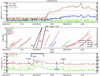 |
Fig. 1. Events of 2002 May 21–22. Top panel: solar energetic particles (SEP) for three frequency bands. Middle panel: trajectories of the studied CMEs, respectively, CME0, CME1, and CME2. Bottom panel: X-ray flares. The class of the three involved flares is indicated at the peaks in the green curve. |
Solar sources, flares related to the CMEs, and their characteristics from 2002 May 21–22.
The first west CME, CME1, is seen on May 21 from 23:50 UTC and is associated with a C9.7 X-ray class flare, due to their simultaneity (Cheng et al. 2005). The CME and flare times are indicated by CME1 and C9.7 in Fig. 1 in the middle and bottom panels, respectively. The origin of the flare and of CME1 is located in the AR NOAA 9948 near the west solar limb at S25W64 (Figs. 2a,b). In the EIT image, weak loops are observed over the limb around the location S25 in heliographic coordinates and these correspond to post flare loops of the flare. This correspondence is confirmed by looking at the 195 Å EIT movie.
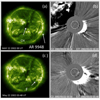 |
Fig. 2. Solar disk observations. (a) and (c): EIT solar disk in the 195Å filter. (b) and (d): LASCO coronagraph C2 showing the two west CMEs when they are well developed in the field of view. White arrows in panel a indicate the AR 9948 near the west limb, and a transient coronal hole (CH) in the centre of the disk. In panel c, the white arrow indicates the region with two parallel bright ribbons after the filament eruption. |
The second west CME, CME2, is associated with a class C5 X-ray flare, indicated as CME2 and C5 in Fig. 1 middle and bottom panels, respectively. CME2 is a full halo CME observed on May 22 at 03:50 UTC (Fig. 2d, Fig. 1 of Cheng et al. 2005). By 04:06 UTC, the C2 occulting disk was surrounded by a thick bright front in the west extending over both poles, with fainter extensions in the east (Fig. 1 of Cheng et al. 2005). The front appeared in LASCO C3 at 03:42 UTC with full coverage of the C3 occultor by 04:18 UTC. The plane of sky front is reported in the GOES catalogue at PA 237 (S33).
The full halo CME2 is principally associated with a large, bright, fast prominence eruption that EIT observed between 03:00 and 04:24 UTC (see the EIT movie and Fig. 3). GOES notes a disappearing filament between 03:18 and 05:00 UTC associated with a C5.0 X-ray class flare between 03:18 and 05:02 UTC with a peak emission at 03:54 UTC. The eruption and the flare could be considered effectively as associated phenomena due to their similar time onset in view of the low cadence of the observations. The reconnection should occur just before 03:36 UTC and could correspond to the registered C5 flare by GOES. It corresponds to a long duration flare indicated by C5 in the bottom panel of Fig. 1. In the EIT movie the filament is rising between 03:00 and 03:24 UTC. At 03:36 UTC, double bright parallel ribbons with loops joining both of them can be seen. The loops rise for a long time until 11:00 UTC and appear over the limb. The filament eruption is also observed in radio wavelengths (Nobeyama at 17 GHz) between 03:05 and 03:25 UTC (Fig. 3, panels d and e). The prominence, observed a few days before its eruption as a filament, is extended in a long region of the disk centred at S19W56 and extended over 40 degrees (S19 ± 20 degrees). This long region is oriented north-west, south-east between relatively weak magnetic field regions (< 1000 Gauss) along the east side of the AR 9948 (Figs. 3a–c,f and Fig. 5 of Cheng et al. 2005). This long filament is classified as sinistral from the spatial organisation of its feet/barbs (Pevtsov 2002). This implies a positive helicity for the associated magnetic configuration. In the solar disk observed on 2002 May 22 shown in Fig. 2 (panels a and c), a transient coronal hole faces towards the Earth and could possibly play a role in explaining the low-density solar wind as proposed by Janardhan et al. (2008).
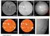 |
Fig. 3. Solar disk observations. (a): longitudinal magnetic field from MDI on May 22 with the active region (AR) numbers. (b) and (c): Meudon spectroheliogram observations in Ca II and Hα, respectively, showing the long filament (F) in the west in Hα. (d) and (e): radio images in 17 GHz obtained in Nobeyama showing the filament eruption between 03:05 and 3:25 UTC. (f): zoom in Hα on the filament and AR 9948. |
Due to the extents of the two partial halo CMEs, CME0 and CME1, and to the positions of their apparent source regions, either one or both might have a small Earth-directed component. The speeds of the two partial halo CMEs average 853 km s−1 and 1246 km s−1 according to the GOES catalogue (Table 1). Both could likely be overtaken by CME2 with its speed around 1557 km s−1, which is much faster than the two earlier CMEs. CME2 is seen running into CME1 in the outer region of the C3 field of view, and CME0 is significantly slower. However, CME0’s propagation direction is observed in C2 is towards the east, and it is only a partial CME, so there is only a slight chance of CME2 overtaking CME0. Therefore, the two events with a source in the west were labelled as sympathetic, homologous events by Cheng et al. (2005). Their detailed analysis of the speed between C2 and C3 leads to the conclusion that the speed increased from 937 km s−1 to 1243 km s−1 for CME1 and from 1400 km s−1 to 1740 km s−1 for CME2. Therefore, a single complex ejecta at 1 au, formed by CME1 overtaken by CME2, is the most likely outcome of these three CMEs.
The CMEs, CME1 and CME2, and most likely their associated flares, have implications in the level of energetic particles detected at 1 au (Fig. 1, top panel). In the GOES curve of low-energy SEPs (in red) there is a first rise of SEP intensity with a plateau at about 5 cm−2 s−1 sr−1, then a second rise with a plateau at approximately 100 cm−2 s−1 sr−1, and finally a maximum near 900 cm−2 s−1 sr−1 on May 23 just before 12:00 UTC (Fig. 1). This last maximum is commonly interpreted as an energetic storm particle event (ESP). The particles are trapped in the ICME shock and are locally accelerated in the vicinity of the Earth (Mäkelä et al. 2011).
3. Observations at L1 and geoeffectivity
3.1. Overview: Two geoeffective ICMEs
Figure 4 displays in situ measurements obtained at L1 by the spacecraft ACE between 2002 May 23 and 2002 May 26. These measurements show the observations of two successive ICMEs (ICME1 and ICME2). On May 23, before 10:15 UTC, the spacecraft was embedded in a slow solar wind (∼420 km s−1), where the plasma number density and the magnetic field strength are slightly above average: about 10 cm−3 and 15 nT, respectively. At 10:15 UTC, an interplanetary shock reaches the spacecraft: the plasma density jumps to 25 cm−3, the field strength to approximately 40 nT, and the plasma speed to 580 km s−1. The ACE spacecraft is then located in the sheath of ICME1 (blue background in Fig. 4), until 2002 May 23 at 11:50 UTC, when it enters the magnetic ejecta of ICME1 (yellow background in Fig. 4). The liberation of the energetic particles on May 23 at 12:00 UTC (see the maximum of the SEP curve in Fig. 1), that is defined as an energetic storm particle event, occurs just at the front of the first ejecta. This agrees well with the timing of the first ejecta that we propose. This ejecta is characterised by a rotating magnetic field (very clear for the Y- and Z-components), an average speed of ∼800 km s−1, and by a lower plasma density: around 2 cm−3. The spacecraft stays within the ejecta for three hours. The expected temperature is also plotted in panel d of Fig. 4 (see Lopez & Freeman 1986; Lopez 1987, for more details). We note that the ratio between the plasma temperature and the expected temperature is relatively high for this magnetic ejecta. Nevertheless, based on the aforementioned rotating magnetic field, we are still convinced that the spacecraft is located inside the magnetic ejecta. Furthermore, in Fig. 4, panel d, the plasma temperature is compared to half of the expected temperature. Here, we followed the notion of Richardson & Cane (1995) that in the interplanetary space a plasma temperature below half the expected one is abnormally cold and is probably not from a quiet solar wind region.
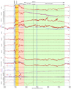 |
Fig. 4. ACE in situ measurements at L1 and geomagnetic indices. (a) The number density (in cm−3) on a logarithmic scale; (b) the plasma speed (in red) and a straight line (indigo) that has been added to illustrate the very long, almost linear plasma-speed decrease between 2002 May 23 at 22:54 UTC and 2002 May 25 at 10:35 UTC; (c) the Alfvén speed; (d) the plasma temperature (in red) and half the expected plasma temperature (in blue) on a logarithmic scale; (e) the magnetic field strength on a logarithmic scale; (f), (g), and (h) the components of the magnetic field in GSE; (i) the plasma β; (j) the thermal (in red), magnetic (in blue), and total (in grey) pressures (in pPa); (k) the disturbance storm time (Dst) index (in red) and SYM-H indices (in blue); (l) the AE (in red), AU (in blue), and AL (in grey) auroral indices; (m) the Pearson product-moment correlation coefficient for the plasma speed and the plasma temperature for a moving time window of six hours. The background colours illustrate the different structures in the solar wind: the sheath of the first ICME is in light blue (on 2002 May 23 between10:15 UTC and 11:50 UTC); the magnetic ejecta of the first ICME is in yellow (on 2002 May 23 between 11:50 UTC and 15:10 UTC); the sheath of the second ICME is in light red (on 2002 May 23 between 15:10 UTC and 21:30 UTC); the magnetic ejecta of the second ICME is in light green (between the 2002 May 23 at 21:30 UTC and the 2002 May 25 at 18:00 UTC). The end of the second flux rope is represented by a vertical black line. The flux rope back itself is separated into two regions by a vertical blue line. |
On 2002 May 23 at about 15:10 UTC, a sharp increase (jump) is seen in the plasma density and velocity, while the temperature suddenly decreases, and the components of the magnetic field change, while |B| only slightly changes (Fig. 4). Although the jump at 15:10 UTC is not a shock, the structure following it (with the red background in Fig. 4) has the characteristics of a sheath. The absence of a shock in front of ICME2 can be explained as follows: even though the ejecta of ICME2 displays a high velocity, it travels in a very depleted plasma with a rather strong magnetic field (yellow region in Fig. 4). This means that the Alfvén speed upstream of IMCE 2 is high (400–600 km s−1, see Fig. 4, panel c). In addition, this plasma displays a high velocity, and the speed difference between the ICME and the upstream plasma is only about 200 km s−1 (Fig. 4, panel b). The plasma speed difference is thus lower than the Alfvén speed (and therefore lower than the fast magnetosonic speed), hence no shock is generated in front of ICME2. On the other hand, it is entirely possible that ICME2 had a shock before reaching ACE, since the upstream conditions were different. In that context, this shock may have propagated through ICME1 and may even have merged with the shock in front of ICME1 (see Lugaz et al. 2005; Scolini et al. 2020a, for more details on shock magnetic cloud interactions).
On 2002 May 23 at 21:30 UTC (in agreement with Nieves-Chinchilla et al. 2018, for a 32 min delay between ACE and WIND), ACE enters the ejecta of the second ICME (ICME2). It remains inside it for more than 44 hours until 2002 May 25 at 18:00 UTC (green background in Figs. 4 and 5). This particular ejecta is characterised by a very long and linear velocity decrease (from 850 km s−1 to 350 km s−1, see panel b in Fig. 5), by an unusually low plasma density (always below 0.8 cm−3 and sometimes as low as 0.04 cm−3), and by a very smooth magnetic field (see panels e to h in Fig. 5). In Sect. 4, we show how this velocity difference between the front and the back of the ejecta leads to the very low density measured by the spacecraft. Similar ejecta were observed by Gosling et al. (1994) with the Ulysses spacecraft in June 1993, when Ulysses was located at 4.64 au and at a heliographic latitude of S32.5°. They observed an ejecta with an abnormally low density, a long smooth linearly declining velocity profile, and a low variance magnetic field. Interestingly, this event was associated with a pair of forward-reverse shocks, similar to those usually observed in corotating interaction regions. Next, as can be seen in Figs. 4 and 5, the linear velocity profile (highlighted with the indigo straight line) is only present for 80% of the ejecta, and, in particular, the profile is rather flat in the rear. This might be caused by the interaction with the faster, trailing solar wind. Such so-called perturbed events are frequent in the inner heliosphere (about half of the cases, see Gulisano et al. 2010).
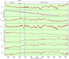 |
Fig. 5. ACE in situ measurements at L1. (a) The number density (in cm−3) on a logarithmic scale; (b) the plasma speed (in red) and a straight line (indigo) that has been added to illustrate the very long, almost linear plasma-speed decrease between 2002 May 23 at 22:54 UTC and 2002 May 25 at 10:35 UTC; (c) the plasma temperature on a logarithmic scale; (d) the plasma beta on a logarithmic scale; (e) the magnetic field strength; (f), (g), and (h) the components of the magnetic field in GSE. The background colours illustrate the different structures in the solar wind: the sheath of the second ICME is in light red (on 2002 May 23 between 15:10 UTC and 21:30 UTC); the magnetic ejecta of the second ICME is in light green (between the 2002 May 23 at 21:30 UTC and the 2002 May 25 at 18:00 UTC). The end of the second flux rope is represented by a vertical black line. The flux rope back itself is separated into two regions by a vertical blue line. |
For the May 2002 event, one can see in Fig. 5 that a flux rope is present in the front of the ejecta, where a fully coherent magnetic field can be seen between 2002 May 23 at 21:30 UTC and 2002 May 24 at about 8:00 UTC. During this time interval, the magnetic field turns from southward (Bz ≃ −2 nT) to northward (Bz ≃ 2 nT), whereas Bx remains negative (Bx ∈ [ − 11; −10] nT) and By stays positive (By ∈ [0; 4] nT), as seen in Fig. 5. This is coherent with ACE going through the northern part of the flux rope. Since one of the azimuthal components (Bx) clearly dominates the axial component of the flux rope (By), the spacecraft did not pass close to the centre of the flux rope, and we thus have a large impact parameter. Indeed, with a Lundquist flux rope fitted to the data, Lepping et al. (2006) found that the spacecraft trajectory only crossed the flux rope periphery (CA = −113%) where the axial field orientation is reversed with respect to the one in the core. This means that the magnetic field in the central part of the ICME must have been much higher than what was observed by ACE. Moreover, Lepping et al. (2006) estimated the magnitude of the axial field to be 23.5 nT. In addition, a positive helicity for the flux rope can be inferred from the time evolution of By and Bz in Fig. 5, which is in agreement with the result of Lepping et al. (2006) and with the sinistral eruptive filament discussed in Sect. 2. Furthermore, the above time period of the flux rope is confirmed by the presence of bi-streaming electrons with energy of 272 eV from ACE/SWEPAM data (not shown). The presence of these two streams of electrons moving along or in reverse of the local magnetic field is in contrast with measurements in the solar wind where electron flux is typically present only alongside or opposite the local magnetic field direction. Bi-streaming electrons are typically interpreted with a closed magnetic configuration with both field line footpoints linked to the corona, as present in a flux rope (not reconnected to the surrounding magnetic field).
After 2002 May 24 at 8:00 UTC, the spacecraft seems to have left the flux rope, as the magnetic field changes of rotation behaviour (up to 11:30 UTC), and later on there is no longer a coherent rotation of the magnetic field (Figs. 5e-g). Still, the spacecraft remains inside the ejecta until 2002 May 25 at 18:00 UTC since a homogeneous field strength and a low plasma β (< 0.1) are present (moreover, an approximately similar plasma density is present). This defines the flux rope back, which can be divided at least into two separate regions: (1) on 2002 May 24 between approximately 08:00 UTC and 11:30 UTC (between the two vertical lines in Figs. 4 and 5), where the ejecta keeps some of the flux rope properties (e.g., rotation of the B components with a coherent field magnitude), and (2) between 2002 May 24 at 11:30 UTC and 2002 May 25 at 18:00 UTC (green background after the vertical blue line in Figs. 4 and 5), where the ejecta is more solar-wind-like. In this region, the magnetic field remains in a Parker spiral configuration, with a tilt angle of about 45° (not shown here) with Bx ≈ −7 nT, By ≈ 7 nT and Bz ≈ 3 nT (Fig. 5). There is also a positive correlation between the plasma speed and temperature (bottom panel of Fig. 4) as typically observed in the solar wind (e.g., Démoulin 2009). The above in situ observations could be understood in the context of a flux rope with the front magnetic field partly reconnecting with the magnetic field accumulated in the sheath. This reconnection progressively erodes the flux rope by removing magnetic flux and plasma from its front, while the magnetically connected plasma and field still remain at the flux rope rear (see Fig. 6 and related text of Dasso et al. 2006). This region at the rear of the eroded flux rope (as observed in situ) is called the back of the flux rope. It is interpreted as belonging to the flux rope earlier on, but this was no longer the case at the time of the spacecraft measurements. Both the magnetic field and the plasma are transformed in this back since it is now magnetically connected to the solar wind. This is a time-dependent process after which the region closer to the remaining flux rope rear is expected to keep the original flux rope properties more, as observed on 2002 May 24 between 8:00 UTC and 11:30 UTC. The properties are expected to be more solar-wind-like with time, hence farther away from the crossed flux rope. Moreover, the front reconnection is expected to be patchy both in time and space (Gosling et al. 2005; Gosling 2012). This implies non-smooth consequences for the back region as it creates a complex magnetic topology (mixing flux rope and solar wind connections). Furthermore, the magnetic field and different plasma parameters are expected to evolve differently when a new magnetic connection is created as different physical processes are involved. For example, the information of the new connection is transported by the Alfvén and the fast modes for the magnetic field, by the electrons in the tail of the velocity distribution for the temperature and by global plasma motions for the plasma density. Then, the different in situ parameters are not expected to provide the same response to the front reconnection events in the back region. This erosion of flux rope with in situ evidence of reconnection (jets) have been studied in a variety of magnetic clouds with relatively low impact parameters to better define the extension of the remaining flux rope (Ruffenach et al. 2012, 2015).
Next, the geoeffectivity of the two ICMEs is estimated with several ground-based indices presented in panels k and l of Fig. 4. The Dst minimum value, listed in the ICME catalogue (Cane & Richardson 2003), is a common proxy to estimate ICME geoeffectivity. A Dst minimum below −100 nT as observed on 2002 May 23 is the signature of an intense geomagnetic storm (Gonzalez et al. 2007). The SYM-H index also plotted in panel k is closely related to the Dst evolution with a higher temporal resolution. The arrival of the two sheaths are related with two sharp increases in SYM-H which are the signature of strong magnetosphere compression events. Sharp increases in interplanetary dynamic pressure (cf. density panel a and velocity panel b in Fig. 4) are responsible for these compression events. The first peak in SYM-H (almost 100 nT) is listed by the International Service of Geomagnetic Indices (ISGI) as a storm sudden commencement (SSC). The two dips in the Dst/SYM-H panel (one above and one below −100 nT) observed on 2002 May 25 after the sharp SYM-H increases are also associated with two peaks of intense auroral activity (> 1000 nT, panel k in Fig. 4). Such auroral activity is characteristic of strong magnetic sub-storms occurring in the tail of the magnetosphere. Then, the following index activity is extremely quiet during the whole period of low density. We conclude that these two ICME events are strongly geoeffective. The main geoeffectivity, the two peaks in index activity, is driven by the sheaths of the two ICMEs, where periods of large negative Bz, large velocities and high density are observed. The magnetic ejecta themselves are non-geoeffective.
3.2. The CME-CME interaction
There are strong hints of CME-CME interactions in the coronal observations and in the remote sensing observations. First of all, two partial-halo CMEs and one halo CME were ejected within six hours. In addition, the initial observed speeds (853 km s−1, 1246 km s−1, and 1557 km s−1) are such that the speed difference is more than enough to obtain CME-CME interactions (Lugaz et al. 2017). Furthermore, this scenario is also suggested in the log of the LASCO CME catalogue: ‘we therefore consider that a single complex ejecta at 1 au is the most likely outcome of these three CMEs’5. It should be noted that this interaction was also mentioned in Bocchialini et al. (2018), who concluded on an interaction of two CMEs at L1, namely CME1 and CME2. We agree with this interpretation as, moreover, CME1 and CME2 were ejected from two magnetic configurations with the following magnetic polarity of AR 9948 (Cheng et al. 2005) in common. Such a scenario could provide the perfect environment for CME2’s over-expansion. Indeed, in the wake of CME1, the plasma density should be lower and the plasma speed higher, which means that the external forces acting against the expansion of the CME2 should be lower.
The complex large-scale CME ejected from the Sun is due to the restructuring of all the large magnetic configuration encompassing the AR with a new emerging flux and its surroundings according to the extrapolation performed a few days earlier by Cheng et al. (2005). The flux rope and the overlying magnetic field of AR 9948 would have been ejected during the onset of CME1, and the C9.7 X-ray flare is the signature of the first magnetic reconnection behind the ejected flux rope. During the long duration of this flare, the second flux rope, located on the east side of AR 9948, lost its equilibrium, which led to the ejection of the second CME.
The interaction between CME1 and CME2 is remarkable because both CMEs are fast CMEs (> 1000 km s−1) that started from the same source region within a short time period. In such a case, the trailing CME (CME2) propagates in a modified corona environment, which results in a slightly higher velocity of the trailing CME (Lara et al. 2020). This supports the scenario of CME2 catching up with CME1 in the initial propagation phase. The average transit velocities for CME1 and CME2 between the last LASCO observations and L1 are 1100 km s−1 and 1025 km s−1, respectively, while their initial plane-of-sky linear speeds measured with LASCO were 1246 km s−1 and 1557 km s−1. As expected, the transit velocities are lower than the initial velocities observed by LASCO, but larger than the velocities measured at 1 au by ACE. Deceleration in the interplanetary medium is expected for fast ICMEs (Gopalswamy et al. 2001a), as confirmed with several cases of ICMEs observed at different distances between the solar corona and 1 au (Grison et al. 2018). The aforementioned velocities also suggest that CME2 experienced a higher deceleration than CME1 during its travel between the Sun and the Earth. We believe that this was caused by the interaction between the two CMEs, which after the interaction travel at a similar velocity as found in numerical simulations (Xiong et al. 2007, 2009; Shen et al. 2013; Lugaz & Farrugia 2014; Lugaz et al. 2017; Scolini et al. 2020b) and deduced from observations (Burlaga et al. 1987; Gopalswamy et al. 2001b; Burlaga & Plunkett 2002; Reiner et al. 2003; Dasso et al. 2009).
We note that ICME1 was travelling behind a structure with enhanced density and field strength compared to the classical solar wind (Fig. 4). This is probably another weak and slow ICME which was overtaken by ICME1. The solar wind farther in front on the previous day (May 22, not shown) has a remarkably stable velocity of approximately 400 km s−1. The high density region, n > 10 cm−3 starts around May 22 at 07:30 UTC and is associated with a broad peak in |B| and a slightly rotating magnetic field until 22:00 UTC. The conditions preceding ICME1 are thus quiet conditions, although not a typical solar wind.
4. Discussion and physical interpretation
As shown in Sect. 3, the ejecta of ICME2 displays a very long (Δt ∼ 36.6 h) linear radial velocity decrease (Fig. 5, panel b). While the radial velocity measured by ACE in the front of the ejecta (vf) is 850 km s−1, the radial velocity measured in the back (vb) is only 350 km s−1. This measured velocity difference is typical of an expanding ICME, and it can be used to estimate the normalised expansion rate (ζ, see i.e. Démoulin et al. 2008; Démoulin & Dasso 2009):
where D is the distance between the centre of the ejecta and the Sun, and vc is the radial translation velocity of the centre of the ejecta, with vc = (vf + vb)/2. We note that ζ is thus calculated only from the linear part of velocity profile, not for the whole ejecta. In this interval, a linear fit is very close to the actual data, and ζ can be considered as the normalised velocity slope. In that case, the values computed from the data and from a linear fit are very close (see Fig. 5, panel b). We found for the ejecta of ICME2 a normalised expansion rate ζ = 1.6, which is large considering that the average value for ζ is 0.8 with a standard deviation of 0.18 at 1 au (see Démoulin et al. 2008). This implies that the radial expansion of ICME2 around 1 au increases approximately as Dζ with D following the ejecta centre moving away from the Sun. We show that such a high expansion rate, occurring during such a long period of time, can explain the very low densities measured by ACE, SOHO, GENESIS, and WIND.
The averaged radial size of the ejecta at 1 au (L) is estimated by L = vcΔt (Jian et al. 2006), which for the ICME2 gives L = 0.52 au in this case. This is not an especially large size (the average size is 0.41 au, see Jian et al. 2006), but the 36.6 h very smooth and linear velocity profile is unusually extended. At first sight, such a high ζ associated with such a long linear velocity profile tends to indicate that the expansion took place for most of the ICME travel between the Sun and the Earth, as opposed to an ICME only expanding when it was near 1 au. However, it might not be that simple, since the expansion rate of ICMEs inferred from in situ measurement is not necessarily a good indicator of the global expansion rate of the ICMEs. This was recently demonstrated by Lugaz et al. (2020): by studying CMEs observed by spacecraft in conjunction but located at different radial distances from the Sun, they show that the global expansion rate of CMEs (obtained from measurements of multiple spacecraft) is not well correlated with the local measure of the expansion rate (calculated from in situ measurements by a single spacecraft). According to these authors, one scenario that could explain this discrepancy is that CMEs might expand faster close to the Sun (due to internal forces) than at 1 au (where the expansion is more controlled by external forces). In the present work, we thus assumed that the expansion occurred for most of the ICME’s travel time and calculated how this would have affected the ICME.
Using the Démoulin & Dasso (2009) model, we estimated how the density inside the magnetic ejecta could have decreased during propagation. First of all, one should note that the radial expansion calculated above is in addition to the usual (2D) orthoradial expansion of the solar wind, which is also, theoretically, expected to be present in ICMEs. The total normalised expansion rate is thus 3.6 (2 for the orthoradial expansion plus 1.6 for the radial expansion). If we assume, for instance, that the expansion occurred at a constant rate between 20 R⊙ and 215 R⊙, the density drop would have been as follows:
This means that, because of the strong radial expansion of the ejecta, the density at 1 au is about 45 times lower than without radial expansion (or 7 times lower than with a more typical radial expansion for the ICME, i.e. ζ = 0.8). Since the typical plasma density in the solar wind at the orbit of the Earth is 5 cm−3, such an expansion could explain densities as low as 0.11 cm−3 at 1 au. If we now consider that the expansion was happening over an even greater distance, for example between 10 R⊙ and 215 R⊙, we find the following:

Such an expansion would lead to a density about 135 times lower than without radial expansion (or 12 times lower than with a more typical radial expansion for the ICME, i.e. ζ = 0.8), which could explain densities as low as 0.037 cm−3. It is unfortunately not possible to know when and where the over-expansion of the ejecta started, or even if the expansion rate near the Sun was larger than at 1 au, as found by Lugaz et al. (2020), but these simple calculations show that the very low density observed at 1 au on 2002 May 24 and 2002 May 25 could have been caused (completely or partially) by the over-expansion of ICME2.
The magnetic field magnitude must also have been affected by the over-expansion of ICME2, and higher values would have been measured at 1 au without this over-expansion. Unfortunately, the magnitude decrease of the magnetic field during propagation is harder to quantify. This is because this decrease depends on the orientation of the interplanetary magnetic field with respect to the direction of expansion as it is not isotropic (see Démoulin et al. 2008). We note that the magnetic field strength measured in the flux rope of ICME2 is dominated by the Bx component, which is not affected by the over-expansion deduced from the plasma velocity, and therefore at the difference of the plasma density, the over expansion does not implies a very low magnetic field strength at 1 au. Nevertheless, since the strength of the magnetic field measured by ACE and WIND is not unusually low (around 11 nT), the magnetic field of ICME2 close to the Sun may have been much stronger than usual. We note that, as we mentioned before, ACE and WIND did not hit the centre of the flux rope, and that the field must have been even stronger there (an axial field of 23 nT was estimated by Lepping et al. 2006). This is important, because an initial strong magnetic field in the ICME would naturally cause a strong expansion of the ICME (because of the strong magnetic pressure inside the flux rope). Although the strong initial magnetic field would have contributed to the over-expansion of the ICME, it is unlikely the main contributor of this expansion. First of all, if a strong initial magnetic field in a flux rope would always lead to an ICME over-expansion, then very-low-density, sub-Alfvénic conditions would be measured at 1 au on a more regular basis. And indeed, most of the ICMEs observed at 1 au do not display very low densities. In addition, Démoulin & Dasso (2009) showed that the main driver of ICMEs’ radial expansions from the Sun to 1 au is usually not internal (such as a strong internal magnetic pressure), but rather external, that is, caused by the rapid decrease with radial distance of the pressure of the background solar wind.
Panel a of Fig. 4 shows that at 1 au ICME2 was propagating in a relatively low-density environment: 1–2 cm−3 for the ejecta of ICME1 (yellow background). We note that these values would have been lower without the interaction with ICME2, which must have compressed the ejecta of ICME1. We think that between the Sun and 1 au, the wake of ICME1 displayed a very low density, allowing ICME2 to over-expand. Within such a low density background solar wind, an expanding ICME does not experience a very strong drag force: the front of the ICME can thus travel at high speed, while the back of the ICME is not affected much by the ram pressure of the ambient (low density) solar wind and can maintain a low speed. In addition, if the flux-rope of ICME2 had a strong initial magnetic field (as suggested by the in situ measurements at L1), the magnetic pressure accelerated the front and decelerated the back of ICME2, accentuating the expansion of the ICME.
While the CME-CME interaction causing the very low density at 1 au on May 24 and May 25 was very briefly mentioned as one possible scenario in Chané et al. (2012), the idea of an over-expansion of CME2 leading to the observed very low-density was not discussed. We therefore believe that the explanations and the calculations in the present paper are much more convincing and rigorous than the short explanation given by Chané et al. (2012).
5. Conclusion
In this work, we carefully analysed in situ measurements at L1 and observations of the Sun in order to understand what caused the extreme low density measured at L1 on 2002 May 24–25 by ACE, GENESIS, SOHO, and WIND (Chané et al. 2012). We find that this low-density period was inside the ejecta of a large ICME, called ICME2. The velocity of this ejecta displayed a clear long linear decrease (from 850 km s−1 at the front of the ejecta to 350 km s−1 1.5 days later at the back of the ejecta). Such a linear decrease in the velocity profile of an ejecta is typical of an expanding ICME. Assuming that this linear decrease observed over a long period (1.5 days) in ICME2 was occurring for a large portion of its travel between the Sun and the Earth, it is possible to quantify the expansion of ICME2. We applied the technique of Démoulin & Dasso (2009) and calculated the normalised expansion rate (ζ) of ICME2. We find a large value of 1.6, which indicates that the radial size is expanding as D(t)1.6, where D is the mean distance of the ejecta to the Sun as a function of the time t. Such a large expansion rate occurring over a long period of time would cause a strong density decrease during the propagation of the ICME. Using the model of Démoulin & Dasso (2009), we calculated that if such an ICME expansion is taking place between 20 R⊙ and 1 au, it would result in a density 45 times lower than usual. Moreover, if the expansion started at 10 R⊙, the density at 1 au would be 135 times lower than usual. We thus show that ICME2’s expansion is consistent with the very low density measured at L1 on 2002 May 24–25.
Why was this ICME2 expanding to such an extent? LASCO observations and ACE measurements show that this ICME was closely following and interacting with another ICME, originating from a nearby region on the Sun (with one common magnetic polarity), which erupted only 3h 20min earlier. The ICME responsible for the extremely low density observed at L1 was thus travelling in the wake of another ICME, called ICME1. ICME1 includes a large amount of the front solar wind plasma and magnetic field in its sheath. Then, ICME1 sweeps up the interplanetary medium in front of ICME2. These are the perfect conditions to allow the fast expansion of the following ICME2, because the external forces, which normally counteract the expansion of the ICME, are lower than usual as ICME2 encountered a low total pressure in its front. In addition, there are reasons to expect that the over-expanding ICME initially had a strong magnetic field, when it was still close to the Sun. This is because, while the plasma density observed at L1 on 2002 May 24–25 was very low, the magnetic field magnitude displayed moderate values for an ICME (approximately 10 nT). However, the over-expansion responsible for the strong density decrease should also have decreased the strength of the magnetic field in the ejecta. The most plausible explanation is that such a decrease of the magnitude of B indeed happened, and that the magnetic field in the ejecta was thus stronger than usual close to the Sun. In that case, the internal forces inside the ICME (i.e. the magnetic pressure) would have been stronger than usual, which would also have contributed to the initial over-expansion of the ICME.
We conclude that several peculiar events resulted in the formation of this over-expanding ICME and some of the lowest plasma densities ever measured at L1:
-
Two CMEs were ejected at similar speeds, the second one being faster, from juxtaposed regions on the Sun, and within 3h20min;
-
The plasma density was low and the velocity was large in the wake of the first ICME.
These conditions imply the sweeping up of the interplanetary space just in front of the second ICME, which then encountered a much lower total pressure that drove an over-expansion. Since such conditions almost never occur together, this explains why such very low densities are almost never measured at L1.
Acknowledgments
We recognise the collaborative and open nature of knowledge creation and dissemination, under the control of the academic community as expressed by Camille Noûs at http://www.cogitamus.fr/indexen.html. The Authors thank the teams of ACE, GOES, and SOHO projects for the opportunity to use the data of these space observatories. E. C. was funded by the Research Foundation – Flanders (Grant FWO 12M0119N). This project (EUHFORIA 2.0) has received funding from the European Union’s Horizon 2020 research and innovation programme under Grant agreement No 870405. These results were also obtained in the framework of the projects C14/19/089 (C1 project Internal Funds KU Leuven), G.0D07.19N (FWO-Vlaanderen), C 90347 (ESA Prodex), and Belspo BRAIN project BR/165/A2/CCSOM. BG acknowledges support of GACR Grant 18-05285S and of the Praemium Academiae Award. S. D. acknowledges partial support from the Argentinian grants UBACyT (UBA) and PIP-CONICET-11220130100439CO.
References
- Blöcker, A., Saur, J., & Roth, L. 2016, J. Geophys. Res. (Space Phys.), 121, 9794 [Google Scholar]
- Bocchialini, K., Grison, B., Menvielle, M., et al. 2018, Sol. Phys., 293, 75 [Google Scholar]
- Brueckner, G. E., Howard, R. A., Koomen, M. J., et al. 1995, Sol. Phys., 162, 357 [NASA ADS] [CrossRef] [Google Scholar]
- Burlaga, L., Behannon, K., & Klein, L. 1987, J. Geophys. Res.: Space Phys., 92, 5725 [Google Scholar]
- Burlaga, L. F., Plunkett, S. P., & St Cyr, O. C. 2002, J. Geophys. Res. (Space Phys.), 107, 1266 [Google Scholar]
- Cane, H. V., & Richardson, I. G. 2003, J. Geophys. Res. (Space Phys.), 108 [Google Scholar]
- Chané, E., Saur, J., Neubauer, F. M., Raeder, J., & Poedts, S. 2012, J. Geophys. Res. (Space Phys.), 117, 9217 [Google Scholar]
- Chané, E., Raeder, J., Saur, J., et al. 2015, J. Geophys. Res.: Space Phys., 120, 8517 [Google Scholar]
- Chané, E., Saur, J., Raeder, J., et al. 2017, The Magnetosphere of the Earth under Sub-Alfvénic Solar Wind Conditions as Observed on 24 and 25 May 2002, in Dawn-Dusk Asymmetries in Planetary Plasma (AGU monograph), 1 [Google Scholar]
- Cheng, J.-X., Fang, C., Chen, P.-F., & Ding, M.-D. 2005, Chinese J. Astron. Astrophys., 5, 265 [Google Scholar]
- Clarke, J. T., Ballester, G. E., Trauger, J., et al. 1996, Science, 274, 404 [NASA ADS] [CrossRef] [Google Scholar]
- Crooker, N., Shodhan, S., Gosling, J., et al. 2000, Geophys. Res. Lett., 27, 3769 [NASA ADS] [CrossRef] [Google Scholar]
- Dasso, S., Mandrini, C. H., Démoulin, P., & Luoni, M. L. 2006, A&A, 455, 349 [NASA ADS] [CrossRef] [EDP Sciences] [Google Scholar]
- Dasso, S., Mandrini, C. H., Schmieder, B., et al. 2009, J. Geophys. Res. (Space Phys.), 114, A02109 [Google Scholar]
- Delaboudinière, J. P., Artzner, G. E., Brunaud, J., et al. 1995, Sol. Phys., 162, 291 [NASA ADS] [CrossRef] [Google Scholar]
- Démoulin, P. 2009, Sol. Phys., 257, 169 [NASA ADS] [CrossRef] [Google Scholar]
- Démoulin, P., & Dasso, S. 2009, A&A, 498, 551 [NASA ADS] [CrossRef] [EDP Sciences] [Google Scholar]
- Démoulin, P., Nakwacki, M. S., Dasso, S., & Mandrini, C. H. 2008, Solar Physics, 250, 347 [Google Scholar]
- Drell, S. D., Foley, H. M., & Ruderman, M. A. 1965, J. Geophys. Res., 70, 3131 [NASA ADS] [CrossRef] [Google Scholar]
- Fairfield, D. H. 1971, J. Geophys. Res., 76, 6700 [Google Scholar]
- Farris, M., & Russell, C. 1994, J. Geophys. Res.: Space Phys., 99, 17681 [Google Scholar]
- Farrugia, C., Singer, H., Evans, D., et al. 2000, Geophys. Res. Lett., 27, 3773 [NASA ADS] [CrossRef] [Google Scholar]
- Fleck, B., Domingo, V., & Poland, A. I. 1995, Sol. Phys., 162 [Google Scholar]
- Gérard, J. C., Gustin, J., Grodent, D., Delamere, P., & Clarke, J. T. 2002, J. Geophys. Res. (Space Phys.), 107, 1394 [Google Scholar]
- Gonzalez, W. D., Echer, E., Clua-Gonzalez, A. L., & Tsurutani, B. T. 2007, Geophys (Lett.: Res), 34 [Google Scholar]
- Gopalswamy, N., Lara, A., Yashiro, S., Kaiser, M. L., & Howard, R. A. 2001a, J. Geophys. Res.: Space Phys., 106, 29207 [Google Scholar]
- Gopalswamy, N., Yashiro, S., Kaiser, M., Howard, R., & Bougeret, J.-L. 2001b, ApJ, 548, L91 [Google Scholar]
- Gosling, J. T. 2012, Space Sci. Rev., 172, 187 [NASA ADS] [CrossRef] [Google Scholar]
- Gosling, J., Asbridge, J., Bame, S., et al. 1982, J. Geophys. Res.: Space Phys., 87, 239 [Google Scholar]
- Gosling, J., Bame, S., McComas, D., et al. 1994, Geophys. Res. Lett., 21, 237 [Google Scholar]
- Gosling, J., Riley, P., McComas, D., & Pizzo, V. 1998, J. Geophys. Res.: Space Phys., 103, 1941 [Google Scholar]
- Gosling, J. T., Skoug, R. M., McComas, D. J., & Smith, C. W. 2005, J. Geophys. Res. (Space Phys.), 110, A01107 [Google Scholar]
- Grison, B., Soucek, J., Krupar, V., et al. 2018, J. Space Weather Space Clim., 8, A54 [EDP Sciences] [Google Scholar]
- Gulisano, A. M., Démoulin, P., Dasso, S., Ruiz, M. E., & Marsch, E. 2010, A&A, 509, A39 [Google Scholar]
- Janardhan, P., Fujiki, K., Sawant, H. S., et al. 2008, J. Geophys. Res. (Space Phys.), 113, A03102 [Google Scholar]
- Jian, L., Russell, C., Luhmann, J., & Skoug, R. 2006, Sol. Phys., 239, 393 [NASA ADS] [CrossRef] [Google Scholar]
- Kivelson, M. G., Warnecke, J., Bennett, L., et al. 1998, J. Geophys. Res., 103, 19963 [Google Scholar]
- Lara, A., Gopalswamy, N., Niembro, T., Pérez-Enríquez, R., & Yashiro, S. 2020, A&A, 635, A112 [EDP Sciences] [Google Scholar]
- Lazarus, A. J. 2000, Science, 287, 2172 [CrossRef] [Google Scholar]
- Le, G., Chi, P., Goedecke, W., et al. 2000a, Geophys. Res. Lett., 27, 2165 [NASA ADS] [CrossRef] [Google Scholar]
- Le, G., Russell, C., & Petrinec, S. 2000b, Geophys. Res. Lett., 27, 1827 [Google Scholar]
- Lepping, R. P., Berdichevsky, D. B., Wu, C. C., et al. 2006, Ann. Geophys., 24, 215 [NASA ADS] [CrossRef] [Google Scholar]
- Linker, J. A., Kivelson, M. G., & Walker, R. J. 1988, Geophys. Res. Lett., 15, 1311 [NASA ADS] [CrossRef] [Google Scholar]
- Lopez, R. E. 1987, J. Geophys. Res., 92, 11189 [CrossRef] [Google Scholar]
- Lopez, R. E., & Freeman, J. W. 1986, J. Geophys. Res., 91, 1701 [NASA ADS] [CrossRef] [Google Scholar]
- Lugaz, N., & Farrugia, C. J. 2014, Geophys. Res. Lett., 41, 769 [Google Scholar]
- Lugaz, N., Manchester, W., IV, & Gombosi, T. 2005, ApJ, 634, 651 [Google Scholar]
- Lugaz, N., Temmer, M., Wang, Y., & Farrugia, C. J. 2017, Sol. Phys., 292, 64 [Google Scholar]
- Lugaz, N., Salman, T. M., Winslow, R. M., et al. 2020, ApJ, 899, 119 [Google Scholar]
- Mäkelä, P., Gopalswamy, N., Akiyama, S., Xie, H., & Yashiro, S. 2011, J. Geophys. Res. (Space Phys.), 116, A08101 [Google Scholar]
- Neubauer, F. M. 1980, J. Geophys. Res., 85, 1171 [NASA ADS] [CrossRef] [Google Scholar]
- Neubauer, F. M. 1998, J. Geophys. Res., 1031, 19843 [Google Scholar]
- Nieves-Chinchilla, T., Vourlidas, A., Raymond, J., et al. 2018, Sol. Phys., 293, 25 [NASA ADS] [CrossRef] [Google Scholar]
- Pevtsov, A. A. 2002, in Multi-Wavelength Observations of Coronal Structure and Dynamics, eds. P. C. H. Martens, & D. Cauffman, 10, 125 [Google Scholar]
- Reiner, M. J., Vourlidas, A., Cyr, O. C. S., et al. 2003, ApJ, 590, 533 [NASA ADS] [CrossRef] [Google Scholar]
- Richardson, I. G., & Cane, H. V. 1995, J. Geophys. Res., 100, 23397 [NASA ADS] [CrossRef] [Google Scholar]
- Riley, P., Gosling, J., McComas, D., & Forsyth, R. 1998, J. Geophys. Res.: Space Phys., 103, 1933 [Google Scholar]
- Ruffenach, A., Lavraud, B., Owens, M. J., et al. 2012, J. Geophys. Res. (Space Phys.), 117, A09101 [Google Scholar]
- Ruffenach, A., Lavraud, B., Farrugia, C. J., et al. 2015, J. Geophys. Res. (Space Phys.), 120, 43 [Google Scholar]
- Saur, J., Strobel, D. F., & Neubauer, F. M. 1998, J. Geophys. Res., 103, 19947 [Google Scholar]
- Saur, J., Neubauer, F. M., Strobel, D. F., & Summers, M. E. 2002, J. Geophys. Res. (Space Phys.), 107, 1422 [Google Scholar]
- Saur, J., Grambusch, T., Duling, S., Neubauer, F., & Simon, S. 2013, A&A, 552, A119 [NASA ADS] [CrossRef] [EDP Sciences] [Google Scholar]
- Saur, J., Chané, E., & Hartkorn, O. 2018, in Modeling Magnetospheric Fields in the Jupiter System, eds. H. Lühr, J. Wicht, S. A. Gilder, & M. Holschneider, Astrophys. Space Sci. Lib., 448, 153 [Google Scholar]
- Schmieder, B., Kim, R. S., Grison, B., et al. 2020, J. Geophys. Res. (Space Phys.), 125, e27529 [Google Scholar]
- Schwenn, R. 1983, in NASA Conference Publication, NASA Conf. Pub., 228, 0.489 [Google Scholar]
- Scolini, C., Chané, E., Pomoell, J., Rodriguez, L., & Poedts, S. 2020a, Space Weather, 18, e02246 [Google Scholar]
- Scolini, C., Chané, E., Temmer, M., et al. 2020b, ApJS, 247, 21 [Google Scholar]
- Shen, F., Shen, C., Wang, Y., Feng, X., & Xiang, C. 2013, Geophys. Res. Lett., 40, 1457 [CrossRef] [Google Scholar]
- Smith, C. W., Mullan, D. J., Ness, N. F., Skoug, R. M., & Steinberg, J. 2001, J. Geophys. Res.: Space Phys., 106, 18625 [Google Scholar]
- Usmanov, A. V., Goldstein, M. L., Ogilvie, K. W., Farrell, W. M., & Lawrence, G. R. 2005, J. Geophys. Res. (Space Phys.), 110, 1106 [Google Scholar]
- Xiong, M., Zheng, H., Wu, S. T., Wang, Y., & Wang, S. 2007, J. Geophys. Res. (Space Phys.), 112, A11103 [Google Scholar]
- Xiong, M., Zheng, H., & Wang, S. 2009, J. Geophys. Res. (Space Phys.), 114, A11101 [Google Scholar]
All Tables
Solar sources, flares related to the CMEs, and their characteristics from 2002 May 21–22.
All Figures
|
Fig. 1. Events of 2002 May 21–22. Top panel: solar energetic particles (SEP) for three frequency bands. Middle panel: trajectories of the studied CMEs, respectively, CME0, CME1, and CME2. Bottom panel: X-ray flares. The class of the three involved flares is indicated at the peaks in the green curve. |
| In the text | |
|
Fig. 2. Solar disk observations. (a) and (c): EIT solar disk in the 195Å filter. (b) and (d): LASCO coronagraph C2 showing the two west CMEs when they are well developed in the field of view. White arrows in panel a indicate the AR 9948 near the west limb, and a transient coronal hole (CH) in the centre of the disk. In panel c, the white arrow indicates the region with two parallel bright ribbons after the filament eruption. |
| In the text | |
|
Fig. 3. Solar disk observations. (a): longitudinal magnetic field from MDI on May 22 with the active region (AR) numbers. (b) and (c): Meudon spectroheliogram observations in Ca II and Hα, respectively, showing the long filament (F) in the west in Hα. (d) and (e): radio images in 17 GHz obtained in Nobeyama showing the filament eruption between 03:05 and 3:25 UTC. (f): zoom in Hα on the filament and AR 9948. |
| In the text | |
|
Fig. 4. ACE in situ measurements at L1 and geomagnetic indices. (a) The number density (in cm−3) on a logarithmic scale; (b) the plasma speed (in red) and a straight line (indigo) that has been added to illustrate the very long, almost linear plasma-speed decrease between 2002 May 23 at 22:54 UTC and 2002 May 25 at 10:35 UTC; (c) the Alfvén speed; (d) the plasma temperature (in red) and half the expected plasma temperature (in blue) on a logarithmic scale; (e) the magnetic field strength on a logarithmic scale; (f), (g), and (h) the components of the magnetic field in GSE; (i) the plasma β; (j) the thermal (in red), magnetic (in blue), and total (in grey) pressures (in pPa); (k) the disturbance storm time (Dst) index (in red) and SYM-H indices (in blue); (l) the AE (in red), AU (in blue), and AL (in grey) auroral indices; (m) the Pearson product-moment correlation coefficient for the plasma speed and the plasma temperature for a moving time window of six hours. The background colours illustrate the different structures in the solar wind: the sheath of the first ICME is in light blue (on 2002 May 23 between10:15 UTC and 11:50 UTC); the magnetic ejecta of the first ICME is in yellow (on 2002 May 23 between 11:50 UTC and 15:10 UTC); the sheath of the second ICME is in light red (on 2002 May 23 between 15:10 UTC and 21:30 UTC); the magnetic ejecta of the second ICME is in light green (between the 2002 May 23 at 21:30 UTC and the 2002 May 25 at 18:00 UTC). The end of the second flux rope is represented by a vertical black line. The flux rope back itself is separated into two regions by a vertical blue line. |
| In the text | |
|
Fig. 5. ACE in situ measurements at L1. (a) The number density (in cm−3) on a logarithmic scale; (b) the plasma speed (in red) and a straight line (indigo) that has been added to illustrate the very long, almost linear plasma-speed decrease between 2002 May 23 at 22:54 UTC and 2002 May 25 at 10:35 UTC; (c) the plasma temperature on a logarithmic scale; (d) the plasma beta on a logarithmic scale; (e) the magnetic field strength; (f), (g), and (h) the components of the magnetic field in GSE. The background colours illustrate the different structures in the solar wind: the sheath of the second ICME is in light red (on 2002 May 23 between 15:10 UTC and 21:30 UTC); the magnetic ejecta of the second ICME is in light green (between the 2002 May 23 at 21:30 UTC and the 2002 May 25 at 18:00 UTC). The end of the second flux rope is represented by a vertical black line. The flux rope back itself is separated into two regions by a vertical blue line. |
| In the text | |
Current usage metrics show cumulative count of Article Views (full-text article views including HTML views, PDF and ePub downloads, according to the available data) and Abstracts Views on Vision4Press platform.
Data correspond to usage on the plateform after 2015. The current usage metrics is available 48-96 hours after online publication and is updated daily on week days.
Initial download of the metrics may take a while.