| Issue |
A&A
Volume 644, December 2020
|
|
|---|---|---|
| Article Number | A68 | |
| Number of page(s) | 23 | |
| Section | Planets and planetary systems | |
| DOI | https://doi.org/10.1051/0004-6361/202039478 | |
| Published online | 01 December 2020 | |
HADES RV programme with HARPS-N at TNG
XII. The abundance signature of M dwarf stars with planets★,★★
1
INAF – Osservatorio Astronomico di Palermo,
Piazza del Parlamento 1,
90134
Palermo,
Italy
e-mail: jesus.maldonado@inaf.it
2
Dipartimento di Fisica e Astronomia Galileo Galilei,
Vicolo Osservatorio 3,
35122
Padova, Italy
3
INAF – Osservatorio Astronomico di Padova,
vicolo dell’Osservatorio 5,
35122
Padova, Italy
4
INAF – Osservatorio Astrofisico di Catania,
Via S. Sofia 78,
95123
Catania, Italy
5
Instituto de Astrofísica de Canarias,
38205
La Laguna,
Tenerife, Spain
6
Departamento Astrofísica, Universidad de La Laguna,
38206
La Laguna,
Tenerife, Spain
7
Institut de Ciéncies de l’Espai (ICE, CSIC),
Campus UAB, Carrer de Can Magrans s/n,
08193
Bellaterra, Spain
8
Institut d’Estudis Espacials de Catalunya (IEEC),
08034
Barcelona, Spain
9
INAF – Osservatorio Astrofisico di Torino,
Via Osservatorio 20,
10025
Pino Torinese, Italy
10
Università degli Studi di Palermo, Dipartimento di Fisica e Chimica,
Via Archirafi 36,
Palermo,
Italy
11
INAF – Osservatorio Astronomico di Trieste,
Via Tiepolo 11,
34143
Trieste, Italy
12
INAF – Osservatorio Astronomico di Cagliari & REM,
Via della Scienza, 5,
09047
Selargius
CA, Italy
13
INAF – Osservatorio Astronomico di Capodimonte,
Salita Moiariello 16,
80131
Napoli, Italy
14
Fundación Galileo Galilei-INAF,
Rambla José Ana Fernández Pérez 7,
38712
Breña Baja,
TF, Spain
15
INAF – Osservatorio Astronomico di Brera,
Via E. Bianchi 46,
23807
Merate, Italy
Received:
21
September
2020
Accepted:
28
October
2020
Context. Most of our current knowledge on planet formation is still based on the analysis of main sequence, solar-type stars. Conversely, detailed chemical studies of large samples of M dwarfs hosting planets are still missing.
Aims. Correlations exist between the presence of different types of planets around FGK stars and metallicity, individual chemical abundance, and stellar mass. We aim to test whether or not these correlations still hold for the less-massive M dwarf stars. Methods to determine stellar abundances of M dwarfs from high-resolution optical spectra in a consistent way are still missing. The present work is a first attempt to fill this gap.
Methods. We analyse a large sample of M dwarfs with and without known planetary companions in a coherent and homogeneous way. We develop for the first time a methodology to determine stellar abundances of elements other than iron for M dwarf stars from high-resolution optical spectra. Our methodology is based on the use of a principal component analysis and sparse Bayesian methods. We made use of a set of M dwarfs orbiting around an FGK primary with known abundances to train our methods. We applied our methods to derive stellar metalliticies and abundances of a large sample of M dwarfs observed within the framework of current radial-velocity surveys. We then used a sample of nearby FGK stars to cross-validate our technique by comparing the derived abundance trends in the M dwarf sample with those found on the FGK stars.
Results. The metallicity distribution of the different subsamples reveals a correlation between the metallicities of M dwarfs and their probability of hosting giant planets. We also find a correlation between this latter probability and stellar mass. M dwarfs hosting low-mass planets do not seem to follow the so-called planet–metallicity correlation. We also find that the frequency of low-mass planets does not depend on the mass of the stellar host. These results appear to be in agreement with those of previous works. However, we note that for giant-planet hosts our metallicities predict a weaker planet–host metallicity correlation but a stronger mass-dependency than corresponding values derived from photometric results. We show for the first time that there seems to be no differences between M dwarfs with and without known planets in terms of their abundance distributions of elements different from iron.
Conclusions. Our data show that low-mass stars with planets follow the same metallicity, mass, and abundance trends as their FGK counterparts, which are usually explained within the framework of core-accretion models.
Key words: techniques: spectroscopic / stars: abundances / stars: late-type / planetary systems
Tables A.1–A.4 are only available at the CDS via anonymous ftp to cdsarc.u-strasbg.fr (130.79.128.5) or via http://cdsarc.u-strasbg.fr/viz-bin/cat/J/A+A/644/A68
© ESO 2020
1 Introduction
More than 25 yr after the first discoveries of exoplanets (Wolszczan & Frail 1992; Mayor & Queloz 1995) it is now well established that planetary systems are found around a wide variety of stellar hosts from brown dwarfs and low-mass stars to red giants, pulsars, and probably white dwarfs (see e.g. Perryman 2018, and references therein). However, the vast majority of known planets are found to orbit Sun-like stars1. Therefore, our understanding of the dependence of planet formation on stellar mass is still far from complete.
The study of chemical abundances in Sun-like planet-host stars has been crucial for our understanding of planet formation. For example, the frequency of gas-giant planets was found to be a function of the host-star metallicity (e.g. Gonzalez 1997; Santos et al. 2004; Fischer & Valenti 2005; Sozzetti et al. 2009) while stars with orbiting low-mass planets do not seem to be preferentially metal rich (e.g. Ghezzi et al. 2010; Mayor et al. 2011; Sousa et al. 2011; Buchhave et al. 2012). This trend is explained within the framework of core-accretion models, which assume that the timescale needed to form an icy or rocky core is largely dependent on the metal content of the protostellar cloud (e.g. Pollack et al. 1996; Ida & Lin 2004; Hubickyj et al. 2005; Mordasini et al. 2009, 2012).
Besides the gas-giant planet metallicity correlation any other claim of a chemical trend in planet hosts has been controversial or at least disputed. Most studies show that planet hosts have abundances similar to those of stars without planets (e.g. Bodaghee et al. 2003; Ecuvillon et al. 2006; Gonzalez 2006; Gilli et al. 2006; da Silva et al. 2011; Adibekyan et al. 2012a). For instance, it has been suggested that the α-element enhancement found in planet hosts of intermediate metallicity (Adibekyan et al. 2012a) or the small depletion in refractory elements with respect to volatiles found in the Sun and other solar analogues (e.g. Meléndez et al. 2009; Ramírez et al. 2009)could be effects of Galactic chemical evolution (e.g. González Hernández et al. 2010, 2013) or related to an inner Galactic origin of the planet hosts (e.g. Adibekyan et al. 2014; Maldonado & Villaver 2016).
At the low end of the stellar mass scale, low-mass stars (e.g. M dwarfs) are promising targets in the search for small, rocky planets withthe potential capability of hosting life (e.g. Dressing & Charbonneau 2013). Unlike for their FGK counterparts, detailed chemical studies of samples of M dwarf planet hosts have focused solely on iron content or metallicity and are based on a relatively small number of planet hosts. Furthermore, metallicity values are often based on photometricvalues which makes a comparison with the spectroscopic results from Sun-like stars difficult. For example, the stellar sample analysed by Johnson et al. (2010a) comprises only five planets around M dwarfs while Neves et al. (2013) studied a sample with 13 stars hosting a total of 20 planets (seven stars hosting gas-giant planets, andsix stars hosting only low-mass planets). The sample in Rojas-Ayala et al. (2012) includes a total of 113 M dwarfs, but only 11 planet hosts. Montet et al. (2014) analysed a sample of 111 M dwarfs with only eight planet hosts. These numbers contrast dramatically with the large number of FGK planet hosts for which detailed chemical abundances have been derived (e.g. Bodaghee et al. 2003; Adibekyan et al. 2014; Maldonado et al. 2015a).
Despite the small sample sizes, several interesting trends regarding the planet–metallicity correlation in M dwarfs have already been revealed. It is known that there is a systematically lower fraction of Jovian planets around M dwarfs than around FGK stars (Endl et al. 2003, 2006; Butler et al. 2006; Bonfils et al. 2007; Cumming et al. 2008; Johnson et al. 2010b). On the other hand, low-mass planets seem to be common around M dwarfs (Bonfils et al. 2013; Howard et al. 2012; Mulders et al. 2015a,b). Previous works also suggest that the gas-giant planet–metallicity correlation is also apparent in the M dwarf sample but the correlation is not present when Neptunian and smaller planets are considered (Bonfils et al. 2007; Johnson & Apps 2009; Schlaufman & Laughlin 2010; Rojas-Ayala et al. 2012; Terrien et al. 2012; Neves et al. 2013; Courcol et al. 2016). More recently, Pinamonti et al. (2019) found a moderate-to-weak dependence of the planetary minimum mass on stellar metallicity for M dwarfs.
Regarding other chemical abundances besides iron, and to the very best of our knowledge, a detailed analysis has not yet been performed. This is because accurate determination of the stellar parameters and element abundances of M dwarfs is a difficult task as these stars are faint at optical wavelengths and their optical spectra are largely covered by molecular bands that blend or hide most of the atomic lines. Whilst spectral synthesis has been tested in several works, it is computationally expensive and requires good knowledge of the atomic and molecular data; it is usually tested on small numbers of stars, focusing on strong atomic lines, and on spectral windows known to be less affected by molecular lines or in the near-infrared (e.g. Woolf & Wallerstein 2005; Bean et al. 2006; Önehag et al. 2012; Souto et al. 2017), that is, at wavelengths redder than the spectral coverage of many spectrographs especially designed to achieve accurate radial velocities and used on current planetary surveys of M dwarfs.
We believe that an analysis of a homogeneous and large sample of M dwarfs hosting planets is needed to confirm or reject preliminary trends and that a proper comparison with FGK stars would also be beneficial. Several radial-velocity projects have been working on different methodologies to derive the stellar chemical abundances of M dwarfs using the same spectra that are used for radial-velocity determinations. Within the framework of the CARMENES (Quirrenbach et al. 2018) collaboration, Passegger et al. (2018, 2019) and Schweitzer et al. (2019) derived stellar parameters for almost 300 M dwarfs by applying spectral synthesis to both visible and near-infrared spectra. For the HARPS GTO M dwarf survey (Bonfils et al. 2013), a technique based on the use of pseudo-equivalent widths of spectral features identified in optical high-resolution spectra was developed by Neves et al. (2014). Machine learning methods applied to pseudo-equivalent widths were recently developed by Antoniadis-Karnavas et al. (2020). A different technique, although also based on pseudo-equivalent widths, was presented in Maldonado et al. (2015b) within the framework of the HADES survey (Affer et al. 2016).
In this paper we present a completely different methodology. Unlike previous works, it confers the advantage that it can be used to determine the elemental abundances of elements other than iron. Our approach is based on the use of principal component analysis andsparse Bayesian’s fitting methods. A set of M dwarfs in binary systems orbiting around an FGK primary was observed and is used to train our method.
We use our derived abundances to revisit the correlation between the presence of planets around M dwarfs and the stellar properties of these latter, namely mass and chemical composition. One of the motivations of this study is the increase with respect to previous works of the number of M dwarfs known to host planets. In particular we analyse the properties of at least five times more M dwarfs hosting low-mass planets (m sin i ≲ 30 M⊕) than previous works. We make use of the available high-resolution HARPS and HARPS-N échelle spectra as well as our spectroscopic tools specifically designed for the analysis of M dwarf spectra to homogeneously determine stellar properties and chemical abundances. This allows us to consistently increase the stellar sample analysed in this work.
The paper is organised as follows. Section 2 describes the stellar sample analysed in this work and how stellar parameters were obtained. We describe our technique for measuring stellar abundances for M dwarf stars from optical spectra in Sect. 3. Detection limits for our target stars are discussed in Sect. 4. The mass, metallicity, and individual abundance distributions are presented in Sect. 5 and our conclusions follow in Sect. 6.
2 Spectroscopic data
A list of late-K and M dwarf stars observed within the framework of radial-velocity surveys was compiled by carefully checking the stars within the California Planet Survey (CPS) late-K and M-type dwarf sample (Rauscher & Marcy 2006), the HARPS GTO M dwarf sample (Bonfils et al. 2013), and the HADES radial-velocity program sample of M dwarfs (Affer et al. 2016).
In order to derive homogeneous stellar properties, only stars with HARPS (Mayor et al. 2003) and HARPS-N (Cosentino et al. 2012) data were considered. HARPS data were obtained from the ESO Science Data Products Archive2, while HARPS-N data were taken from the public archive of the Telescopio Nazionale Galileo (TNG)3. The instrumental setup of HARPS and HARPS-N is almost identical. The spectra cover the range 383–693 nm (HARPS-N) and 378–691 nm (HARPS). Both instruments provide a resolving power of R ~115 000. The provided spectra are already reduced using HARPS/HARPS-N standard calibration pipelines. We made a coadded spectrum combining all the available observations for each star. Typical values of the signal-to-noise ratio (measured around 605 nm) for the combined spectra are from 45 to 99 with a median value of 67.
Stellar effective temperatures and metallicities were determined for each star using the code msdlines4 (Maldonado et al. 2015b) which is based on the use of spectral features and their ratios. The iron abundance values given by the code msdlines are based on the photometric MK–[Fe/H] relationship described by Neves et al. (2012, hereafter N12) while the effective temperatures are based on the revised scale by Mann et al. (2013a). Physical parameters, namely surface gravity, stellar mass, stellar radius, and luminosity, are derived from the derived stellar effective temperature and metallicity values using the empirical calibrations provided in the msdlines code. The stellar masses provided by this code are based on near-infrared photometry (Henry & McCarthy 1993) and have typical uncertainties of the order of 13%. We note that for eight targets our methodology provides unrealistic low stellar masses (below 0.10 M⊙). In these particular cases, photometric masses were considered using the calibration by Henry & McCarthy (1993). These calibrations are provided in the CIT photometric system. We therefore converted the 2MASS (Cutri et al. 2003) magnitudes into CIT magnitudes before applying these calibrations, following the transformations provided by Carpenter (2001). Stellar radius is computed using the mass–radius relationship provided in Maldonado et al. (2015b), surface gravities are derived from the stellar masses and radii, and luminosities are derived by applying the Stefan-Boltzmann law. We note that this is exactly the procedure followed in Maldonado et al. (2015b) to derive the empirical calibrations of the physical parameters as a function of Teff and metallicity.
Galactic spatial-velocity components (U, V, W) were computed using Gaia DR2 (Gaia Collaboration 2018) proper motions and parallaxes, together with radial velocities from Soubiran et al. (2018) and Gaia DR2. When no values from these sources were available, data from the Simbad5 database were considered. The procedure of Montes et al. (2001) was followed to compute (U, V, W). This procedure updates the original algorithm (Johnson & Soderblom 1987) to epoch J2000 in the International Celestial Reference System (ICRS). When possible, the full covariance matrix was used in computing the uncertainties in order to take the possible correlations between the astrometric parameters into account. Finally, stars were classified as belonging to the thin/thick disc applying the methodology described in Bensby et al. (2003, 2005).
Stellar age is one of the more difficult parameters to determine in an accurate way, especially when dealing with low-mass stars. An estimate of the age of our stars was obtained by interpolating parallaxes and stellar parameters within a grid of Yonsei-Yale isochrones (e.g. Yi et al. 2001; Kim et al. 2002). The code q26 was used for the interpolation (Ramírez et al. 2014). However, we caution that the use of isochrones for M dwarf stars has significant limitations. Indeed, for roughly ~20% of the stars we were not able to recover a reliable age estimate.
The final number of stars with available spectra is 204. These are listed in Table A.1 while the corresponding HR diagram is shown in Fig. 1. The kinematic properties of the stars are also listed in Table A.2. In order to identify those stars hosting planets, the available information in the NASA exoplanets archive7 was carefully checked (up to June 2020). Five stars host at least one giant planet, 29 stars host one or more low-mass planets, and 4 stars host both giant and low-mass planets. Table A.3 shows the planet hosts, number of planets, and planetary properties taken from the NASA exoplanets archive.
3 Abundance determination in M dwarfs
3.1 Spectroscopic observations
The common procedure used in the literature to derive chemical abundances of M dwarfs is to search for M stars in common proper-motion pairs orbiting around solar-type stars for which accurate determination of spectroscopic abundances is possible. The list provided by Mann et al. (2013b) was used as a starting reference. Several additional M dwarfs in binary systems were selected from Montes et al. (2018). After searching the lists of possible calibrators available in the ESO and TNG archives, HARPS/HARPS-N data were found for only six stars. As these data were not sufficient to attempt any kind of calibration, additional observations were performed.
We performed spectroscopic observations of 14 M dwarfs (and 12 FGK primaries) in an observing run between the 9 and 13 November, 2018, using the HARPS spectrograph (Mayor et al. 2003) at La Silla ESO observatory. By adding the data already public in the ESO/TNG archives the total number of M dwarfs amounts to 20. Typical values of the signal-to-noise ratio (S/N measured at ~605 nm) for the FGK primaries are between 40 and 130. The sample of M dwarfs is significantly fainter and even when using relatively long integration times (up to two hours for some targets) the achieved S/N is rather modest, namely between 30 and 70 in the best cases. The star NLTT 11500 (primary HIP 17076) was excluded as a calibrator as the primary is a spectroscopic binary with both components clearly visible in our spectra.
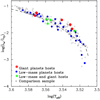 |
Fig. 1 Luminosity versus Teff for the stars analysed. Stars with gas-giant planets are shown with red filled circles, while low-mass-planet hosts are shown with blue filled circles. Stars harbouring both gas-giant and low-mass planets are shown with green stars. A 5 Gyr isochrone from Spada et al. (2013) is also shown for comparison. |
3.2 Stellar parameters and chemical abundances of the FGK primaries
We determined basic stellar parameters (Teff, log g, microturbulent velocity, and [Fe/H]) for the primary stars using the code TGVIT8 (Takeda et al. 2005) which applies the iron ionisation and excitation equilibrium conditions to a set of 302 Fe I and 28 Fe II lines. The input stellar equivalent widths (EWs) were measured automatically using the code ARES9 (Sousa et al. 2007, 2015). The reject parameter was adjusted according to the S/N of the spectra as described in Sousa et al. (2008). Uncertainties on the stellar parameters are computed by progressively changing each stellar parameter from the converged solution to a value for which one or more of the conditions (excitation equilibrium, match of the curve of growth, ionisation equilibrium) are no longer fulfilled. We note that this procedure only evaluates statistical errors (see for details Takeda et al. 2002a,b). The uncertainties due to the errors in the measurement of the EWs were also computed and added in quadrature to the ones derived by the TGVIT code. Other sources of uncertainties, such as the choice of the model atmosphere, the list lines used, or the adopted atomic parameters are not taken into account. The derived parameters are provided in Table 1.
We obtained the chemical abundances of individual elements C, O, Na, Mg, Al, Si, Ca, Sc, Ti, V, Cr, Mn, Co, Ni, and Zn using the 2017 version of the code MOOG10 (Sneden 1973) together with ATLAS9 atmosphere models (Kurucz 1993a). The used line list is given in Maldonado et al. (2015a, and references therein). Hyperfine structure (HFS) was taken into account for V I and Co I using the MOOG driver blends. Our derived abundances are provided in Table 2. They are expressed relative to the solar values derived in Maldonado et al. (2015a), using the same methodology and similar spectra. We do not consider HFS effects on Mn abundances,as Maldonado et al. (2015a) found an offset between the HFS abundances of Mn when using different lines. The uncertainties take into account the line-to-line scatter errors as well as the uncertainties due to the propagation of the errors in the stellar parameters and the equivalent widths (computed using the star HIP 116906 as reference).
Carbon abundances were derived by spectral synthesis of the CH molecular band at 430 nm using the CH line list provided in Masseron et al. (2014). These abundances are expressed relative to the solar value obtained in Baratella et al. (2020). Oxygen abundances were derived by spectral fitting of the [O I] 630 nm line. However, reliable abundances were obtained only for seven stars. Carbon and oxygen uncertainties are those due to the fitting procedure.
3.3 M dwarf abundances: methodology
In order to derive the abundances of the M stars we initially tried to proceed as in Maldonado et al. (2015b) where a large dataset of spectral features and ratios of features were identified as temperature and metallicity diagnostics. However, in spite of the fact that many of these features are found to correlate with the elemental abundances,a quick inspection of the plots of pseudo-equivalent width measurements versus [X/H] reveals flat curves or complex patterns, which are difficult to fit. Therefore, we conclude that even if the pseudo-equivalent width of a given spectroscopic feature might show a significant correlation with a specific ion abundance, the values of pseudo-equivalent widths depend on other parameters such as effective temperature, surface gravity, the global metallicity content, or the abundance of alkali metals. In addition, many of the features are likely to be a blend of different atomic or molecular lines. In other words, pseudo-equivalent-width values contain too much information to deal with.
A common technique to reduce the dimensionality of the data and find the variables in which the spread or variance of the data is larger is the so-called principal component (PCA) analysis. The PCA technique (e.g. Francis & Wills 1999) is used to extract information from correlated data sets and find a new basis on which the largest amount of variance is explained with the least number of basis vectors. This methodology has been successfully applied to samples of FGK stars even with spectroscopic data at moderate resolution (e.g. Muñoz Bermejo et al. 2013; Xiang et al. 2017; Giribaldi et al. 2019).
We initially tried to identify spectral regions sensitive to the elemental abundance of different ions. For this purpose we made use of atmospheric models together with the lists of lines used in the chemical analysis of solar-type stars and already identified spectral indexes sensitive to metallicity and other elements (e.g. Ghezzi et al. 2014). We made use of ATLAS9 models together with the spectral synthesis code SYNTHE (Kurucz 1993a,b) as it is easy to change the abundances of different elements and compute spectra with the desired abundances. We are aware that other sets of models (PHOENIX, MARCS) are usually considered to better reproduce the atmospheres of low-mass stars (e.g. Bertone et al. 2008; Sinclair et al. 2010; Maldonado 2012), but we found that better results were obtained if the full spectral range was considered (from 534 nm, to avoid the bluest region of the spectra, which suffers from a lower S/N, and the gap between the two CCDs in HARPS spectra).
Before applying the PCA, we rebinned each coadded spectrum to a common wavelength grid and smoothed to a lower resolution using a Gaussian filter of a 12 nm width. To estimate how this smoothing reduces the spectral resolution we measured the ratio λ/(δλ) on several lines in a ThAr spectra before and after the smoothing finding that it goes from ~115 000 to ~1000–2000. While it is true that smoothing and resampling the data might destroy information, it also reduces the impact of high-frequency distortion in the data, and previous works have found better results at lower resolution (Muñoz Bermejo et al. 2013). Finally, all the spectra were set to a common flux scale. In order to do this, we consider the spectral flux at the R band centred at 609 nm with only 2 nm width to avoid the inclusion of strong molecular bands. We use one of the stellar spectra as reference and perform a linear fit between the “reference” and the “problem” flux.
A flux matrix, F(n, j), was then obtained where j indexes the stars (including both the training and the problem datasets) and n is the index corresponding to the wavelength bin. Finally, PCs were computed using the available routines in the SCIKIT-LEARN python package (Pedregosa et al. 2011).
Our next step is to use the training dataset (i.e. the M dwarfs in binary systems around an FGK primary star) to find a relationship between the PCs and the stellar abundances. While some authors have explored the possibility of using a large number of PCs (e.g. Xiang et al. 2017), our training dataset is composed of only 19 stars, and so the use of a large number of PCs leads us to a reduced number of degrees of freedom. For example, a fit of the stellar abundance as a linear combination of the PCs using 17 PCs would leave us with only one degree of freedom. In order to avoid over-fitting, the use of sparse Bayesian learning algorithms has been proposed in the literature (e.g. Muñoz Bermejo et al. 2013), like the automatic relevance determination regression (ARDR).
Briefly, the target value is expected to be a linear combination of the features,
 (1)
(1)
where each coefficient wi is drawn from a Gaussian distribution centred at zero and a standard deviation αi so that
 (2)
(2)
with A = diag(α1…αp). The aim of sparse Bayesian fitting is to use the available data to compute the posterior distribution for the vector of weights w and the noise variance, σ2. Automatic relevance determination regression is based on defining the inverse variances of these Gaussian distributions, α, as variables, and to infer their values as well. Therefore, if the αi parameter of the ith feature tends to infinity, then its weight is very likely close to zero and is therefore pruned. In this way, the solution that contains the least number of non-zero elements in w is favoured, and over-fitting is avoided.
Bayesian inference proceeds by applying the Bayes rule to compute the posterior distribution over all unknowns given the data x :
 (3)
(3)
where the data, x, in our case are the PCs and the stellar abundances, P(x|w, α, σ2) is the likelihood function and gives a measure of how well the model fits the data, and P(w, α, σ2) is the prior distribution for the parameters.
The posterior in Eq. (3) cannot be computed directly; it is common to decompose it, as
 (4)
(4)
where the first term in Eq. (4) is the posterior over the weights which can be computed analytically. Therefore, the optimisation of the evidence or the learning process reduces to the maximisation of
 (5)
(5)
with respect to α and σ2. The ARDR analysis was done with the SCIKIT-LEARN python package (Pedregosa et al. 2011) where the α and σ2 hyper-parameters are assumed to follow a Gamma distribution. More details about Bayesian inference and the ARDR technique can be found in MacKay (1992); Tipping (2001) as well as on the SCIKIT-LEARN tutorials.
Initially, all 19 training stars and a total of 17 PCs were used. Stellar abundances were computed in this way for our sample of M dwarfs. The derived M dwarf metallicities were compared with a sample of nearby solar-type FGK stars coming from our previous works (Maldonado et al. 2015a). This sample was selected for comparison because the stars were analysed using similar spectra and the same methodology as for the abundances of the FGK primaries of our training M dwarfs11. We find that the derived M dwarfs metallicities are shifted towards higher values when compared with the metallicities of the nearby FGK stars. This could be related to the fact that most of our training stars have metallicities larger than −0.10 dex, while only three training stars have metallicities below this value. We discuss this issue with more detail in Sect. 3.6. To overcome this difficulty we performed a series of simulations in which 17 out of the 19 stars in the training dataset were randomly selected as training stars. For each simulation, we compared the metallicity distribution derived for our M dwarfs with the known metallicity distribution of the nearby solar-type FGK stars using a two-sample Kolmogorov-Smirnov test (hereafter KS test). We selected the “optimal” training dataset as the one that provides the most similar metallicity distribution to the one of the FGK stars. We note that to force the metallicity distribution of M dwarfs to be similar to the one of nearby FGK stars is a common practice and has been used before to derive empirical calibrations for M dwarf metallicities (e.g. Johnson & Apps 2009; Schlaufman & Laughlin 2010). It is also worth noting that instead of using all the stars included in Maldonado et al. (2015a) we restricted the comparison to FGK stars within ~70 pc (as our training stars are located within this distance) and with Galactic spatial velocity components (U, V, W) similar to the ones of the training data set. In this way we ensure that the comparison is not biased by stars located at different distances or belonging to different kinematic populations. Further, the star NLTT 15601 was discarded from the training dataset as its PCs deviate in a clear way from the values of the rest of the stars in the training dataset. We note that this star is the one with the lowest S/N of the whole training dataset.
The final number of training stars used in the computations amounts to 16 while the number of PCs is 14. In this way we use the maximum number of PCs while allowing for one degree of freedom. Figure 2 shows the comparison of the abundances derived for the training stars using our PCA technique with the abundances derived from the primaries, while the standard deviation of the differences for each element is shown in Table 3. We also show the number of training stars and PCs used aswell as the residual mean square (RMS), the root-mean squared error (RMSE), and the coefficient of determination (R2); see e.g. Appendix in Rojas-Ayala et al. (2012). We note that for Ti and Cr, whose abundances can be derived from lines of the neutral atom as well as from lines from the single ionised atom, we consider the abundances derived from lines of the neutral atom as these are more abundant than the single ionised lines. The opposite is true for Sc, and abundances from lines of the singleionised atom were considered as they are more abundant. In general, we find that the differences between ourderived abundances and those measured in the FGK primaries have standard deviation lower than ~0.10 dex, the RMS and RMSE values are close to zero, and the value of R2 is close to one, as expected when a model fit is useful for prediction. Slightly higher dispersions are found for elements like Mg, Ca, and V for which we note that their abundances are more difficult to measure even in solar-type stars. Indeed, for some stars we were not able to derive the abundances of C or Al. Therefore, for these elements we were forced to use less trainingstars and a lower number of PCs. As far as oxygen abundances are concerned, we were only able to measure theabundances in FGK primaries in six stars, and the methodology (using four PCs) fails to derive reliable values. We discuss the effect on the results of the number of training stars and PCs used in the following section.
The derived abundances for our sample of M dwarfs are given in Table A.4.
Spectroscopic properties of the primaries FGK stars.
Derived abundances and associated uncertainties ([X/H] in dex) for the primaries FGK stars.
3.4 Validation of the methodology I: comparison with FGK stars
As mentioned, we applied the PCA plus ARDR methodology to our sample of “problem” M dwarfs described in Sect. 2. Unfortunately, we do not have a sample of M dwarfs with known abundances determined from spectroscopy to validate our methodology. Some effort has been made to apply the spectral synthesis methods to M dwarfs, but to the best of our knowledge they are mainly focused on a small number of stars and mainly analyse strong atomic lines at wavelengths redder than the HARPS/HARPS-N spectral coverage (e.g. Woolf & Wallerstein 2005; Bean et al. 2006; Abia et al. 2020). Abundance analyses of M dwarfs in the near-infrared have also been performed but on a small number of stars (e.g. Önehag et al. 2012; Souto et al. 2017).
Therefore, we need to find alternative ways of testing the reliability of our methods. As a first step to validate our methodology, we compare the [X/H]-versus-[Fe/H] trends derived from our M dwarfs with those known for FGK stars, as it is reasonable to expect similar trends for both types of stars. As before, the abundance for the FGK stars came from our previous works (Maldonado et al. 2015a), although we now use the full dataset. The corresponding plots are shown in Fig. 3. Several conclusions can be drawn from this figure: good agreement between FGK and M starsis found for the abundances of C, Na, Si, Ti, Cr, Mn, and Ni, although some outliers can be seen, especially atlow and high abundance values. The [X/H]-versus-[Fe/H] relationship shows a larger spread when the abundances of Al and Zn are considered, with M dwarfs having slightly lower Zn abundances. We note that for these elements, even for solar-type stars, their abundances are based on a relatively small number of lines. For V and Ca, the general tendencies for FGK and M dwarfs are slightly different. For Mg and Sc, the tendency is similar, but M dwarfs seem to have lower abundances. The opposite is true for Co, with M dwarfs having higher abundances.
Standard deviation of the differences, residual mean square, mean squared error, and coefficient of determination between the PCA-derived abundances of the training stars and those measured in the corresponding primaries.
3.5 Validation of the methodology II: cross-validation with FGK stars
While PCA and Bayesian methods have already been used to determine stellar parameters and abundances, it is clear that the small number of training stars used in this work might raise some concern as to the applicability of these techniques. In other words, we need to be sure that sparse Bayesian methods do effectively avoid over-fitting and can be safely applied even with a small number of training stars.
We therefore performed a cross-validation of the technique, using it to derive the stellar abundances of a sample of FGK stars with HARPS/HARPS-N spectra. We use a total of 37 HARPS spectra from our previous works. Giant stars were excluded and only stars with measured abundances for all elements were considered.
A total of 100 simulations were performed. In each simulation 16 stars were randomly selected as the training dataset and exactly the same procedure as used for the M dwarfs was applied. In particular, we note that we keep the number of PCs used to 14 (as in the M dwarfs case). Figure 4 shows the results for one of the simulations, where the abundances derived from the PCA methodology are compared with the measured abundances for both the training (red circles) and problem stars (blue crosses).
We consider the standard deviation of the differences between the stellar abundances and the PCA-derived values as a measure of the goodness of the technique. For each simulation and for each element, we compute the standard deviation of the differences between the PCA–Bayes derived abundances and those derived from a curve-of-growth approach from measured EWs of selected lines in the stellar spectra (as described in Sect. 3.1). We plot the distributions of the 100 standard deviationsfrom the 100 simulation in Fig. 5. Excluding some outliers, for most elements the agreement between the PCA-derived abundances and those measured in the usual way is better than 0.10/0.15 dex. An agreement between 0.10 and 0.20 dex is found for some elements, such as Na, Mn, and Zn, whose abundances are based only on a small number of lines.
Our results show that the PCA–Bayesian fit technique can provide reliable results even if a low number of stars (as is our case) is considered in the training dataset. Certainly, a larger number of M dwarfs in the training dataset would be desirable, especially at low-abundance values. We discuss this possibility in Sect. 6.
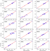 |
Fig. 2 Stellar abundances, [X/H], derived for the M dwarfs included in the training dataset using our PCA–Bayes technique versus the abundances measured in the corresponding primary stars. The red line denotes the one-to-one relationship. |
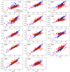 |
Fig. 3 [X/H]versus [Fe/H] for FGK stars (blue plus symbols), the M dwarf training stars (green circles), and our sample of “problem” M stars (red crosses). |
3.6 Metallicity scale of M dwarfs: comparison with previous works
We compare the metallicity values derived from the new PCA technique with those previously reported in the literature. Values for the comparison include: those values computed by us using our previous “msdlines” technique (see Sect. 2, MSDL); the metallicities provided by Rojas-Ayala et al. (2012, hereafter RA12) which are derived from spectral indexes in the near-infrared domain; the values by Önehag et al. (2012, hereafter ON12) who perform spectral synthesis in the infrared J band; those derived by Neves et al. (2013, NE13) who use a technique based on pseudo-equivalent widths of spectral features measured in optical high-resolution spectra; the values by Gaidos et al. (2014, GA14) computed from metal-sensitive atomic and molecular features; thevalues derived by Newton et al. (2014, NE14) from spectral lines and indexes in moderate-resolution near-infrared spectra; values from Woolf & Wallerstein (2020, WW20) who perform spectral synthesis in the spectral range 5700–10 000 Å; values derived by Souto et al. (2020, SO20) who perform spectral synthesis on APOGEE spectra in the H band; and values derived by Passegger et al. (2019) using stellar parameters from high-resolution spectra from spectral synthesis in both the visible wavelength range (PA19-V) and the near-infrared (PA19-N).
A comparison of iron abundances is shown in Fig. 6 while Table 4 shows the main statistics of the comparisons. The agreement is good overall in all cases with RMSE values lower than 0.10 dex (i.e. the typical uncertainties reported in M dwarf abundances).
As an additional test, in Fig. 7 we show the empirical cumulative distribution function (ECDF) of the derived metallicities compared to the metallicities of FGK stars. We also show the results if all the 19 training stars are considered as well as the ECDF obtained using the “msdlines” metallicities and the NE12 calibration. Several conclusions can be drawn from this figure: metallicity values derived from photometry (we recall that the msdlines method was calibrated using NE12 because of a lack of high-resolution spectroscopic observations of M dwarfs in binary systems around solar-type stars) provide an ECDF shifted towards lower metallicities in comparison with FGK stars for metallicity values higher than −0.20 dex. If no selection of the training dataset is performed, PCA–Bayes-derived metallicities are shifted towards higher values when compared with FGK stars. As mentioned before, this is likely a dataset shift caused by selection bias as most of our training stars have metallicities higher than +0.00 dex. Although several methods are available to deal with this problem (e.g. densityratio estimator) they have provided unsuccessful results, probably because of our reduced number of training stars. Our finally adopted metallicity values for M dwarfs do reproduce the metallicity behaviour of nearby solar-type stars. A KS test between our derived M dwarf metallicities and the FGK metallicities returns the values D = 0.04 and p-value = 0.99, with neff = 112.5, meaning that both samples show statistically identical metallicity distributions.
As a final test we checked whether our derived metallicities show any correlation with the stellar effective temperatures and masses finding no significant correlation between these quantities. For metallicity and temperature the Spearman’s rank ρ is −0.0959 ± 0.0696 with a z-score = −0.578 ± 0.422, while for metallicity and stellar mass we obtain ρ = 0.0548 ± 0.0700 and z-score = 0.329 ± 0.422. The statistical tests were performed by a bootstrap Monte Carlo (MC) simulation plus a Gaussian random shift of each data point within its error bars (Curran 2014)12. This result is expected as we derive these quantities using independent methodologies. We note that, unlike photometric calibrations,our PCA–Bayes metallicities are not based on stellar evolution models.
As far as other abundances besides iron are concerned, only a few elemental abundances for a small number of stars are available in the literature. WW20 also compute abundances of Ti, while SO20 derive abundances of C. The corresponding comparisons are shown in Fig. 8. It is clear that our derived Ti abundances are higher than those previously reported and there seems to be an offset between our derived abundances and those reported in WW20. Thereason for this offset is not clear given the good agreement between WW20 and our results for the iron abundance. For carbon, SO20 abundances are higher but the agreement is good overall and there seems to be a linear relationship between our abundances and those given in SO20. Finally, Souto et al. (2018, SO18) derived abundances of several elements (namely Fe, C, Mg, Al, Ca, and Ti) from near-infrared spectra for the star Gl 447.
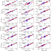 |
Fig. 4 PCA-derived abundances versus stellar abundances for our sample of FGK stars with HARPS/HARPS-N spectra from one of the performed simulations. The training dataset is shown as red circles while problem stars are shown as blue crosses. |
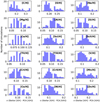 |
Fig. 5 Obtained standard deviations of the differences between the PCA-derived abundances and the measured stellar abundances for our sample of FGK stars with HARPS/-N spectra. The histograms show the results from 100 simulations. Outliers are excluded from the plot. |
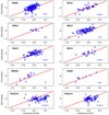 |
Fig. 6 Comparison between the iron abundances derived in this work and those previously reported in the literature. The red line denotes the one-to-one relationship. |
3.7 Stellar abundance and kinematics
Stars of the thin and thick disc populations are known to differ in terms of age, chemical composition, spatial distribution, and kinematics. Thin-disc stars rotate faster than the local standard of rest and show solar α-element abundances. On the other hand, the thick disc is enriched in α elements and lags behind the local standard of rest (e.g. Reddy et al. 2003, 2006; Bensby et al. 2014). Most of our targets have a kinematics compatible with the thin-disc population. If we consider the metallicity values derived from our PCA–Bayes analysis, we note that the mean metallicity of these stars is +0.01 dex. On the other hand, for the stars that are possible members of the thick-disc population our new technique gives a mean metallicity of −0.39 dex. As is common in the literature, we consider Mg, Si, Ca, and Ti as α elements. Whilst thin-disc stars in our sample show a mean [α/Fe] value of −0.11 dex, thick discs have larger α abundances with a mean value of +0.10 dex.
This can also be seen in Fig. 9 where we show the Toomre diagram of the observed stars. Stars are plotted with different colours and symbols according to their metallicities (left) and [α/Fe] abundances (right). The dashed lines indicate values of constant total velocities. The figure shows that low-metallicity stars span amuch larger range of total velocities than the metal-rich stars. On the other hand, stars with higher [α/Fe] abundances show larger total velocities. We conclude that our derived abundances reproduce the known kinematic trends from the different stellar populations.
Standard deviation of the differences, residual mean square, mean squared error, and coefficient of determination between the PCA-derived abundances of the training stars and those provided in previous works.
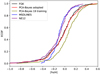 |
Fig. 7 [Fe/H] empirical cumulative distribution function for the derived metallicities with those obtained with other methods. See text for details. |
3.8 Stellar abundances and activity
In cool stars with convective outer layers, chromospheric activity and rotation are linked by the stellar dynamo (e.g. Kraft 1967; Noyes et al. 1984; Montesinos et al. 2001) and both (activity and rotation) are known to decrease with time as a star loses angular momentum with stellar winds via magnetic braking (Weber & Davis 1967; Jianke & Collier Cameron 1993). On the other hand, stellar metallicity reflects the enrichment history of the interstellar medium (e.g. Timmes et al. 1995), and for a given spectral type, young stars are expected to show higher metallicity values. In addition, stars with a greater metallicity may be more active because their convection zones tend to be deeper than those of less metallic stars with the same parameters and because the chromospheric emission in metal spectral lines may be enhanced (cf. Karoff et al. 2018). We caution thatthis result has been observed in only one solar twin star, and so similar analyses on other stars are needed for confirmation. In particular, it is unclear whether it would also hold for low-mass stars, and especially for fully convective late-M dwarfs.
We tested whether this is the case. Activity indexes in the main optical indicators, Ca II H and K, Balmer lines (from Hα to Hɛ), Na I, D1, D2, and He I D3 were computed following the bandpasses defined in Maldonado et al. (2019a). Figure 10 shows the mean Ca II (left) and Hα (right) activity index values of the stars divided into three metallicity bins as a function of spectral type. When considering the calcium index the figure clearly shows a tendency for higher levels of activity at higher metallicities for a given spectral type, which suggests that stars with higher activity have higher metallicities. For Hα, the tendency is even more clear. Similar results are obtained for the other activity indexes (not shown). Our conclusion is that our derived abundances reproduce the expected trends with stellar activity.
4 Completeness of the planet host sample
Our aim is to understand planet formation and evolution as a function of the main stellar properties. It is therefore fundamental to our analysis to select stars for which planets of a given mass and period can be detected in a uniform way. In order to estimate the detectability limits of our planet hosts, we proceeded as in Maldonado et al. (2019b). For each star we collected all the available HARPS and HARPS-N data. We are aware that for many stars there should be radial velocities measured with other instruments. However, given that radial-velocity time series are usually not available for non-planet detections, we decided to focus only on HARPS and HARPS-/N data. This is certainly a conservative approach, as it might overestimate the detection limits for some periods. However, it is a robust and homogeneous method and allows us to obtain an efficient determination of the detection limits. More detailed detection limits around samples of M dwarfs, in particular for the stars included in the HADES survey, will be addressed in forthcoming studies.
For each star, radial velocities were computed from the available data using the TERRA pipeline (Anglada-Escudé & Butler 2012), which provides a better radial-velocity accuracy when applied to M dwarfs (Perger et al. 2017). For those stars with known planets, we used the code rvlin13 (Wright & Howard 2009) to subtract the contribution of the planets to the radial velocity using a multiplanet Keplerian fit with the planetary periods fixed to the published values.
We then computed the expected radial-velocity semi-amplitude due to the presence of different types of planets by sampling in logarithmic space the planetary mass–period space. In particular, planetary masses from 0.005 to 80 MJup and orbital periods from 1 to 104 days were considered. Circular orbits were considered, as it has been shown that planet detection limits are not strongly dependent on eccentricity (Endl et al. 2002; Cumming & Dragomir 2010). For each planet, the expected radial velocities were computed keeping the same time as in the original observations. Several realisations of the radial velocity were performed, each one corresponding to a different phase offset. Following previous works (Galland et al. 2005; Lagrange et al. 2012; Meunier et al. 2012), we consider a planet as detectable around a given star if the root mean square (rms) of the planet’s expected radial velocity is larger than the rms of the residuals of the stellar radial velocity (i.e. after subtracting the signals of the already known planets) in each of the simulated phases.
The derived detection probability curves are shown in Fig. 11. For each period, the curves show the percentage of stars from our sample for which planets with corresponding minimum mass can be detected. The results show that for ~80% of the stars in our sample, low-mass planets within a ten-day period might be detected. Gaseous planets more massive than 100 M⊕ and ~200 M⊕ with periods within 100 and 1000 days, respectively, can also be excluded for ~80% of the stars. It can be seen that several known planets are actually located under the 2% probability curve. This is not surprising; as mentioned before our approach is relatively conservative.
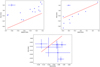 |
Fig. 8 Comparison between our PCA–Bayes-derived abundances and those reported by WW20 (Ti, top left panel), SO20 (C, top right panel), and SO18 (Fe, C, Mg, Al, Ca, and Ti for the star Gl 447, bottom panel). The red line denotes the one-to-one relationship. |
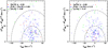 |
Fig. 9 Toomre diagram for the stars analysed in this work. Stars are shown with different colours and symbols according to their iron abundances (left) and [α/Fe] abundances (right). Intervals in [Fe/H] and [α/Fe] were selected to show the stars in the Q10 and Q90 quartiles of the distribution. |
5 Results
Our sample is composed of a total of 204 stars with homogeneous mass and metallicity measurements. Five stars host at least one giant planet (hereafter giant-host subsample), while 29 stars harbour at least one low-mass planet (hereafter low-mass host subsample). Two stars, namely GJ 15A and Gl 433, host at least one low-mass planet (Gl 433 hosts two) plus an additional planet somehow in the boundary between low-mass and giant (minimum masses 36 and 32 M⊕, respectively). These two stars were considered in the low-mass planet subsample. On the other hand, Gl 832 and Gl 876 harbour low-mass companions as well as planets more massive than 200 M⊕, and so we add these stars to the giant-host subsample. As seen before, given the available data, it is unlikely that stars in the low-mass host and comparison subsamples host a non-detected gas-giant planet at short periods (with the data at hand, they should already have been detected). However, we cannot rule out the possibility that stars in the comparison subsample host non-detected low-mass planets. In the following, unless otherwise noted, we consider the stellar metallicity values derived with the PCA–Bayes technique.
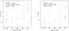 |
Fig. 10 Ca II H and K (left) and Hα (right) activity indexes as a function of spectral sub-type. Mean values for stars in three bins of metallicity are shown with different colours. |
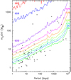 |
Fig. 11 Minimum mass vs. planetary period. Substellar companions known around M dwarfs are shown as grey circles. Detection probability curves are superimposed with different colours. The horizontal dashed line indicates the standard mass loci of low-mass planets and gas-giant planet companions. |
5.1 Biases
Before we proceed further in the comparison between the different subsamples, an exploration of the possible sources of bias that could mimic metallicity differences is called for. To this end, we compared the different subsamples in terms of distance, age, and kinematics, which are the parameters most likely to affect the metal content of a star. The comparison is given in Table 5, while Fig. 12 shows the corresponding cumulative distribution functions for the distance (left), age (centre), and the Toomre diagram (right).
The comparison shows that while there seems to be no differences in terms of age or kinematics between planet hosts and the comparison stars, stars with planets tend to be systematically located at shorter distances. We note that typical uncertainties in the stellar age are of around 4 Gyr, while errors on the distance are of around 0.03 pc. A KS test confirms that there are no differences in terms of age (D = 0.24, p-value = 0.18, neff = 18.94 for comparison/low-mass hosts; and D = 0.36, p-value = 0.43, neff = 5.75 for comparison/giant hosts), while low-mass planet hosts are located at shorter distances (D = 0.41, p-value = 0.0002, neff = 26.1 for comparison/low-mass hosts; and D = 0.28, p-value = 0.59, neff = 6.7 for comparison/giant hosts). This trend could reflect a bias in the exoplanet surveys, as closer stars are usually brighter and thus higher-S/N observations can be obtained with shorter integration times. Therefore, closer and brighter stars can beobserved with a more dense temporal cadence and higher S/N values, thus favouring the detection of planets.
Comparison between the properties of the different samples analysed in this work.
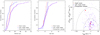 |
Fig. 12 Cumulative distribution function for the distance (left), age (centre), and Toomre diagram (right) for the stars analysed in this work. |
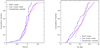 |
Fig. 13 [Fe/H] (left) and stellar mass (right) cumulative distributions for the different samples studied in this work. |
5.2 Metallicity distribution
The cumulative distribution function of the metallicity for the different samples analysed in this work is presented inthe left panel of Fig. 13. For guidance, some statistical diagnostics are also given in Table 6. The figure shows a tendency of giant hosts to show high metallicities although their cumulative distribution does not appear to be very different from those of the comparison sample. On the other hand, the low-mass hosts also show a similar metallicity distribution to the comparison sample. A KS test shows that there are no statistically significant differences between the metallicity distributions of the three subsamples (D = 0.21, p-value = 0.16, and neff = 26.1 for comparison/low-mass hosts; and D = 0.25, p-value = 0.70, and neff = 6.7 for comparison/giant hosts).
Figure 13 shows that M dwarfs with gas-giant planets might have high metallicity values (suggesting that the gas-giant planet–metallicity correlation found on FGK stars might also hold for M dwarfs) although the trend requires statistical confirmation. On the other hand, stars with low-mass planets do not show the metal-rich signature. These results seem to be in line with previous works (Bonfils et al. 2007; Johnson & Apps 2009; Schlaufman & Laughlin 2010; Rojas-Ayala et al. 2012; Terrien et al. 2012; Neves et al. 2013).
The left panel of Fig. 14 shows the fraction of gas-giant planets (light orange) and low-mass planets (light blue) as a function of stellar metallicity. The errors in the frequency of each bin are calculated using the binomial distribution,
 (6)
(6)
where P(fp, n, N) is the probability of n detections given a sample of size N when the true planetary companion frequency is fp. Given that the probability distribution is not symmetric about its maximum, a common practice is to report the range in planetary fraction that delimits 68.2% of the integrated probability function, which is equivalent to the 1σ limits for a Gaussian distribution (e.g. Burgasser et al. 2003; Endl et al. 2006; Sozzetti et al. 2009; Neves et al. 2013).
The fraction of stars with planets was fitted to a function with the functional form f = C10α[Fe/H], following previous works (e.g. Fischer & Valenti 2005; Udry & Santos 2007), although other functional forms have been discussed in the literature (e.g. Mortier et al. 2013). Our analysis provides C = 0.20 ± 0.03 and α = −0.12 ± 0.16 for the low-mass planets hosts; and C = 0.04 ± 0.02 and α = 0.98 ± 0.87 for the giant hosts.
Two conclusions can be drawn from this analysis. First, the frequency of low-mass planets does not seem to be a function of the stellar metallicity. Furthermore, as the α value is negative there might be an anti-correlation, that is, a decreasing fraction of planet frequency with increasing stellar metallicity. This result seems to be in line with previous analyses of samples of M dwarfs (Neves et al. 2013). Second, gas-giant planets show a planet–metallicity correlation with an α value compatible within errors with the values found for FGK stars, namely ~1.7 (e.g. Fischer & Valenti 2005). However, our value of α is lower than previous values found in samples of M dwarfs, namely of α ~1.26–2.94 (Neves et al. 2013). Nevertheless, we caution that the uncertainty on α is high, and we have not taken into account a possible dependence of the planet fraction on stellar mass. We address these issues in the following sections.
[Fe/H] statistics of the stellar samples.
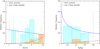 |
Fig. 14 Fraction of gas-giant planets (light orange) and low-mass planets (light blue) as a function of the stellar [Fe/H] (left) and stellar mass (right). The best bin fitting is shown in red for gas-giant planets and in blue for low-mass planets. |
5.3 Mass distribution
Planet occurrence is also known to show a dependence on stellar mass (Laws et al. 2003; Lovis & Mayor 2007; Johnson et al. 2007, 2010a). The right panel of Fig. 13 shows the cumulative distribution function of the stellar mass for the samples analysed in this work. Planet hosts appear to be less massive than the comparison stars, although this could be an observational bias, as planets are easier to find around less massive stars. Some statistical diagnostics are also provided in Table 7. The results from a KS tests provide D = 0.20, p-value = 0.19, and neff = 26.1 for comparison/low-mass hosts; and D = 0.26, p-value = 0.69, and neff = 6.7 for comparison/giant hosts.
The right panel of Fig. 14 shows the fraction of gas-giant planets (light orange) and low-mass planets (light blue) as a function of stellar mass. The fraction of stars with planets was fitted to a power-law function  as previous works have shown that planet occurrence rises monotonically with stellar mass (Johnson et al. 2010a). The derived values are C = 0.06 ± 0.06 and α = 0.94 ± 1.23 for the gas-giant-planet hosts; and C = 0.18 ± 0.05 and α = −0.41 ± 0.25 for the low-mass-planet hosts.
Our results show that gas-giant planet occurrence increases with stellar mass in line with previous findings (Johnson et al. 2010a; Montet et al. 2014), while the frequency of low-mass planets tends to decrease as we move towards more massive stars. This last finding might be subject to observational bias due to the fact that small planets are easier to detect around less-massive stars. However, we note that a similar trend, that is, a higher frequency of planets towards less massive stars has been found in the Kepler data (Hardegree-Ullman et al. 2019).
Stellar mass statistics of the stellar samples.
5.4 Simultaneous fit to stellar mass and metallicity
Finally, we test planet frequency as a function of stellar mass and metallicity simultaneously. For this purpose, we followed a Bayesian approach, discussed at length in Johnson et al. (2010a), Mortier et al. (2013), and Montet et al. (2014).
Briefly, we fit the planetary frequency as a function of the mass and metallicity through the following relationship:
 (7)
(7)
where M is the stellar mass, F is the stellar metallicity, and X = (C, α, β) are the parameters to be optimised. Each star represents a Bernoulli trial and the probability of finding a planet at a given mass and metallicity is given by the binomial distribution. For a total of T stars, the probability of a detection around a star i (of H total detections) is given by f(Mi, Fi), while the probability of a non-detection around a star j is 1 − f(Mj, Fj). The probability of a specific model X, considering our data d, is given by the Bayes theorem:
![\begin{equation*}P(X\vert d) \propto P(X) \prod_{i}^{H} f(M_{i}, F_{i}) \times \prod_{j}^{T-H} {[}1-f(M_{j}, F_{j}){]}. \end{equation*}](/articles/aa/full_html/2020/12/aa39478-20/aa39478-20-eq9.png) (8)
(8)
The mass and metallicity of each star are considered to follow a Gaussian distribution with means (Mi, Fi) and standard deviations (σM,i, σF,i), and so the predicted planet fraction for the ith star is:
 (9)
(9)
The marginal log likelihood is finally obtained by taking logarithms in Eq. (8):
![\begin{eqnarray*} \mathcal{L}&\equiv&\log P(X/d)\propto\sum_{i}^{H}\log f(M_{i},F_{i})+ \sum_{j}^{T-H}\log[1-f(M_{j},F_{j})] \nonumber \\ &&+\log P(X). \end{eqnarray*}](/articles/aa/full_html/2020/12/aa39478-20/aa39478-20-eq11.png) (10)
(10)
Our results are shown in Table 8 where the median values and their corresponding 68.2% confidence interval are provided, while Fig. 15 shows the marginal posterior probability distribution functions for the model parameters for the gas-giant planets (left) and for low-mass planets (right). Uniform distribution priors were chosen for the parameters.
Table 9 shows a comparison between the results from this work and those previously reported in the literature. Our results are consistent with a planet–metallicity correlation for gas-giant planets. We find that the dependence of the gas-giant planet frequency on stellar metallicity, β = 1.28, is lower than what is known for FGK stars but is compatible within errors; that is, the frequency of gas-giant planets goes as ~102[Fe/H]. In particular we note that our result is fully compatible with the findings of Johnson et al. (2010a), based on an analysis of FGKM stars including intermediate-mass subgiants. However, our results suggest a weaker gas-giant-planet–metallicity correlation than that found in recent works focusing on M dwarfs, which found a dependency on metallicity with β values of between 2 and 4 (Neves et al. 2013; Montet et al. 2014). We also find a stronger dependence of the gas-giant planet frequency on stellar mass, α = 1.77, than recent works. That is, we find a slightly weaker gas-giant-planet–metallicity correlation in M dwarfs, but a stronger planet–stellar mass correlation, and so it is possible that lower metallicity environments can be compensated by a higher stellar (and therefore disc) mass, allowing gas-giant-planet formation to occur. This is consistent with the view that the mass of solids in protoplanetary discs is the main factor controlling the formation of planets and can be explained in the framework of core-accretion models (e.g. Pollack et al. 1996; Ida & Lin 2004; Mordasini et al. 2009, 2012).
Regarding low-mass planets, their frequency does not seem to depend on the stellar mass (in disagreement with what we find in the bin fitting). We confirm that the frequency of low-mass planets does not depend on, or might show an anti-correlation with, increasing stellar metallicity.
As the value of β derived here is lower than the values obtained by other works focusing on M dwarfs, we repeated our analysis, this time using the metallicities obtained by the msdlines code. The results are C = 0.07 , α = 1.65
 , and β = 3.94
 for the gas-giant hosts, and C = 0.09
 , α = 0.22
 , and β = –1.13
 when considering the low-mass planet-host subsample. The corresponding posterior distributions are shown in Fig. 16. It can be seen that the values of the parameter α obtained using the msdlinesmetallicities are similar to the one obtained using the PCA–Bayes values for the low-mass-planet sample. On the contrary, the value of β differs. The value obtained using the PCA–Bayes metallicities is compatible with a rather flat dependency of the low-mass planet frequency on stellar metallicity. However, the value obtained when using the msdlines metallicities (β = –1.13) might indicate an anti-correlation.
On the other hand, for the gas-giant sample we obtain a similar mass dependency, but a clearly stronger correlation between planet occurrence and stellar metallicity. This is in line with the works of Neves et al. (2013) and Montet et al. (2014) who find that M dwarfs should show a stronger giant-planet–metallicity correlation than their FGK counterparts given their smaller protoplanetary disc masses. We caution that the posterior distributions of the parameters α and β are very broad and their associated uncertainties very high. This could be related to the small size of the giant-host subsample.
Given that the msdlines metallicities are shifted towards lower values when compared with the nearby FGK stars (see Fig. 7) we speculate whether the very high β values found in previous works (~3, 4) and with our msdlines metallicities may be related to the use of a photometric scale. However, further analysis is required to clarify this issue.
Parameters of the Bayesian fit.
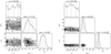 |
Fig. 15 Marginal posterior probability distribution functions of the fit to Eq. (7) for gas-giant planets (left), and for low-mass planets (right). The metallicity values used in this analysis are those derived with the PCA–Bayes technique developed in this work. |
Comparison with previous works.
5.5 Other chemical signatures
To try to find differences in the abundances of other chemical elements besides iron, we show in Fig. 17 the cumulative distribution of the [X/H] abundances of the comparison M dwarfs, the low-mass-planet hosts, and the giant-planet-host subsamples. Some statistical diagnostics are shown in Table 10, where the results of a KS test for each element are also listed.
Similar behaviour between planet and non-planet hosts is found for all element abundances, both for gas-giant and low-mass planets. However, slightly higher abundances of Ti, Na, Mg, and Al can be seen for gas-giant-planet hosts. Slightly lower abundances of Co for low-mass-planet hosts can also be seen. As these trends are not statistically significant we conclude that our results are similar to those for FGK stars where planet hosts have been shown to have abundances that are indiscernible from those of stars without planets (e.g. Bodaghee et al. 2003; Ecuvillon et al. 2006; Gonzalez 2006; Gilli et al. 2006; da Silva et al. 2011; Adibekyan et al. 2012a). We included the α abundance in our analysis as Adibekyan et al. (2012b,a) showed that planet-hosting stars with low-metallicity values tend to belong to the thick disc and show high α values, but besides the general trend of higher α abundances in less-metallic stars discussed in Sect. 3.7, no differences in α abundances were found between planet hosts and non-planet hosts. It is important to note that chemical differences between planet hosts and non-planet hosts, when claimed, are relatively modest. For instance, a depletion of only ~0.08 dex in refractory elements relative to volatile elements has been found in the Sun and other solar analogues (e.g. Meléndez et al. 2009; Ramírez et al. 2009). In Table 3 we list the standard deviation of the differences between the PCA-derived abundances and those measured in the corresponding primaries for our training dataset. These values can be considered as a lower limit on the uncertainties derived. It is clear that we are still far from achieving the same precision in abundance analyses as that obtained for FGK stars, and so small chemical differences beyond the limits of our precision could still be present in our sample.
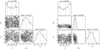 |
Fig. 16 Marginal posterior probability distribution functions of the fit to Eq. (7) for gas-giant planets (left) and for low-mass planets (right). The metallicity values used in this analysis are those derived with the msdlines code. |
Comparison between the elemental abundances of the different subsamples.
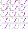 |
Fig. 17 [X/H] cumulative fraction of low-mass-planet hosts (blue), gas-giant-planet hosts (red), and comparison M dwarfs (purple). |
6 Conclusions
M dwarfs are considered to be promising targets in the search for small, rocky, potentially habitable planets. They also constitute valuable tools for understanding planet formation as a function of stellar mass. However, analysis of their optical spectra has proven to be a difficult task. In this work, we develop a technique to derive stellar abundances of M dwarfs from the same optical, high-resolution spectra that are used in exoplanet searches, that is, without relying on additional infrared observations or atmosphericmodels.
Our methodology is based on the use of a PCA and Bayesian regression methods. The procedure is trained with spectra of M dwarfs orbiting around an FGK primary. We find the agreement between the abundances derived using our method and those measured in the FGK primary to be better than 0.10 dex in most cases. While it is true that these dispersions should be regarded as lower limits on the uncertainties of our technique, we believe that it is encouraging to see that they are of the same order of magnitude as the dispersion found in the individual abundances of FGK stars when measured from different lines of the same ion. A cross-validation of the technique performed on FGK stellar spectra shows that in spite of the small training sample used, the methodology seems to provide reliable abundances.
As we are lacking a suitable comparison sample, we are forced to compare our derived abundances for M dwarfs with the known trends for FGK stars. We find similar [X/H]-versus-[Fe/H] trends for M dwarfs and FGK stars for most of the ions. We also show that our PCA–Bayes metallicities reproduce the metallicity scale of nearby FGK stars. On the contrary, metallicity values derived from photometry provide a ECDF distribution shifted towards lower metallicities in comparison with FGK stars. Nevertheless, we recognise that the methodology can be improved by observing more training stars. This is specially evident at low metallicities. Further observations of M dwarfs in the near-infrared domain will help us to validate our techniques.
To the best of our knowledge, we present the first detailed chemical analysis of several elements for a large sample of M dwarfs with and without surrounding gas-giant and low-mass planets. We note that while it is unlikely that giant planets are hidden in the sample, we cannot discard the possibility that there are more non-detected low-mass planets in the different subsamples analysed in this work. A comparison of the properties of the different subsamples reveals no differences in age or kinematics between planet hosts and non-planet hosts. We find planet hosts to be located at lower distances than the comparison sample. This likely reveals the fact that closer stars are brighter and easier to observe at higher S/N.
Regarding the dependency of the planetary fraction on stellar metallicity and mass, our results confirm the findings of previous works. That is, the frequency of gas-giant planets is a function of the host star metallicity as well as a function of the host star mass. However, we note that our PCA–Bayes metallicities predict a weaker planet–metallicity correlation and a stronger mass dependency than photometric values for giant-planet hosts. On the other hand, the frequency of low-mass planets around M dwarfs is not a function of stellar metallicity, although a weak anti-correlation might be present. We also find an anti-correlation between the frequency of low-mass planets around M dwarfs and stellar mass in line with recent results from the Kepler mission. However, we caution that this anti-correlation is found only in the bin-fitting analysis, but not in the Bayesian fit. For other elements besides iron, we do not find differences in the abundance distributions of stars with and without planets. These results are in line with what is known from the chemical analysis of solar-type stars and can be explained within the framework of core-accretion models.
We finally note that the homogeneous determination of stellar abundances of M dwarfs might be of interest for many other studies dealing withthe local properties of the Galaxy, for example the study of stars in clusters and other stellar associations. Our codes are public available14 for the benefit of the whole community.
Acknowledgements
This research was supported by the Italian Ministry of Education, University, and Research through the PREMIALEWOW 2013 research project under grant Ricerca di pianeti intorno a stelle di piccola massa. J.M. acknowledges support from the Accordo Attuativo ASI-INAF n. 2018.22.HH.O, Partecipazione alla fase B1 della missione Ariel (ref. G. Micela). M.P., I.R., J.C.M, and E.H acknowledge support from the Spanish Ministry of Science and Innovation and the European Regional Development Fund through grant PGC2018-098153-B- C33, as well as the support of the Generalitat de Catalunya/CERCA programme. J.I.G.H. acknowledges financial support from Spanish Ministry of Science and Innovation (MICINN) under the 2013 Ramón y Cajal program RYC-2013-14875. A.S.M. acknowledges financial support from the Spanish MICINN under the 2019 Juan de la Cierva Programme. B.T.P. acknowledges Fundación La Caixa for the financial support received in the form of a Ph.D. contract. J.I.G.H., R.R., A.S.M., B.T.P. acknowledge financial support from the Spanish MICINN AYA2017-86389-P. This research has made use of the NASA Exoplanet Archive, which is operated by the California Institute of Technology, under contract with the National Aeronautics and Space Administration under the Exoplanet Exploration Program. This work has made use of data from the European Space Agency (ESA) mission Gaia (https://www.cosmos.esa.int/gaia), processed by the Gaia Data Processing and Analysis Consortium (DPAC, https://www.cosmos.esa.int/web/gaia/dpac/consortium). Funding for the DPAC has been provided by national institutions, in particular the institutions participating in the Gaia Multilateral Agreement. Additional data collected at the European Southern Observatory and Telescopio Nazionale Galileo under programme ID GAPS, 082.C-0718(B), 072.C-0488(E), 183.C-0437(A), 180.C-0886(A), 198.C-0838(A), 0101.C-0516(A), 1102.C-0339(A), 183.C-0972(A), 096.C-0460(A), 082.C-0718(A), 191.C-0505(A), 096.C-0499(A), 191.C-0873, 191.C-0873(A), 088.C-0662(B), 089.C-0497(A), 090.C-0395(A), 087.C-0831(A), 093.C-0409(A), 60.A-9036(A), 192.C-0224(G), 192.C-0224(H), 192.C-0224(C), CAT14B_162, CAT16A_99, 198.C-0873(A), CAT17A_95, CAT14A_43, OPT16A_11, CAT16A_134, 092.C-0721(A), 0100.C-0097(A), 0101.C-0379(A), 0102.C-0558(A), CAT13B_170, CAT14A_128, 185.D-0056(A), 185.D-0056(B), 185.D-0056(K), 076.C-0155(A), 086.C-0284(A), 089.C-0732(A), 090.C-0421(A), 0101.D-0494(A), 192.C-0224(B), 099.C-0205(A), 085.C-0019(A), 495.L-0963(A), 097.C-0390(B), 099.C-0798(A), 0100.C-0487(A), 0101.D-0494(B), 095.C-0718(A), 077.C-0364(E), 097.C-0864(B), 099.C-0880(A), 075.C-0202(A), 192.C-0224, 098.C-0739(A), 60.A-9709(G), 060.A-9709(G), 074.C-0364(A), 078.C-0044(A), 097.C-0561(A), 075.D-0614(A), have been used. We sincerely appreciate the careful reading of the manuscript and the constructive comments of the anonymous referee.
References
- Abia, C., Tabernero, H. M., Korotin, S. A., et al. 2020, A&A, 642, A227 [CrossRef] [EDP Sciences] [Google Scholar]
- Adibekyan, V. Z., Santos, N. C., Sousa, S. G., et al. 2012a, A&A, 543, A89 [NASA ADS] [CrossRef] [EDP Sciences] [Google Scholar]
- Adibekyan, V. Z., Delgado Mena, E., Sousa, S. G., et al. 2012b, A&A, 547, A36 [NASA ADS] [CrossRef] [EDP Sciences] [Google Scholar]
- Adibekyan, V. Z., González Hernández, J. I., Delgado Mena, E., et al. 2014, A&A, 564, L15 [NASA ADS] [CrossRef] [EDP Sciences] [Google Scholar]
- Affer, L., Micela, G., Damasso, M., et al. 2016, A&A, 593, A117 [NASA ADS] [CrossRef] [EDP Sciences] [Google Scholar]
- Anglada-Escudé, G., & Butler, R. P. 2012, ApJS, 200, 15 [NASA ADS] [CrossRef] [Google Scholar]
- Antoniadis-Karnavas, A., Sousa, S. G., Delgado-Mena, E., et al. 2020, A&A, 636, A9 [CrossRef] [EDP Sciences] [Google Scholar]
- Baratella, M., D’Orazi, V., Biazzo, K., et al. 2020, A&A, 640, A123 [CrossRef] [EDP Sciences] [Google Scholar]
- Bean, J. L., Benedict, G. F., & Endl, M. 2006, ApJ, 653, L65 [NASA ADS] [CrossRef] [Google Scholar]
- Bensby, T., Feltzing, S., & Lundström, I. 2003, A&A, 410, 527 [NASA ADS] [CrossRef] [EDP Sciences] [Google Scholar]
- Bensby, T., Feltzing, S., Lundström, I., & Ilyin, I. 2005, A&A, 433, 185 [NASA ADS] [CrossRef] [EDP Sciences] [Google Scholar]
- Bensby, T., Feltzing, S., & Oey, M. S. 2014, A&A, 562, A71 [NASA ADS] [CrossRef] [EDP Sciences] [Google Scholar]
- Bertone, E., Buzzoni, A., Chávez, M., & Rodríguez-Merino, L. H. 2008, A&A, 485, 823 [NASA ADS] [CrossRef] [EDP Sciences] [Google Scholar]
- Bodaghee, A., Santos, N. C., Israelian, G., & Mayor, M. 2003, A&A, 404, 715 [NASA ADS] [CrossRef] [EDP Sciences] [Google Scholar]
- Bonfils, X., Mayor, M., Delfosse, X., et al. 2007, A&A, 474, 293 [NASA ADS] [CrossRef] [EDP Sciences] [Google Scholar]
- Bonfils, X., Delfosse, X., Udry, S., et al. 2013, A&A, 549, A109 [NASA ADS] [CrossRef] [EDP Sciences] [Google Scholar]
- Buchhave, L. A., Latham, D. W., Johansen, A., et al. 2012, Nature, 486, 375 [NASA ADS] [Google Scholar]
- Burgasser, A. J., Kirkpatrick, J. D., Reid, I. N., et al. 2003, ApJ, 586, 512 [NASA ADS] [CrossRef] [Google Scholar]
- Butler, R. P., Johnson, J. A., Marcy, G. W., et al. 2006, PASP, 118, 1685 [NASA ADS] [CrossRef] [Google Scholar]
- Carpenter, J. M. 2001, AJ, 121, 2851 [NASA ADS] [CrossRef] [Google Scholar]
- Cosentino, R., Lovis, C., Pepe, F., et al. 2012, SPIE Conf. Ser., 8446, 84461V [Google Scholar]
- Courcol, B., Bouchy, F., & Deleuil, M. 2016, MNRAS, 461, 1841 [NASA ADS] [CrossRef] [Google Scholar]
- Cumming, A., & Dragomir, D. 2010, MNRAS, 401, 1029 [NASA ADS] [CrossRef] [Google Scholar]
- Cumming, A., Butler, R. P., Marcy, G. W., et al. 2008, PASP, 120, 531 [CrossRef] [Google Scholar]
- Curran, P. A. 2014, ArXiv e-prints [arXiv:1411.3816] [Google Scholar]
- Cutri, R. M., Skrutskie, M. F., van Dyk, S., et al. 2003, VizieR Online Data Catalog: II/246 [Google Scholar]
- da Silva, R., Milone, A. C., & Reddy, B. E. 2011, A&A, 526, A71 [NASA ADS] [CrossRef] [EDP Sciences] [Google Scholar]
- Dressing, C. D., & Charbonneau, D. 2013, ApJ, 767, 95 [NASA ADS] [CrossRef] [Google Scholar]
- Ecuvillon, A., Israelian, G., Santos, N. C., et al. 2006, A&A, 445, 633 [NASA ADS] [CrossRef] [EDP Sciences] [Google Scholar]
- Endl, M., Kürster, M., Els, S., et al. 2002, A&A, 392, 671 [NASA ADS] [CrossRef] [EDP Sciences] [Google Scholar]
- Endl, M., Cochran, W. D., Tull, R. G., & MacQueen, P. J. 2003, AJ, 126, 3099 [NASA ADS] [CrossRef] [Google Scholar]
- Endl, M., Cochran, W. D., Kürster, M., et al. 2006, ApJ, 649, 436 [Google Scholar]
- Fischer, D. A., & Valenti, J. 2005, ApJ, 622, 1102 [NASA ADS] [CrossRef] [Google Scholar]
- Francis, P. J., & Wills, B. J. 1999, ASP Conf. Ser., 162, 363 [Google Scholar]
- Gaia Collaboration (Brown, A. G. A., et al.) 2018, A&A, 616, A1 [NASA ADS] [CrossRef] [EDP Sciences] [Google Scholar]
- Gaidos, E., Mann, A. W., Lépine, S., et al. 2014, MNRAS, 443, 2561 [NASA ADS] [CrossRef] [Google Scholar]
- Galland, F., Lagrange, A. M., Udry, S., et al. 2005, A&A, 443, 337 [NASA ADS] [CrossRef] [EDP Sciences] [Google Scholar]
- Ghezzi, L., Cunha, K., Smith, V. V., et al. 2010, ApJ, 720, 1290 [NASA ADS] [CrossRef] [Google Scholar]
- Ghezzi, L., Dutra-Ferreira, L., Lorenzo-Oliveira, D., et al. 2014, AJ, 148, 105 [NASA ADS] [CrossRef] [Google Scholar]
- Gilli, G., Israelian, G., Ecuvillon, A., Santos, N. C., & Mayor, M. 2006, A&A, 449, 723 [NASA ADS] [CrossRef] [EDP Sciences] [Google Scholar]
- Giribaldi, R. E., Porto de Mello, G. F., Lorenzo-Oliveira, D., Amôres, E. B., & Ubaldo-Melo, M. L. 2019, A&A, 629, A33 [CrossRef] [EDP Sciences] [Google Scholar]
- Gonzalez, G. 1997, MNRAS, 285, 403 [NASA ADS] [CrossRef] [Google Scholar]
- Gonzalez, G. 2006, PASP, 118, 1494 [NASA ADS] [CrossRef] [Google Scholar]
- González Hernández, J. I., Israelian, G., Santos, N. C., et al. 2010, ApJ, 720, 1592 [NASA ADS] [CrossRef] [Google Scholar]
- González Hernández, J. I., Delgado-Mena, E., Sousa, S. G., et al. 2013, A&A, 552, A6 [NASA ADS] [CrossRef] [EDP Sciences] [Google Scholar]
- Hardegree-Ullman, K. K., Cushing, M. C., Muirhead, P. S., & Christiansen, J. L. 2019, AJ, 158, 75 [NASA ADS] [CrossRef] [Google Scholar]
- Henry, T. J., & McCarthy, D. W., J. 1993, AJ, 106, 773 [NASA ADS] [CrossRef] [Google Scholar]
- Howard, A. W., Marcy, G. W., Bryson, S. T., et al. 2012, ApJS, 201, 15 [NASA ADS] [CrossRef] [Google Scholar]
- Hubickyj, O., Bodenheimer, P., & Lissauer, J. J. 2005, Icarus, 179, 415 [NASA ADS] [CrossRef] [Google Scholar]
- Ida, S., & Lin, D. N. C. 2004, ApJ, 616, 567 [NASA ADS] [CrossRef] [MathSciNet] [Google Scholar]
- Jianke, L., & Collier Cameron, A. 1993, MNRAS, 261, 766 [NASA ADS] [CrossRef] [Google Scholar]
- Johnson, J. A., & Apps, K. 2009, ApJ, 699, 933 [NASA ADS] [CrossRef] [Google Scholar]
- Johnson, D. R. H., & Soderblom, D. R. 1987, AJ, 93, 864 [NASA ADS] [CrossRef] [Google Scholar]
- Johnson, J. A., Butler, R. P., Marcy, G. W., et al. 2007, ApJ, 670, 833 [NASA ADS] [CrossRef] [Google Scholar]
- Johnson, J. A., Aller, K. M., Howard, A. W., & Crepp, J. R. 2010a, PASP, 122, 905 [NASA ADS] [CrossRef] [Google Scholar]
- Johnson, J. A., Howard, A. W., Marcy, G. W., et al. 2010b, PASP, 122, 149 [NASA ADS] [Google Scholar]
- Karoff, C., Metcalfe, T. S., Santos, Â. R. G., et al. 2018, ApJ, 852, 46 [NASA ADS] [CrossRef] [Google Scholar]
- Kim, Y.-C., Demarque, P., Yi, S. K., & Alexander, D. R. 2002, ApJS, 143, 499 [NASA ADS] [CrossRef] [Google Scholar]
- Kraft, R. P. 1967, ApJ, 150, 551 [NASA ADS] [CrossRef] [Google Scholar]
- Kurucz, R. 1993a, ATLAS9 Stellar Atmosphere Programs and 2 km/s grid. Kurucz CD-ROM No. 13 (Cambridge, MA: Smithsonian Astrophysical Observatory), 1993, 13 [Google Scholar]
- Kurucz, R. 1993b, SYNTHE Spectrum Synthesis Programs and Line Data, Kurucz CD-ROM No. 18. (Cambridge, MA: Smithsonian Astrophysical Observatory), 18 [Google Scholar]
- Lagrange, A. M., De Bondt, K., Meunier, N., et al. 2012, A&A, 542, A18 [NASA ADS] [CrossRef] [EDP Sciences] [Google Scholar]
- Laws, C., Gonzalez, G., Walker, K. M., et al. 2003, AJ, 125, 2664 [NASA ADS] [CrossRef] [Google Scholar]
- Lovis, C., & Mayor, M. 2007, A&A, 472, 657 [NASA ADS] [CrossRef] [EDP Sciences] [Google Scholar]
- MacKay, D. J. C. 1992, Neural Comput., 4, 415 [CrossRef] [Google Scholar]
- Maldonado, J. 2012, PhD thesis, Universidad Autónoma de Madrid, Spain [Google Scholar]
- Maldonado, J., & Villaver, E. 2016, A&A, 588, A98 [NASA ADS] [CrossRef] [EDP Sciences] [Google Scholar]
- Maldonado, J., Eiroa, C., Villaver, E., Montesinos, B., & Mora, A. 2015a, A&A, 579, A20 [NASA ADS] [CrossRef] [EDP Sciences] [Google Scholar]
- Maldonado, J., Affer, L., Micela, G., et al. 2015b, A&A, 577, A132 [NASA ADS] [CrossRef] [EDP Sciences] [Google Scholar]
- Maldonado, J., Phillips, D. F., Dumusque, X., et al. 2019a, A&A, 627, A118 [NASA ADS] [CrossRef] [EDP Sciences] [Google Scholar]
- Maldonado, J., Villaver, E., Eiroa, C., & Micela, G. 2019b, A&A, 624, A94 [CrossRef] [EDP Sciences] [Google Scholar]
- Mann, A. W., Gaidos, E., & Ansdell, M. 2013a, ApJ, 779, 188 [NASA ADS] [CrossRef] [Google Scholar]
- Mann, A. W., Brewer, J. M., Gaidos, E., Lépine, S., & Hilton, E. J. 2013b, AJ, 145, 52 [NASA ADS] [CrossRef] [Google Scholar]
- Masseron, T., Plez, B., Van Eck, S., et al. 2014, A&A, 571, A47 [NASA ADS] [CrossRef] [EDP Sciences] [Google Scholar]
- Mayor, M., & Queloz, D. 1995, Nature, 378, 355 [Google Scholar]
- Mayor, M., Pepe, F., Queloz, D., et al. 2003, The Messenger, 114, 20 [NASA ADS] [Google Scholar]
- Mayor, M., Marmier, M., Lovis, C., et al. 2011, ArXiv e-prints [arXiv:1109.2497] [Google Scholar]
- Meléndez, J., Asplund, M., Gustafsson, B., & Yong, D. 2009, ApJ, 704, L66 [NASA ADS] [CrossRef] [Google Scholar]
- Meunier, N., Lagrange, A. M., & De Bondt, K. 2012, A&A, 545, A87 [NASA ADS] [CrossRef] [EDP Sciences] [Google Scholar]
- Montes, D., López-Santiago, J., Gálvez, M. C., et al. 2001, MNRAS, 328, 45 [NASA ADS] [CrossRef] [MathSciNet] [Google Scholar]
- Montes, D., González-Peinado, R., Tabernero, H. M., et al. 2018, MNRAS, 479, 1332 [Google Scholar]
- Montesinos, B., Thomas, J. H., Ventura, P., & Mazzitelli, I. 2001, MNRAS, 326, 877 [NASA ADS] [CrossRef] [Google Scholar]
- Montet, B. T., Crepp, J. R., Johnson, J. A., Howard, A. W., & Marcy, G. W. 2014, ApJ, 781, 28 [NASA ADS] [CrossRef] [Google Scholar]
- Mordasini, C., Alibert, Y., & Benz, W. 2009, A&A, 501, 1139 [NASA ADS] [CrossRef] [EDP Sciences] [Google Scholar]
- Mordasini, C., Alibert, Y., Benz, W., Klahr, H., & Henning, T. 2012, A&A, 541, A97 [NASA ADS] [CrossRef] [EDP Sciences] [Google Scholar]
- Mortier, A., Santos, N. C., Sousa, S., et al. 2013, A&A, 551, A112 [NASA ADS] [CrossRef] [EDP Sciences] [Google Scholar]
- Muñoz Bermejo, J., Asensio Ramos, A., & Allende Prieto, C. 2013, A&A, 553, A95 [NASA ADS] [CrossRef] [EDP Sciences] [Google Scholar]
- Mulders, G. D., Pascucci, I., & Apai, D. 2015a, ApJ, 798, 112 [Google Scholar]
- Mulders, G. D., Pascucci, I., & Apai, D. 2015b, ApJ, 814, 130 [NASA ADS] [CrossRef] [Google Scholar]
- Neves, V., Bonfils, X., Santos, N. C., et al. 2012, A&A, 538, A25 [NASA ADS] [CrossRef] [EDP Sciences] [Google Scholar]
- Neves, V., Bonfils, X., Santos, N. C., et al. 2013, A&A, 551, A36 [NASA ADS] [CrossRef] [EDP Sciences] [Google Scholar]
- Neves, V., Bonfils, X., Santos, N. C., et al. 2014, A&A, 568, A121 [NASA ADS] [CrossRef] [EDP Sciences] [Google Scholar]
- Newton, E. R., Charbonneau, D., Irwin, J., et al. 2014, AJ, 147, 20 [NASA ADS] [CrossRef] [Google Scholar]
- Noyes, R. W., Hartmann, L. W., Baliunas, S. L., Duncan, D. K., & Vaughan, A. H. 1984, ApJ, 279, 763 [NASA ADS] [CrossRef] [Google Scholar]
- Önehag, A., Heiter, U., Gustafsson, B., et al. 2012, A&A, 542, A33 [NASA ADS] [CrossRef] [EDP Sciences] [Google Scholar]
- Passegger, V. M., Reiners, A., Jeffers, S. V., et al. 2018, A&A, 615, A6 [NASA ADS] [CrossRef] [EDP Sciences] [Google Scholar]
- Passegger, V. M., Schweitzer, A., Shulyak, D., et al. 2019, A&A, 627, A161 [NASA ADS] [CrossRef] [EDP Sciences] [Google Scholar]
- Pedregosa, F., Varoquaux, G., Gramfort, A., et al. 2011, J. Mach. Learn. Res., 12, 2825 [Google Scholar]
- Perger, M., García-Piquer, A., Ribas, I., et al. 2017, A&A, 598, A26 [NASA ADS] [CrossRef] [EDP Sciences] [Google Scholar]
- Perryman, M. 2018, The Exoplanet Handbook (Cambridge: Cambridge University Press) [CrossRef] [Google Scholar]
- Pinamonti, M., Sozzetti, A., Giacobbe, P., et al. 2019, A&A, 625, A126 [CrossRef] [EDP Sciences] [Google Scholar]
- Pollack, J. B., Hubickyj, O., Bodenheimer, P., et al. 1996, Icarus, 124, 62 [NASA ADS] [CrossRef] [Google Scholar]
- Quirrenbach, A., Amado, P. J., Ribas, I., et al. 2018, SPIE Conf. Ser., 10702, 107020W [Google Scholar]
- Ramírez, I., Meléndez, J., & Asplund, M. 2009, A&A, 508, L17 [NASA ADS] [CrossRef] [EDP Sciences] [Google Scholar]
- Ramírez, I., Meléndez, J., Bean, J., et al. 2014, A&A, 572, A48 [NASA ADS] [CrossRef] [EDP Sciences] [Google Scholar]
- Rauscher, E., & Marcy, G. W. 2006, PASP, 118, 617 [NASA ADS] [CrossRef] [Google Scholar]
- Reddy, B. E., Tomkin, J., Lambert, D. L., & Allende Prieto, C. 2003, MNRAS, 340, 304 [NASA ADS] [CrossRef] [Google Scholar]
- Reddy, B. E., Lambert, D. L., & Allende Prieto, C. 2006, MNRAS, 367, 1329 [NASA ADS] [CrossRef] [Google Scholar]
- Rojas-Ayala, B., Covey, K. R., Muirhead, P. S., & Lloyd, J. P. 2012, ApJ, 748, 93 [NASA ADS] [CrossRef] [Google Scholar]
- Santos, N. C., Israelian, G., & Mayor, M. 2004, A&A, 415, 1153 [NASA ADS] [CrossRef] [EDP Sciences] [Google Scholar]
- Schlaufman, K. C., & Laughlin, G. 2010, A&A, 519, A105 [NASA ADS] [CrossRef] [EDP Sciences] [Google Scholar]
- Schweitzer, A., Passegger, V. M., Cifuentes, C., et al. 2019, A&A, 625, A68 [NASA ADS] [CrossRef] [EDP Sciences] [Google Scholar]
- Sinclair, J. A., Helling, C., & Greaves, J. S. 2010, MNRAS, 409, L49 [NASA ADS] [Google Scholar]
- Sneden, C. A. 1973, PhD thesis, The University of Texas at Austin, Austin, USA [Google Scholar]
- Soubiran, C., Jasniewicz, G., Chemin, L., et al. 2018, A&A, 616, A7 [NASA ADS] [CrossRef] [EDP Sciences] [Google Scholar]
- Sousa, S. G., Santos, N. C., Israelian, G., Mayor, M., & Monteiro, M. J. P. F. G. 2007, A&A, 469, 783 [NASA ADS] [CrossRef] [EDP Sciences] [Google Scholar]
- Sousa, S. G., Santos, N. C., Mayor, M., et al. 2008, A&A, 487, 373 [NASA ADS] [CrossRef] [EDP Sciences] [MathSciNet] [Google Scholar]
- Sousa, S. G., Santos, N. C., Israelian, G., Mayor, M., & Udry, S. 2011, A&A, 533, A141 [NASA ADS] [CrossRef] [EDP Sciences] [Google Scholar]
- Sousa, S. G., Santos, N. C., Adibekyan, V., Delgado-Mena, E., & Israelian, G. 2015, A&A, 577, A67 [NASA ADS] [CrossRef] [EDP Sciences] [Google Scholar]
- Souto, D., Cunha, K., García-Hernández, D. A., et al. 2017, ApJ, 835, 239 [NASA ADS] [CrossRef] [Google Scholar]
- Souto, D., Unterborn, C. T., Smith, V. V., et al. 2018, ApJ, 860, L15 [NASA ADS] [CrossRef] [Google Scholar]
- Souto, D., Cunha, K., Smith, V. V., et al. 2020, ApJ, 890, 133 [CrossRef] [Google Scholar]
- Sozzetti, A., Torres, G., Latham, D. W., et al. 2009, ApJ, 697, 544 [NASA ADS] [CrossRef] [Google Scholar]
- Spada, F., Demarque, P., Kim, Y. C., & Sills, A. 2013, ApJ, 776, 87 [NASA ADS] [CrossRef] [Google Scholar]
- Takeda, Y., Ohkubo, M., & Sadakane, K. 2002a, PASJ, 54, 451 [NASA ADS] [CrossRef] [Google Scholar]
- Takeda, Y., Sato, B., Kambe, E., Sadakane, K., & Ohkubo, M. 2002b, PASJ, 54, 1041 [NASA ADS] [Google Scholar]
- Takeda, Y., Ohkubo, M., Sato, B., Kambe, E., & Sadakane, K. 2005, PASJ, 57, 27 [NASA ADS] [CrossRef] [Google Scholar]
- Terrien, R. C., Mahadevan, S., Bender, C. F., et al. 2012, ApJ, 747, L38 [NASA ADS] [CrossRef] [Google Scholar]
- Timmes, F. X., Woosley, S. E., & Weaver, T. A. 1995, ApJS, 98, 617 [NASA ADS] [CrossRef] [Google Scholar]
- Tipping, M. E. 2001, J. Mach. Learn. Res., 1, 211 [Google Scholar]
- Udry, S., & Santos, N. C. 2007, ARA&A, 45, 397 [NASA ADS] [CrossRef] [Google Scholar]
- Weber, E. J., & Davis, L., J. 1967, ApJ, 148, 217 [NASA ADS] [CrossRef] [Google Scholar]
- Wolszczan, A., & Frail, D. A. 1992, Nature, 355, 145 [NASA ADS] [CrossRef] [Google Scholar]
- Woolf, V. M., & Wallerstein, G. 2005, MNRAS, 356, 963 [NASA ADS] [CrossRef] [Google Scholar]
- Woolf, V. M., & Wallerstein, G. 2020, MNRAS, 494, 2718 [CrossRef] [Google Scholar]
- Wright, J. T., & Howard, A. W. 2009, ApJS, 182, 205 [NASA ADS] [CrossRef] [Google Scholar]
- Xiang, M. S., Liu, X. W., Shi, J. R., et al. 2017, MNRAS, 464, 3657 [CrossRef] [Google Scholar]
- Yi, S., Demarque, P., Kim, Y.-C., et al. 2001, ApJS, 136, 417 [NASA ADS] [CrossRef] [Google Scholar]
See e.g. http://exoplanet.eu/ or http://exoplanets.org/
With the only exception of the carbon abundances, which in Maldonado et al. (2015a) were derived from atomic lines.
All Tables
Derived abundances and associated uncertainties ([X/H] in dex) for the primaries FGK stars.
Standard deviation of the differences, residual mean square, mean squared error, and coefficient of determination between the PCA-derived abundances of the training stars and those measured in the corresponding primaries.
Standard deviation of the differences, residual mean square, mean squared error, and coefficient of determination between the PCA-derived abundances of the training stars and those provided in previous works.
Comparison between the properties of the different samples analysed in this work.
All Figures
|
Fig. 1 Luminosity versus Teff for the stars analysed. Stars with gas-giant planets are shown with red filled circles, while low-mass-planet hosts are shown with blue filled circles. Stars harbouring both gas-giant and low-mass planets are shown with green stars. A 5 Gyr isochrone from Spada et al. (2013) is also shown for comparison. |
| In the text | |
|
Fig. 2 Stellar abundances, [X/H], derived for the M dwarfs included in the training dataset using our PCA–Bayes technique versus the abundances measured in the corresponding primary stars. The red line denotes the one-to-one relationship. |
| In the text | |
|
Fig. 3 [X/H]versus [Fe/H] for FGK stars (blue plus symbols), the M dwarf training stars (green circles), and our sample of “problem” M stars (red crosses). |
| In the text | |
|
Fig. 4 PCA-derived abundances versus stellar abundances for our sample of FGK stars with HARPS/HARPS-N spectra from one of the performed simulations. The training dataset is shown as red circles while problem stars are shown as blue crosses. |
| In the text | |
|
Fig. 5 Obtained standard deviations of the differences between the PCA-derived abundances and the measured stellar abundances for our sample of FGK stars with HARPS/-N spectra. The histograms show the results from 100 simulations. Outliers are excluded from the plot. |
| In the text | |
|
Fig. 6 Comparison between the iron abundances derived in this work and those previously reported in the literature. The red line denotes the one-to-one relationship. |
| In the text | |
|
Fig. 7 [Fe/H] empirical cumulative distribution function for the derived metallicities with those obtained with other methods. See text for details. |
| In the text | |
|
Fig. 8 Comparison between our PCA–Bayes-derived abundances and those reported by WW20 (Ti, top left panel), SO20 (C, top right panel), and SO18 (Fe, C, Mg, Al, Ca, and Ti for the star Gl 447, bottom panel). The red line denotes the one-to-one relationship. |
| In the text | |
|
Fig. 9 Toomre diagram for the stars analysed in this work. Stars are shown with different colours and symbols according to their iron abundances (left) and [α/Fe] abundances (right). Intervals in [Fe/H] and [α/Fe] were selected to show the stars in the Q10 and Q90 quartiles of the distribution. |
| In the text | |
|
Fig. 10 Ca II H and K (left) and Hα (right) activity indexes as a function of spectral sub-type. Mean values for stars in three bins of metallicity are shown with different colours. |
| In the text | |
|
Fig. 11 Minimum mass vs. planetary period. Substellar companions known around M dwarfs are shown as grey circles. Detection probability curves are superimposed with different colours. The horizontal dashed line indicates the standard mass loci of low-mass planets and gas-giant planet companions. |
| In the text | |
|
Fig. 12 Cumulative distribution function for the distance (left), age (centre), and Toomre diagram (right) for the stars analysed in this work. |
| In the text | |
|
Fig. 13 [Fe/H] (left) and stellar mass (right) cumulative distributions for the different samples studied in this work. |
| In the text | |
|
Fig. 14 Fraction of gas-giant planets (light orange) and low-mass planets (light blue) as a function of the stellar [Fe/H] (left) and stellar mass (right). The best bin fitting is shown in red for gas-giant planets and in blue for low-mass planets. |
| In the text | |
|
Fig. 15 Marginal posterior probability distribution functions of the fit to Eq. (7) for gas-giant planets (left), and for low-mass planets (right). The metallicity values used in this analysis are those derived with the PCA–Bayes technique developed in this work. |
| In the text | |
|
Fig. 16 Marginal posterior probability distribution functions of the fit to Eq. (7) for gas-giant planets (left) and for low-mass planets (right). The metallicity values used in this analysis are those derived with the msdlines code. |
| In the text | |
|
Fig. 17 [X/H] cumulative fraction of low-mass-planet hosts (blue), gas-giant-planet hosts (red), and comparison M dwarfs (purple). |
| In the text | |
Current usage metrics show cumulative count of Article Views (full-text article views including HTML views, PDF and ePub downloads, according to the available data) and Abstracts Views on Vision4Press platform.
Data correspond to usage on the plateform after 2015. The current usage metrics is available 48-96 hours after online publication and is updated daily on week days.
Initial download of the metrics may take a while.