| Issue |
A&A
Volume 643, November 2020
|
|
|---|---|---|
| Article Number | A11 | |
| Number of page(s) | 9 | |
| Section | Planets and planetary systems | |
| DOI | https://doi.org/10.1051/0004-6361/202039038 | |
| Published online | 27 October 2020 | |
Transit timing variation signature of planet migration: the case of K2-24
naXys, Department of Mathematics, University of Namur,
Rempart de la Vierge 8,
5000
Namur, Belgium
e-mail: jean.teyssandier@unamur.be
Received:
26
July
2020
Accepted:
9
September
2020
The convergent migration of two planets in a gaseous disc can lead to mean motion resonance (MMR) capture. In addition, pairs of planets in or near MMRs are known to produce strong transit timing variations (TTVs). In this paper, we study the impact of disc-induced migrations on the TTV signal of pairs of planets that enter a resonant configuration. We show that disc-induced migration creates a correlation between the amplitude and the period of the TTVs. We study the case of K2-24, a system of two planets whose period ratio indicates that they are in or near the 2:1 MMR, with non-zero eccentricities and large-amplitude TTVs. We show that a simple disc-induced migration cannot reproduce the observed TTVs. Moreover, we propose a formation scenario in which the capture in resonance during migration in a disc with strong eccentricity damping is followed by eccentricity excitation during the dispersal of the disc. This is assisted by a third planet whose presence has been suggested by radial velocity observations. This scenario accounts for the eccentricities of the two planets and their period ratio, and it accurately reproduces the amplitude and period of the TTVs. It allows for a unified view of the formation and evolution history of K2-24, from disc-induced migration to its currently observed properties.
Key words: celestial mechanics / protoplanetary disks / planet–disk interactions / planets and satellites: formation / planets and satellites: dynamical evolution and stability / planets and satellites: detection
© ESO 2020
1 Introduction
Pairs of adjacent planets in the Kepler catalogue that are close to a mean motion resonance (MMR) are often found to be exterior to the exact commensurability1, with a dearth of planets interior to it (Fabrycky et al. 2014). The fact that pairs of planets can be found in or near an MMR is not a surprise: convergent migration of two planets in a disc is known to be able to trap them in an MMR (see, e.g., Snellgrove et al. 2001; Lee & Peale 2002), and the ratio of their orbital periods is expected to be very close to the exact commensurability. However, the fact that these pairs of planets are often found on one side of the exact commensurability is considered more surprising.
Several studies (e.g. Novak et al. 2003; Papaloizou & Terquem 2010; Lithwick & Wu 2012; Batygin & Morbidelli 2013; Delisle & Laskar 2014) have argued that tides raised on the planets can cause a resonant repulsion of the two planets, hereby slightly increasing their period ratios and explaining the trend seen in the Kepler data. Other mechanisms have been proposed that also favour planet pairs lying just outside of exact commensurabilities: in-situ growth of planets via planetesimal accretion (Petrovich et al. 2013), or interactions with a planetesimal disc (Chatterjee & Ford 2015).
However, it is worth noting that one should not expect resonant pairs to be observed exactly at the precise commensurability. Precession of the orbits tends to shift the centre of the resonance away from its exact commensurability. For convergent migration, this offset can naturally produce pairs of planets with period ratios larger than the exact commensurability (see e.g. Ramos et al. 2017; Terquem & Papaloizou 2019).
In parallel to their period ratio distribution, systems near MMRs have also drawn a lot attention due to the significant transit timing variations (TTVs) they often produce. These variations result from perturbations (in general gravitational perturbations from other planets), which modify the periodicity at which a planet transits in front of its parent star. In addition to being able to reveal or confirm the presence of non-transiting planets (Miralda-Escudé 2002; Schneider 2004; Agol et al. 2005; Holman & Murray 2005; Cochran et al. 2011; Ford et al. 2012; Steffen et al. 2012), TTVs provide a way of inferring masses and eccentricities in multiple-transiting systems (Nesvorný & Morbidelli 2008; Lithwick et al. 2012; Hadden & Lithwick 2017). In particular, systems near MMRs are subject to large TTV signals (see e.g. Lithwick et al. 2012). The amplitude and period of the TTV signal depends strongly on the distance to the exact commensurability, and on the eccentricities of the planets. These quantities are often shaped during the planet-disc interaction phase.
Since disc migration can produce planets in or near MMRs (a process that tends to excite their eccentricities), and since these quantities play a key role in TTVs of planet pairs, it is natural to ask what the effect of disc migration on TTV signals is. This is the goal of this work. We focus on the K2-24 system, for which Petigura et al. (2018) obtained accurate periods, masses, and TTVs, and managed to estimate the eccentricities. In Sect. 2, we review in more detail why K2-24 is a good laboratory to test the impact of planet migration on TTVs. In Sect. 3, we carry out numerical simulations to study the TTV signals for pairs of planets that have migrated in a disc. We then suggest that an additional mechanism involving a third planet and an evaporating disc can explain the current architecture of the K2-24 system (Sect. 4). Finally, we discuss the implications of our results in Sect. 5 and conclude in Sect. 6.
2 Generalities
2.1 Properties of K2-24
The planetary system K2-24 was first reported by Petigura et al. (2016), with subsequent refined measurements by Dai et al. (2016), Sinukoff et al. (2016), Crossfield et al. (2016), and Mayo et al. (2018). The latest data for this system wereprovided by Petigura et al. (2018), who conducted a joint TTV and radial velocity (RV) analysis, which allowed them to better constrain the masses and orbits of K2-24b and c. We summarise their main findings below.
The K2-24 system has at least two planets (referred to as b and c), with masses of mb = 19 M⊕, mc = 15 M⊕, and periods of 20.89 and 42.34 days (period ratio of 2.028), around a star with a mass of M* = 1.07 M⊙. The system is thus near the 2:1 MMR and shows strong TTVs. The eccentricities of the two known planets are non-zeros. In particular, RV data only ruled out high eccentricity orbits, giving upper limits of eb < 0.39 and ec < 0.34. On the other hand, TTV data gave a constraint on a linear combination of masses and eccentricities. Using RV data to break the mass degeneracy, Petigura et al. (2018) managed to get a range of eb and ec consistent with their joint RV/TTV analysis (see their Fig. 7). In an attempt to better constrain the eccentricities, Petigura et al. (2018) assumed K2-24 to be part of the population of TTV-active Kepler multi-planet systems, and used a Rayleigh eccentricity distribution with ⟨e⟩ = 0.03 as a prior (see e.g. Wu & Lithwick 2013). From that they deduced the eccentricities of K2-24b and c to be around 0.07. It is worth noting that relaxing this assumption allows for best fits with eccentricities in the range of 0.1–0.2 (see Fig. 7 of Petigura et al. 2018). The two key features of the TTV signal are its amplitude of about 0.25 and 0.5 days for planets b and c, respectively, and its period of ~1580 days.
In addition, Petigura et al. (2018) reported the possible detection of K2-24d, a third planet with a mass of  and semi-major axis of
  . In order to understand why the specific characteristics of K2-24 are at odds with a simple model of disc migration, it is useful to first review the theory behind TTV signals near resonances, which we do in the next section.
2.2 Theory of TTVs
Transit timing variations have long been recognised as a powerful technique to detect unseen planets in systems with at least one transiting planet, and to better constrain masses and eccentricities (Miralda-Escudé 2002; Agol et al. 2005; Holman & Murray 2005; Agol & Fabrycky 2018).
As previously mentioned, K2-24b and c exhibit large amplitude TTVs, with a period of ~1580 days. In order to use these TTV measurements as a constraint on the system’s formation and dynamical history, it is useful to review the basis of the theory of TTVs. In particular, Lithwick et al. (2012) developed an analytical model for two planets near a first-order MMR, as is the case for K2-24, which is near the 2:1 resonance. We summarise the main results of this analysis here.
Firstly, we focus on the period of the TTV signal. We consider two planets near the 2:1 MMR with orbital periods P1 and P2 such as P1 < P2, and masses m1 and m2. We define the normalised distance to the exact commensurability as
 (1)
(1)
Close to an MMR, Steffen (2006) and Lithwick et al. (2012) showed that the TTV signal undergoes periodic cycles on a period given by the “super-period”  , whose value depends on the distance to the exact commensurability:
 (2)
(2)
For K2-24, we have Δ = 0.0134 and  .
.
Now we consider the amplitude of the TTV. Lithwick et al. (2012) showed that the key quantity to consider is the free eccentricity of the planets. For a planet with eccentricity e and argument of pericentre ϖ, it is convenient to introduce the complex eccentricity z = eexp(iϖ). The complex eccentricity can be decomposed into two terms, a free eccentricity zfree, and a forced eccentricity zforced (see e.g. Murray & Dermott 1999):
 (3)
(3)
The forced eccentricity arises from the resonant perturbations and is determined by the planets’ proximity to exact commensurability, while the free eccentricity is unrelated to the resonance. Near the 2:1 resonance, Lithwick et al. (2012) showed that, to leading order in eccentricity, the forced eccentricity can be expressed as:
 (4)
(4)
Here, μi = mi∕M*, and λ = 2λ2 − λ1 is the longitude of conjunctions (λ1 and λ2 being the mean longitudes). In addition, f and g are coefficients that represent the secular and resonant coupling of the two planets. They can be found in Table 3 of Lithwick et al. (2012). Near the 2:1 resonance, they read f = −1.19 + 2.20Δ and g = 0.4284 − 3.69Δ, at first order in Δ. The main result of the analysis conducted by Lithwick et al. (2012) is that the key quantity in determining the amplitude of the TTV signal is a linear combination of the free complex eccentricity of each planet:
 (5)
(5)
Lithwick et al. (2012) showed that the amplitude of the TTVs of each planet increases linearly with |Zfree∕Δ|. The TTV analysis of Petigura et al. (2018), in synergy with their RV measurements, gave the following constraints for Zfree in K2-24:
 (6)
(6)
As previously stated, Petigura et al. (2018) then assumed a prior on the eccentricity distribution (a Rayleigh distribution parametrised by a mean eccentricity ⟨e⟩ = 0.03) and deducedthat e1 ~ 0.06 and e2 ≲ 0.07. However, if one relaxes the assumption that the eccentricities in K2-24 follow such Rayleigh distribution, the only strong constraint on the eccentricities is given by Eq. (6). The contour of eccentricities allowed by the joint RV-TTV analysis can be seen in Fig. 7 of Petigura et al. (2018). Apart from the fact that none of the eccentricities are zero, we are left with a wide range of possible eccentricities for K2-24b and c.
2.3 Departure from exact commensurability
Now that we hold a good understanding of the TTV signal near the 2:1 resonance, we need to focus on the values of Δ (i.e. how far are they from the exact commensurability?) that are expected from convergent disc migration.
The two resonant angles of a system in a 2:1 MMR are (see e.g. Murray & Dermott 1999)
 (7)
(7)
We consider a resonant state in which θ1 and θ2 librate and their time derivatives average to zero. In addition, without exterior perturbation, the two planets are locked in common apsidal precession, so that  . Setting
  to zero, we arrive at
 (8)
(8)
where n1 and n2 are the mean motions. Near the 2:1 resonance, at the lowest order in eccentricity, ϖ1 varies as (Murray & Dermott 1999):
 (9)
(9)
where f1 can be expressed as Laplace coefficients, and takes the value f1 ≃−1.19 for α = a1∕a2 = 2−2∕3. Finally (in the most common case where θ1 librates around 0; see e.g. Lee 2004), Eq. (8) can be re-written:
 (10)
(10)
where Δ is defined in Eq. (1). A similar result was derived by Ramos et al. (2017). Hence, the smaller the eccentricity, the further from exact commensurability (i.e. P2∕P1 = 2) a system will be.
Resonant migration causes eccentricities to grow, a process that is balanced by eccentricity damping from the disc, leading to an equilibrium eccentricity. The equilibrium eccentricity depends on the eccentricity and semi-major-axis damping times, and therefore on the disc parameters. The general formula for the equilibrium eccentricities of two planets undergoing convergent migration with different eccentricity and semi-major-axis damping timescales can be found in Terquem & Papaloizou (2019). In the case of the 2:1 resonance, they analytically derived the equilibrium eccentricity of the inner planet as
 (11)
(11)
where i = 1, 2 labels the planets with increasing distance from the star, and τe,i, τa,i, ai, and mi are the eccentricity damping time, semi-major-axis damping time, semi-major axis, and mass of planet i, respectively.Hence, for a given pair of planets and a given set of damping times, one can use Eqs. (10) and (11) to predict the departure from exact commensurability.
2.4 Constraints and puzzles
For the sake of discussion, in this section we assume the eccentricities of ~ 0.07 quoted by Petigura et al. (2018) for K2-24b and c. We see later on that the eccentricities are likely to be higher than that, which would only make our argument stronger. Assuming that the masses that we observe now for the two planets are the same masses they had when entering the resonance, Eq. (10) suggests that in order to achieve P2 ∕P1 = 2.028 (the observed period ratio of K2-24), the equilibrium eccentricity reached by e1 during migration is 0.0024, which is a factor 30 lower than the eccentricity currently observed. At least two scenarios can resolve this discrepancy.
Scenario 1
The eccentricity and migration damping times are such that e1 managed to grow to 0.06 during disc migration. According to Eq. (10), the system should therefore have reached a period ratio of P2 ∕P1 ≃ 2.001 during the migration, a ratio significantly lower than what is observed. A subsequent mechanism is then required to push the planets further apart until they reach their current period ratio.
Scenario 2
The eccentricity and migration damping times are such that the system naturally settles at a configuration where P2 ∕P1 = 2.028 during migration. The eccentricities are smaller than what is observed today, and a subsequent mechanism is required to increase them to their current values. In the first scenario, a mechanism is required to push the planets away from the exact commensurability. One such mechanism is tidal interaction with the star (see e.g. Lithwick & Wu 2012). Since tidal forces quickly become negligible as the distance to the star increases, it is thought that this mechanism only applies to planets with periods of 10 to 20 days, putting K2-24b at the limit of validity of this mechanism. More importantly, tidal interactions would damp the eccentricities, and therefore cannot be reconciled with the non-zero eccentricities of K2-24. Another mechanism involves interactions of the pair of planets with a disc of planetesimals (Chatterjee & Ford 2015). The mechanism also leads to damping of eccentricity of the planets here, and therefore does not apply to K2-24.
In the second scenario, the current period ratio is achieved during disc migrations, but eccentricities still need to be excited. This is the scenario we focus on in the remainder of the paper. The convergent migration of the pair of planets to their current period ratio is discussed in Sect. 3, while the excitation of the planetary eccentricities is the subject of Sect. 4.
3 Formation of the resonant pair during disc migration
3.1 Planet migration
We simulated planet migration in a disc using N-body simulations. The equations of motion of each planet are modified to account for radial migration and eccentricity damping (see, e.g., Papaloizou & Larwood 2000). Namely, damping of the semi-major axis (on a timescale τa) and eccentricity (on a timescale τe) are obtained by adding the following acceleration:
 (12)
(12)
where ri (i = 1, 2) is the position vector of the ith planet (we note that the second term on the right-hand side also gives rise to a small semi-major-axis damping of order e2 ∕τe; see e.g. Teyssandier & Terquem 2014).
3.2 Disc model
In order to simulate the migration of the two planets in the disc, we need to adopt some values for the migration and damping timescales τa and τe, as introduced in Sect. 3.1. In general, these timescales depend on the disc and planet properties. In particular, given the masses of K2-24b and c, they are unlikely to be in the gap-opening (i.e. Type II) migration regime. However, some of the timescale formulas derived for Earth-mass planets in the Type I migration regime may not apply either.
In this work, we closely followed the model of Kanagawa et al. (2018) and Kanagawa & Szuszkiewicz (2020), since it applies to the range of planetary masses we are considering.
We considered a disc whose surface density Σ is given by a power-law:
 (13)
(13)
We adopted a small flaring for the disc’s scale height, thus the disc aspect ratio h is given by:
 (14)
(14)
The disc viscosity is represented by the classical α parametrisation, and we assume that α is constant throughout the disc.
The torque exerted by the disc on the planet can be scaled by the following quantity:
 (15)
(15)
where ΩK is the Keplerian frequency. Adopting a locally isothermal disc model, the Lindblad and corotation torques normalised by Γ0 and denoted γL and γC, respectively, are as follows:

Here, β = −2f + 1 and b = 0.4hp∕ɛ, where hp is the disc’s aspect ratio at the location of the planet rp, and ɛ is a softening length for the planetary gravitational potential, which is taken to be 0.6 times the disc’s scale height at the location of the planet.
Finally, the simulations of Kanagawa et al. (2018) indicate that the torque exerted by the disc on the planet is proportional to the surface density at the bottom of the gap created by the planet, rather than the unperturbed surface density. Several studies (e.g. Duffell & MacFadyen 2013; Fung et al. 2014; Kanagawa et al. 2015) have shown that the depth of the gap is controlled by the following parameter:
 (18)
(18)
With the parameters that we consider in this paper, we have K ~ 100 and a marginal gap can be opened, putting us in an intermediate regime between the pure Type I and Type II migration regimes.
Equipped with all these definitions, we can now give the expression for the semi-major-axis damping time derived by Kanagawa et al. (2018) as:
 (19)
(19)
where Kt = 20 represents the gap depth for which the corotation torque becomes ineffective. The coefficient τ0 is defined by:
 (20)
(20)
The eccentricity damping time is taken to be proportional to τa :
 (21)
(21)
where Ce is a coefficient representing uncertainties in the eccentricity damping mechanism. In the linear theory of low-mass planets, Tanaka & Ward (2004) found Ce = 1.28. However, hydrodynamical simulations have found stronger eccentricity damping than what is suggestedby the linear theory (see e.g. Cresswell & Nelson 2006, who suggested dividing Ce by 10 to better match their hydrodynamical simulations).
In order to halt migration at the observed location of K2-24b and c, we assumed that once planet b reaches ab = 0.16 au, all damping times start increasing with time at a rate of exp(t∕tslow). Once ab reaches 0.1518, the simulation stops. Several mechanisms have been studied to halt the migration at the inner edge of protoplanetary discs, which rely on the intricate physics of wave reflection and torque saturation near the inner edge (Tanaka et al. 2002; Masset et al. 2006; Tsang 2011; Miranda & Lai 2018). Our simple prescription gives an ideal representation of these complicated mechanisms.
3.3 Simulation outcomes
In this section, we present the result of 300 N-body simulations of planets, with the accelerations given in Eq. (12) added as extra forces. Simulations were carried out using the REBOUND code (Rein & Liu 2012). In Table 1, we give the list of parameters that we varied and the range of values that we chose to explore for these parameters.
Convergent migration of the two planets is a necessary condition for them to be captured in resonance. This requires τa,2 < τa,1. In practice, we find that this condition is satisfied for discs with surface density index s = 0.5 or s = 1, h = 0.025 to 0.035, and α = 0.001 to 0.005. We assume that the disc has a flaring index of f = 1∕4. The disc’s surface density coefficient, Σ0, is computed using the disc’s mass and assuming that the disc extends from 0.25 to 50 au. The timescale for slowing down migration at the inner edge is tslow = 104 yr. Both planets are initially on circular and coplanar orbits. Once had drawn the initial semi-major axis of the inner planet, we noted the semi-major axis of the second planet as 1.8 times larger. The planetary masses are fixed to the ones of K2-24b and c.
In Fig. 1, we show an example of two planets ending up with final periods of 20.87 and 42.31 days (period ratio 2.027), similar to the observed system. The disc has h = 0.026, α = 0.003, s = 1, Ce = 0.36, and Mdisc = 24MJ. This gives τa,1 = 23159 yr, τa,2 = 22236 yr, τe,1 = 5.8 yr, and τe,2 = 7.4 yr. The final eccentricities are very small, e1 ~ 0.0024 and e2 ~ 0.009, the same as was predicted by our analysis in Sect. 2.4.
In Fig. 2, we compute the TTV of the system obtained at the end of the simulation presented in Fig. 1. The TTV signal has a period of ~1582 days, similar to the observed TTV period of K2-24. This period corresponds to the super period (Eq. (2)) for the orbital periods found in the simulation. However, the amplitude of the TTV signal is about 20 times smaller than the observed one. The small TTV amplitude is not surprising, since the free eccentricity of the planets is severely damped during disc migration.
In Fig. 3, we show the results of a series of simulations with random parameters (see Table 1), for which we computed the TTV amplitude and period after convergent disc migration and capture in the 2:1 resonance. Although some systems achieve high TTV amplitude, tthe consequence is a very long TTV period. The fact that the TTV period increases with amplitude can be understood by combining Eqs. (2) and (10): the TTV period will increase linearly with eccentricity, and therefore with TTV amplitude (Lithwick et al. 2012; Deck & Agol 2016). This is confirmed by the bottom panels of Fig. 3, where we also show the averaged eccentricity of each planet, and their averaged period ratio, versus the TTV amplitude of planet b (the averages are computed over the time during which the planets stop migrating and reach an equilibrium eccentricity). Transit timing variation amplitude (and therefore TTV period) increases with eccentricity, but decreases with period ratio.
We note that all the resonant pairs that we formed through disc migration eventually had an inner planet with the largest TTV, as seen in Fig. 1. This is the opposite of what is observed in K2-24 (star symbols in Fig. 3), where the outer planet has the largest TTV amplitude. This may indicate that whatever process acted to excite the planetary eccentricities was more efficient in exciting the outer planet.
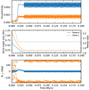 |
Fig. 1 Disc migration and capture in the 2:1 resonance of two planets similar to K2-24b and c. From top to bottom: eccentricity, semi-major axis, and resonant angles θ1 (blue) and θ2 (orange), as defined by Eq. (7). Middle panel: black curve is the period ratio, whose axis is labelled on the right-hand side of the plot. |
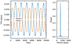 |
Fig. 2 Left: TTV signal for the system obtained at the end of Fig. 1. Right: power spectrum of the signal, showing the peak at ~1580 days. |
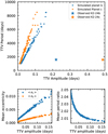 |
Fig. 3 Outcome of all simulations presented in Sect. 3.3. Top panel: TTV amplitude versus TTV period for all the simulated systems. The stars show the observed TTV amplitudes and periods for K2-24 (Petigura et al. 2018). Bottom panels: mean eccentricities (left) and period ratios (right) versus TTV amplitudes of the inner planet for the simulated systems. |
4 Disc-induced precession and eccentricity excitation
It is clear from the previous section that, although it is possible to generate K2-24’s current periods during disc migration, a subsequent mechanism is necessary to excite its eccentricities to a level that can explain the observed TTVs. In this section, we present one such possible scenario.
4.1 Disc-induced precession
In this section, we consider that an inner cavity has been cleared in the disc. In this cavity orbit K2-24b and c, and also K2-24d, the third planet whose possible detection is mentioned by Petigura et al. (2018, see Sect. 2.1). At this point, since all the planets are in the cavity, we assume that they no longer migrate. However, the disc still exerts a gravitational torque on the planets.
Following Teyssandier & Lai (2019), the disc causes interior planets to precess at the rate of
 (22)
(22)
where ap and Ωp are the semi-major axis and Keplerian frequency of the planet. In addition, rin is the inner radius of the disc, and  is the local mass of the disc at the inner radius. Finally,
  is a dimensionless integral whose expression can be found in Teyssandier & Lai (2019).
We assume that the cavity in the disc is such that rin ≳ ad, the semi-major axis of planet d. Hence, in our case, the disc-induced precession is mostly affects planet d. Assuming that the disc slowly dissipates over time, for example due to photoevaporation, the precession rate of planet d slowly changes over time. As shown by Lithwick & Wu (2011), an outer massive planet with a varying precession rate can cause the its interior planets to cross a secular resonance, which would excite their eccentricities.
In order to simulate the effect of the disc dispersal, we assume that  starts from an initial value
  and decays with time as
 (23)
(23)
where tdisp is the dispersal timescale. This simple law is intended to represent whatever process is dispersing the gaseous disc in the later phase of its life, for example photoevaporation or magnetic winds. The disc-induced precession described by Eq. (22) can be readily implemented in REBOUNDx (Tamayo et al. 2020).
4.2 Results
We ran 600 N-body simulations including three planets, the precession term given by Eq. (22), and relativistic corrections. The initial conditions for K2-24b and c are the final parameters of Fig. 1. The mass and semi-major axis of K2-24d are drawn uniformly from the range of possible values quoted by Petigura et al. (2018), that is, [40 M⊕–68 M⊕] and [1.1 au–1.21 au], respectively. Its eccentricity is drawn from a uniform distribution between 0 and 0.3. Its mean longitude and argument of pericentre are drawn from a uniform distribution between 0 and 2π. The three planets and the disc are assumed to be coplanar. The inner radius of the disc is drawn from a uniform distribution between 1.2 and 2 au, while its mass varies uniformly from 5 to 25 MJ. The disc’s surface density is a power law with the index s = 1. The dispersal timescale of the disc varies uniformly between 105 and 3 × 10⁵ yr. With this particular set of parameters, we found that eccentricity excitation of the inner pair was a common outcome of our simulations, with 50% of the simulations resulting in eb > 0.05, and 5% resulting in eb > 0.1.
In Fig. 4, we show an example of evolution of K2-24b and c, as an evaporating disc causes K2-24d to precess at a time-varying rate. The outer planet has the following properties: m3 = 61.2 M⊕ a3 = 1.12 au and e3 = 0.25. The disc extends from rin = 1.8 au to rout = 30 au, and initially contains a mass of 20 MJ. This mass decays exponentially on a timescale of tdisp = 2 × 10⁵ yr. As the disc mass decays in time, it alters the precession of the outer planet, which in turn secularly excites the eccentricity of the inner pair, all while maintaining their semi-major-axis (and therefore period-ratio) constant. The final eccentricities of K2-24b and c are 0.12 and 0.17. Their resonant angles do not librate any more, and the pair is locked in a mutual apsidal precession around 0. The orbit of K2-24d (not shown here) remains largely unaffected. In that sense, K2-24d merely acts as a messenger to propagate a time-varying, secular forcing from the disc onto the interior planets.
In Fig. 5, we show the evolution of Zfree (see Eq. (5)) for the simulation presented in Fig. 4, in the Re (Zfree)–Im(Zfree) plane. At the beginning of the simulation, the free eccentricity of the pair is small since it has been damped during disc migration, and it is therefore concentrated around (0, 0). As the eccentricity is excited, the trajectory expends, until it settles and encompasses the current value of K2-24, which is indicated byan orange star in this plot.
We can now compute the TTVs of the system at the end of the simulation shown in Fig. 4. We show the TTVs in Fig. 6 (with corresponding orbital evolution in Fig. 7). As expected, the signal maintains the same period as before, since the orbital periods have not changed. However, the amplitude of the signal is now much stronger than it was at the end of the disc migration phase (see Fig. 2). In this particular example, the amplitudes are 0.26 and 0.48 days for planets b and c, respectively, which is in good agreement with the observed values reported by Petigura et al. (2018). At the end of the disc-induced migration phase presented in Sect. 3, the TTV amplitude of the inner planet was smaller than that of the outer planet, which was at odds with observations. This is no longer the case. Finally, we note that the periodogram associated with the TTV signal of Fig. 6 shows a small secondary peak at a period of 790 days, which is half of the main period. As noted by Hadden & Lithwick (2016), for a pair of planets near the 2:1 MMR, there is a second harmonic signal associated with the 4:2MMR, whose frequency is twice that of the main signal and whose amplitude is smaller by a factor ~ e. This is the secondary peak that we see on the periodogram of Fig. 6.
In Fig. 7, we show the orbital evolution of planets b and c during the TTV simulated in Fig. 6. We do not show the orbital evolution of planet d, since it is barely affected by the inner pair and its orbital elements do not significantly vary over the time of integration. We see that the orbital elements vary on the same period as the TTVs, and that the system is no longer in resonance. Since ϖb ≃ ϖc, the two resonance angles θ1 and θ2 almost perfectly overlap.
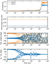 |
Fig. 4 Time evolution of inner pair K2-24b and c, when perturbed by an outer precessing planet and an evaporating disc. From top tobottom: eccentricity, semi-major axis, resonant angles (see Eq. (7)) and difference of argument of pericentres. |
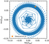 |
Fig. 5 Trajectory of Zfree in real–imaginary plane (see Eq. (5)) for the system shown in Fig. 4. The orange star marks the current observed location of K2-24 in that plane (see Eq. (6)). |
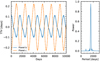 |
Fig. 6 TTV computed at the end of the simulation shown in Fig. 4. The amplitude of each TTV signal, as well as their periods, are the same as those observed in K2-24. |
5 Discussion
5.1 Main assumptions
In order to reproduce the observed properties of K2-24, we built a scenario in two distinct parts. In Sect. 3, we focused on the migration of K2-24b and c in a disc, in order to reproduce their observed period ratio. We did not take into account the presence of the third planet at this stage. We then took the final outcome of one of our simulations, which had the correct period ratio, and used it as the starting point for another set of simulations. This set of simulations, which we presented in Sect. 4, assumed that the disc had partially depleted and formed an inner cavity, and that a third planet also orbited in this cavity. We therefore need to justify two decisions: (i) why did we not take into account planet d in Sect. 3, and (ii) why did we start the simulations of Sect. 4 with a cavity already carved?
Regarding the first point, it is likely that K2-24d formed further out than its current position and migrated in the disc just like K2-24b and c did, but did not have time to reach the inner regions of the disc before it started evaporating. As long as K2-24d did not migrate faster than the inner pair, so as to prevent resonant capture, we assume that the disc would suppress any planet-planet interaction between K2-24d and the inner pair. Therefore their dynamical evolutions would be largely disconnected and the influence of K2-24d can be ignored.
We now discuss the second question. At the end of Sect. 3, we were left with two planets that had stopped migrating at about 0.15 and 0.24 au. This implies that the gaseous disc extended to roughly the same location. However, we started the simulations of Sect. 4 with a disc inner radius at 1.8 au, implying that the disc had cleared an inner cavity. We did not include the intermediate phase where the disc’s inner edge expends from the vicinity of K2-24c to beyond the orbit of K2-24d. As we point out in the next section, it is likely that some instabilities altered the orbit of K2-24d very early on, making the full evolution rather tedious to simulate. Hence, we simplified our assumption to separate the evolution history in two distinct parts.
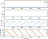 |
Fig. 7 Orbital evolution of planets b and c during TTV simulated in Fig. 6. From top to bottom: semi-major axis, eccentricities, difference of pericenter arguments ϖc − ϖb, and resonantangles θ1 and θ2. |
5.2 Orbital properties of K2-24d
Our mechanism for exciting the eccentricities of planets b and c up to their observed values relies on a secular resonance crossing provoked by the time-varying precession of planet d, induced by an outer disc. As shown by Lithwick & Wu (2011), the strength of this mechanism increases with increasing eccentricity of planet d. In general, we found that eccentricities between 0.2 and 0.3 were adequate. This raises the question of how planet d achieved this eccentricity so early on. Several works have shown that disc-planet interactions can increase the eccentricity of giant, gap-opening planets (see e.g. Papaloizou et al. 2001; Goldreich & Sari 2003; D’Angelo et al. 2006; Rice et al. 2008; Teyssandier & Ogilvie 2016; Ragusa et al. 2018; Muley et al. 2019). However, it is likely that K2-24d is not massive enough for these mechanisms to apply, and it is also not clear whether planet-disc interactions can excite planet eccentricities to such high values. More promisingly, early instabilities of multi-planet systems during disc-planet interactions have been shown to lead to planet–planet scattering (Marzari et al. 2010; Moeckel & Armitage 2012; Lega et al. 2013; Rosotti et al. 2017). This scattering can lead to the ejection of one or more planets, leaving the remaining planet(s) eccentric. If such an event occurred in the outer planetary system of K2-24, it provides a justification for choosing a non-zero eccentricity of K2-24d.
We note that in principle, the two mechanisms discussed above (eccentricity growth due to planet–disc interactions or planet–planet scattering) could also excite the free eccentricity of the inner pair, without having to rely on the existence of a third planet at all. However, there is no evidence that planet–disc interaction can increase the eccentricity of planets in the mass range of K2-24b and c. On the other hand, scattering events result from a kick in orbital energy, and therefore would not preserve the semi-major of the inner pair.
5.3 Disc properties
In Sect. 3, we assumed that the two planets undergo smooth migration in a non-turbulent disc. However, Petigura et al. (2018) argued that the eccentricity of K2-24b and c could be the result of stochastic migration in a turbulent disc (Laughlin et al. 2004; Ogihara et al. 2007; Adams et al. 2008). We implemented the stochastic forces suggested by Laughlin et al. (2004); Ogihara et al. (2007) into our N-body code to test whether stochastic migration could reproduce both the eccentricities and period ratio of K2-24b and c. We found that the turbulent forces had little effect on the outcome once the two planets are captured in a MMR, and therefore we discarded that scenario and did not include turbulent forces in subsequent simulations.
When simulating the migration of the two planets in the disc, we implemented damping formulas from Kanagawa et al. (2018) and Kanagawa & Szuszkiewicz (2020). Although these formulas were used by Kanagawa & Szuszkiewicz (2020) for the migration of two planets, it is worth pointing out that they were derived from hydrodynamical simulations consisting of one planet in a disc. The presence of a second planet would change the disc structure, and the creation of a common gap could slow down the migration rate. In addition, the disc torque may be modified by overlapping spiral density waves, as noted by Brož et al. (2018). The effect of the disc’s self gravity can also modify the migration rate and the occurence of resonant capture (Ataiee & Kley 2020).
5.4 Long-term stability
Finally, we needed to verify that the system obtained in Fig. 4, with its three eccentric planets, is stable over long timescales. We carried an N-body simulation over 100 Myr and observed no destabilisation of the system. Since this does not guarantee the stability of the system over the ageof the system (the star is several Gyr old; see Petigura et al. 2016), we also computed Mean Exponential Growth factor of Nearby Orbits stability maps (MEGNO, which are readily implemented in REBOUND, see also Cincotta & Simó 2000), where we varied the semi-major axis, eccentricity, and mass of K2-24d on a grid of values. The grid extended from ad = 1.1 to ad = 1.21 au, ed = 0.21 to ed = 0.27, and md = 40 M⊕ to md = 68 M⊕. The resolution of the grid was 20 × 20 × 5. These simulations all yielded MEGNO values close to 2, and therefore did not indicate any evidence of chaos in the system.
6 Conclusion
In this paper, we studied the impact of disc-induced migration on the subsequent TTV signal produced by two planets near the 2:1 MMR. We focused on the K2-24 system, and show that disc-induced migration can reproduce the correct ratio of orbital period of the two innermost planets. However, systems formed with the correct period ratio exhibit a TTV signal that is 20 times smaller than the observed TTVs. Hence, in the particular case of K2-24, we suggest that disc-driven migration alone cannot account for the observed properties of the system. We propose that an additional mechanism came into play in the late phase of planet–disc interactions. We found one such possible mechanism, involving the crossing of a secular resonance induced by a third outer planet, whose precession rate is varying due to the evaporating gaseous disc. In this scenario, the planets remain in their observed period ratios, and reach eccentricities that are compatible with observations. The period and amplitude of our simulated TTVs match the observed one.
More generally, we conducted the first study of the impact of disc migration on the amplitude and period of TTV signals. Figure 3 is promising, because it shows that if resonant pairs were formed during disc migration and remained unaltered after that, their TTV signal should lie on a linear track in the amplitude–period diagram. Although this track will be different for each system, direct N-body simulations with migration forces can show whether or not an observed system lies on this track, and shed new light on its formation history.
Acknowledgements
The work of J.T. is supported by a Fonds de la Recherche Scientifique – FNRS Postdoctoral Research Fellowship. Computational resources have been provided by the PTCI (Consortium des Équipements de Calcul Intensif CECI), funded by the FNRS-FRFC, the Walloon Region, and the University of Namur (Conventions No. 2.5020.11, GEQ U.G006.15, 1610468 and RW/GEQ2016). The research done in this project made use of the SciPy stack (Jones et al. 2001), including NumPy (Oliphant 2006) and Matplotlib (Hunter 2007), as well as Astropy (http://www.astropy.org), a community-developed core Python package for Astronomy (Astropy Collaboration 2013, 2018). Simulations in this paper made use of the REBOUND code which is freely available at http://github.com/hannorein/rebound.
References
- Adams, F. C., Laughlin, G., & Bloch, A. M. 2008, ApJ, 683, 1117 [NASA ADS] [CrossRef] [Google Scholar]
- Agol, E., & Fabrycky, D. C. 2018, Handbook of Exoplanets (Cham: Springer), 7 [Google Scholar]
- Agol, E., Steffen, J., Sari, R., & Clarkson, W. 2005, MNRAS, 359, 567 [NASA ADS] [CrossRef] [Google Scholar]
- Astropy Collaboration (Robitaille, T. P., et al.) 2013, A&A, 558, A33 [NASA ADS] [CrossRef] [EDP Sciences] [Google Scholar]
- Astropy Collaboration (Price-Whelan, A. M., et al.) 2018, AJ, 156, 123 [Google Scholar]
- Ataiee, S., & Kley, W. 2020, A&A, 635, A204 [CrossRef] [EDP Sciences] [Google Scholar]
- Batygin, K., & Morbidelli, A. 2013, AJ, 145, 1 [NASA ADS] [CrossRef] [Google Scholar]
- Brož, M., Chrenko, O., Nesvorný, D., & Lambrechts, M. 2018, A&A, 620, A157 [NASA ADS] [CrossRef] [EDP Sciences] [Google Scholar]
- Chatterjee, S.,& Ford, E. B. 2015, ApJ, 803, 33 [NASA ADS] [CrossRef] [Google Scholar]
- Cincotta, P. M., & Simó, C. 2000, A&AS, 147, 205 [NASA ADS] [CrossRef] [EDP Sciences] [Google Scholar]
- Cochran, W. D., Fabrycky, D. C., Torres, G., et al. 2011, ApJS, 197, 7 [NASA ADS] [CrossRef] [Google Scholar]
- Cresswell, P., & Nelson, R. P. 2006, A&A, 450, 833 [NASA ADS] [CrossRef] [EDP Sciences] [Google Scholar]
- Crossfield, I. J. M., Ciardi, D. R., Petigura, E. A., et al. 2016, ApJS, 226, 7 [NASA ADS] [CrossRef] [Google Scholar]
- Dai, F., Winn,J. N., Albrecht, S., et al. 2016, ApJ, 823, 115 [NASA ADS] [CrossRef] [Google Scholar]
- D’Angelo, G., Lubow, S. H., & Bate, M. R. 2006, ApJ, 652, 1698 [NASA ADS] [CrossRef] [Google Scholar]
- Deck, K. M., & Agol, E. 2016, ApJ, 821, 96 [CrossRef] [Google Scholar]
- Delisle, J. B., & Laskar, J. 2014, A&A, 570, L7 [NASA ADS] [CrossRef] [EDP Sciences] [Google Scholar]
- Duffell, P. C., & MacFadyen, A. I. 2013, ApJ, 769, 41 [NASA ADS] [CrossRef] [Google Scholar]
- Fabrycky, D. C., Lissauer, J. J., Ragozzine, D., et al. 2014, ApJ, 790, 146 [Google Scholar]
- Ford, E. B., Fabrycky, D. C., Steffen, J. H., et al. 2012, ApJ, 750, 113 [NASA ADS] [CrossRef] [Google Scholar]
- Fung, J., Shi, J.-M., & Chiang, E. 2014, ApJ, 782, 88 [NASA ADS] [CrossRef] [Google Scholar]
- Goldreich, P., & Sari, R. 2003, ApJ, 585, 1024 [Google Scholar]
- Hadden, S., & Lithwick, Y. 2016, ApJ, 828, 44 [CrossRef] [Google Scholar]
- Hadden, S., & Lithwick, Y. 2017, AJ, 154, 5 [Google Scholar]
- Holman, M. J., & Murray, N. W. 2005, Science, 307, 1288 [NASA ADS] [CrossRef] [PubMed] [Google Scholar]
- Hunter, J. D. 2007, Comput. Sci. Eng., 9, 90 [NASA ADS] [CrossRef] [Google Scholar]
- Jones, E., Oliphant, T., Peterson, P., et al. 2001, SciPy: Open source scientific tools for Python [Google Scholar]
- Kanagawa, K. D., & Szuszkiewicz, E. 2020, ApJ, 894, 59 [CrossRef] [Google Scholar]
- Kanagawa, K. D., Muto, T., Tanaka, H., et al. 2015, ApJ, 806, L15 [NASA ADS] [CrossRef] [Google Scholar]
- Kanagawa, K. D., Tanaka, H., & Szuszkiewicz, E. 2018, ApJ, 861, 140 [NASA ADS] [CrossRef] [Google Scholar]
- Laughlin, G., Steinacker, A., & Adams, F. C. 2004, ApJ, 608, 489 [NASA ADS] [CrossRef] [Google Scholar]
- Lee, M. H. 2004, ApJ, 611, 517 [NASA ADS] [CrossRef] [Google Scholar]
- Lee, M. H., & Peale, S. J. 2002, ApJ, 567, 596 [NASA ADS] [CrossRef] [Google Scholar]
- Lega, E., Morbidelli, A., & Nesvorný, D. 2013, MNRAS, 431, 3494 [NASA ADS] [CrossRef] [Google Scholar]
- Lithwick, Y., & Wu, Y. 2011, ApJ, 739, 31 [NASA ADS] [CrossRef] [Google Scholar]
- Lithwick, Y., & Wu, Y. 2012, ApJ, 756, L11 [NASA ADS] [CrossRef] [Google Scholar]
- Lithwick, Y., Xie, J., & Wu, Y. 2012, ApJ, 761, 122 [NASA ADS] [CrossRef] [Google Scholar]
- Marzari, F., Baruteau, C., & Scholl, H. 2010, A&A, 514, L4 [NASA ADS] [CrossRef] [EDP Sciences] [Google Scholar]
- Masset, F. S., D’Angelo, G., & Kley, W. 2006, ApJ, 652, 730 [NASA ADS] [CrossRef] [Google Scholar]
- Mayo, A. W., Vanderburg, A., Latham, D. W., et al. 2018, AJ, 155, 136 [NASA ADS] [CrossRef] [Google Scholar]
- Miralda-Escudé, J. 2002, ApJ, 564, 1019 [NASA ADS] [CrossRef] [Google Scholar]
- Miranda, R., & Lai, D. 2018, MNRAS, 473, 5267 [NASA ADS] [CrossRef] [Google Scholar]
- Moeckel, N., & Armitage, P. J. 2012, MNRAS, 419, 366 [NASA ADS] [CrossRef] [Google Scholar]
- Muley, D., Fung, J., & van der Marel, N. 2019, ApJ, 879, L2 [CrossRef] [Google Scholar]
- Murray, C. D., & Dermott, S. F. 1999, Solar system dynamics (Cambridge: Cambridge University Press) [Google Scholar]
- Nesvorný, D., & Morbidelli, A. 2008, ApJ, 688, 636 [NASA ADS] [CrossRef] [Google Scholar]
- Novak, G. S., Lai, D., & Lin, D. N. C. 2003, ASP Conf. Ser., 294, 177 [Google Scholar]
- Ogihara, M., Ida, S., & Morbidelli, A. 2007, Icarus, 188, 522 [NASA ADS] [CrossRef] [Google Scholar]
- Oliphant, T. 2006, NumPy: A guide to NumPy (USA: Trelgol Publishing) [Google Scholar]
- Papaloizou, J. C. B., & Larwood, J. D. 2000, MNRAS, 315, 823 [NASA ADS] [CrossRef] [Google Scholar]
- Papaloizou, J. C. B., & Terquem, C. 2010, MNRAS, 405, 573 [NASA ADS] [Google Scholar]
- Papaloizou, J. C. B., Nelson, R. P., & Masset, F. 2001, A&A, 366, 263 [NASA ADS] [CrossRef] [EDP Sciences] [Google Scholar]
- Petigura, E. A., Howard, A. W., Lopez, E. D., et al. 2016, ApJ, 818, 36 [Google Scholar]
- Petigura, E. A., Benneke, B., Batygin, K., et al. 2018, AJ, 156, 89 [Google Scholar]
- Petrovich, C., Malhotra, R., & Tremaine, S. 2013, ApJ, 770, 24 [NASA ADS] [CrossRef] [Google Scholar]
- Ragusa, E., Rosotti, G., Teyssandier, J., et al. 2018, MNRAS, 474, 4460 [NASA ADS] [CrossRef] [Google Scholar]
- Ramos, X. S., Charalambous, C., Benítez-Llambay, P., & Beaugé, C. 2017, A&A, 602, A101 [CrossRef] [EDP Sciences] [Google Scholar]
- Rein, H., & Liu, S. F. 2012, A&A, 537, A128 [NASA ADS] [CrossRef] [EDP Sciences] [Google Scholar]
- Rice, W. K. M., Armitage, P. J., & Hogg, D. F. 2008, MNRAS, 384, 1242 [NASA ADS] [CrossRef] [Google Scholar]
- Rosotti, G. P., Booth, R. A., Clarke, C. J., et al. 2017, MNRAS, 464, L114 [NASA ADS] [CrossRef] [Google Scholar]
- Schneider, J. 2004, ESA SP, 538, 407 [Google Scholar]
- Sinukoff, E., Howard, A. W., Petigura, E. A., et al. 2016, ApJ, 827, 78 [NASA ADS] [CrossRef] [Google Scholar]
- Snellgrove, M. D., Papaloizou, J. C. B., & Nelson, R. P. 2001, A&A, 374, 1092 [NASA ADS] [CrossRef] [EDP Sciences] [Google Scholar]
- Steffen, J. 2006, PhD thesis, University of Washington, Washington [Google Scholar]
- Steffen, J. H., Fabrycky, D. C., Ford, E. B., et al. 2012, MNRAS, 421, 2342 [NASA ADS] [CrossRef] [Google Scholar]
- Tamayo, D., Rein, H., Shi, P., & Hernand ez, D. M. 2020, MNRAS, 491, 2885 [CrossRef] [Google Scholar]
- Tanaka, H., & Ward, W. R. 2004, ApJ, 602, 388 [NASA ADS] [CrossRef] [Google Scholar]
- Tanaka, H., Takeuchi, T., & Ward, W. R. 2002, ApJ, 565, 1257 [NASA ADS] [CrossRef] [Google Scholar]
- Terquem, C., & Papaloizou, J. C. B. 2019, MNRAS, 482, 530 [CrossRef] [Google Scholar]
- Teyssandier, J., & Lai, D. 2019, MNRAS, 490, 4353 [CrossRef] [Google Scholar]
- Teyssandier, J., & Ogilvie, G. I. 2016, MNRAS, 458, 3221 [NASA ADS] [CrossRef] [Google Scholar]
- Teyssandier, J., & Terquem, C. 2014, MNRAS, 443, 568 [NASA ADS] [CrossRef] [Google Scholar]
- Tsang, D. 2011, ApJ, 741, 109 [CrossRef] [Google Scholar]
- Wu, Y., & Lithwick, Y. 2013, ApJ, 772, 74 [NASA ADS] [CrossRef] [Google Scholar]
In this paper, we define the “exact commensurability” as the ratio of two integers. Hence, the exact commensurability associated with the 2:1 MMR is 2. Broadly speaking, planet pairs whose orbital period ratios fall near the exact commensurability are refered to as being “near” the resonance, regardless of whether or not they are resonant in the dynamical sense.
All Tables
All Figures
|
Fig. 1 Disc migration and capture in the 2:1 resonance of two planets similar to K2-24b and c. From top to bottom: eccentricity, semi-major axis, and resonant angles θ1 (blue) and θ2 (orange), as defined by Eq. (7). Middle panel: black curve is the period ratio, whose axis is labelled on the right-hand side of the plot. |
| In the text | |
|
Fig. 2 Left: TTV signal for the system obtained at the end of Fig. 1. Right: power spectrum of the signal, showing the peak at ~1580 days. |
| In the text | |
|
Fig. 3 Outcome of all simulations presented in Sect. 3.3. Top panel: TTV amplitude versus TTV period for all the simulated systems. The stars show the observed TTV amplitudes and periods for K2-24 (Petigura et al. 2018). Bottom panels: mean eccentricities (left) and period ratios (right) versus TTV amplitudes of the inner planet for the simulated systems. |
| In the text | |
|
Fig. 4 Time evolution of inner pair K2-24b and c, when perturbed by an outer precessing planet and an evaporating disc. From top tobottom: eccentricity, semi-major axis, resonant angles (see Eq. (7)) and difference of argument of pericentres. |
| In the text | |
|
Fig. 5 Trajectory of Zfree in real–imaginary plane (see Eq. (5)) for the system shown in Fig. 4. The orange star marks the current observed location of K2-24 in that plane (see Eq. (6)). |
| In the text | |
|
Fig. 6 TTV computed at the end of the simulation shown in Fig. 4. The amplitude of each TTV signal, as well as their periods, are the same as those observed in K2-24. |
| In the text | |
|
Fig. 7 Orbital evolution of planets b and c during TTV simulated in Fig. 6. From top to bottom: semi-major axis, eccentricities, difference of pericenter arguments ϖc − ϖb, and resonantangles θ1 and θ2. |
| In the text | |
Current usage metrics show cumulative count of Article Views (full-text article views including HTML views, PDF and ePub downloads, according to the available data) and Abstracts Views on Vision4Press platform.
Data correspond to usage on the plateform after 2015. The current usage metrics is available 48-96 hours after online publication and is updated daily on week days.
Initial download of the metrics may take a while.