| Issue |
A&A
Volume 642, October 2020
|
|
|---|---|---|
| Article Number | A159 | |
| Number of page(s) | 7 | |
| Section | The Sun and the Heliosphere | |
| DOI | https://doi.org/10.1051/0004-6361/202038557 | |
| Published online | 15 October 2020 | |
Simultaneous transverse oscillations of a coronal loop and a filament excited by a circular-ribbon flare⋆
1
Key Laboratory of Dark Matter and Space Astronomy, Purple Mountain Observatory, CAS, Nanjing 210023, PR China
e-mail: zhangqm@pmo.ac.cn
2
School of Astronomy and Space Science, Nanjing University, Nanjing 210023, PR China
3
State Key Laboratory of Space Weather, Chinese Academy of Sciences, Beijing 100190, PR China
4
State Key Laboratory of Lunar and Planetary Sciences, Macau University of Science and Technology, Macau, PR China
Received:
2
June
2020
Accepted:
4
August
2020
Aims. The aim of this study is to investigate the excitation of kink oscillations in coronal loops and filaments, by analyzing a C3.4 circular-ribbon flare associated with a blowout jet in active region 12434 on 2015 October 16.
Methods. The flare was observed in ultraviolet and extreme-ultraviolet wavelengths by the Atmospheric Imaging Assembly on board the Solar Dynamics Observatory (SDO) spacecraft. The line-of-sight (LOS) magnetograms of the photosphere were observed by the Helioseismic and Magnetic Imager on board SDO. Soft X-ray fluxes of the flares in 0.5−4 and 1−8 Å were recorded by the GOES spacecraft.
Results. The flare excited small-amplitude kink oscillation of a remote coronal loop. The oscillation lasted for ≥4 cycles without significant damping. The amplitude and period are 0.3 ± 0.1 Mm and 207 ± 12 s. Interestingly, the flare also excited transverse oscillation of a remote filament. The oscillation lasted for ∼3.5 cycles with decaying amplitudes. The initial amplitude is 1.7−2.2 Mm. The period and damping time are 437−475 s and 1142−1600 s. The starting times of simultaneous oscillations of coronal loop and filament were concurrent with the hard X-ray peak time. Though small in size and short in lifetime, the flare set off a chain reaction. It generated a bright secondary flare ribbon (SFR) in the chromosphere, remote brightening (RB) that was cospatial with the filament, and intermittent, jet-like flow propagating in the northeast direction.
Conclusions. The loop oscillation is most probably excited by the flare-induced blast wave at a speed of ≥1300 km s−1. The excitation of the filament oscillation is more complicated. The blast wave triggers secondary magnetic reconnection far from the main flare, which not only heats the local plasma to higher temperatures (SFR and RB), but produces jet-like flow (i.e., reconnection outflow) as well. The filament is disturbed by the secondary magnetic reconnection and experiences transverse oscillation. These findings provide new insight into the excitation of transverse oscillations of coronal loops and filaments.
Key words: Sun: flares / Sun: filaments / prominences / Sun: oscillations
Movies associated to Figs. 2 and 6 are available at https://www.aanda.org
© ESO 2020
1. Introduction
Waves and oscillations are prevalent in the solar atmosphere (see Oliver & Ballester 2002; Nakariakov & Verwichte 2005; Arregui et al. 2012; De Moortel & Nakariakov 2012, and references therein). After being disturbed by an external driver, a static coronal loop may deviate from its equilibrium position and experience oscillations (Edwin & Roberts 1983). Transverse coronal loop oscillations are most frequently excited by adjacent solar flares (Aschwanden et al. 1999; Nakariakov et al. 1999; Wang & Solanki 2004; Zimovets & Nakariakov 2015; Li et al. 2017, 2020) and occasionally by shock waves (Hudson & Warmuth 2004) or coronal extreme-ultraviolet (EUV) waves (Kumar et al. 2013). The initial amplitudes of loop displacement range from a few to 30 Mm and most of them are less than 10 Mm (Nechaeva et al. 2019). Two quantities, namely the loop length and density contrast, play a relevant role in determining the amplitude of oscillation (Terradas et al. 2007). Goddard et al. (2016a) analyzed 58 kink oscillation events observed by the Atmospheric Imaging Assembly (AIA; Lemen et al. 2012) on board the Solar Dynamics Observatory (SDO) during its first four years of operation. It is found that the period is proportional to the loop length (Goddard & Nakariakov 2016b). The commonly observed transverse oscillations of standing kink mode provide a useful tool to infer the magnetic field strength and Alfvén speed of the coronal loops, which are hard to measure in a direct way (Nakariakov & Ofman 2001; Verwichte et al. 2004; Van Doorsselaere et al. 2008; White & Verwichte 2012; Yuan & Van Doorsselaere 2016; Arregui et al. 2019). Some of the small-amplitude (≲0.5 Mm) oscillations hardly attenuate with time, which are called decayless oscillations (Anfinogentov et al. 2013, 2015; Li et al. 2018a). Nisticò et al. (2013) reported small-amplitude, decayless loop oscillations before a flare and high-amplitude, decaying oscillations after the flare.
Circular-ribbon flares (CRFs) are a special type of flares, whose outer ribbons surrounding the compact inner ribbons show a circular or elliptical shape (Masson et al. 2009; Zhang et al. 2016). Like typical two-ribbon flares, CRFs are also capable of triggering transverse loop oscillations (Li et al. 2018b). Zhang et al. (2020a) investigated the transverse oscillations of an EUV loop excited by two homologous CRFs on 2014 March 5. The oscillations are divided into two stages in their development: the first-stage oscillation triggered by the C2.8 flare is decayless with lower amplitudes (310−510 km), and the second-stage oscillation triggered by the M1.0 flare is decaying with larger amplitudes (1250−1280 km).
Large-amplitude prominence or filament oscillations are divided into two categories according to their directions: transverse and longitudinal oscillations (Hyder 1966; Ramsey & Smith 1966; Kleczek & Kuperus 1969; Tripathi et al. 2009; Luna et al. 2018). Longitudinal oscillations can be triggered by microflares (Jing et al. 2003; Vršnak et al. 2007; Zhang et al. 2012, 2017a), flares (Li & Zhang 2012; Zhang et al. 2020b), coronal jets (Luna et al. 2014), shock waves (Shen et al. 2014), and failed filament eruptions (Mazumder et al. 2020). Transverse prominence oscillations are often excited by Moreton waves and/or EUV waves from a remote site of eruption at speeds of ∼1000 km s−1 (e.g., Eto et al. 2002; Gilbert et al. 2008; Hershaw et al. 2011; Asai et al. 2012; Dai et al. 2012; Gosain & Foullon 2012; Liu et al. 2012; Shen et al. 2017; Zhang & Ji 2018). Sometimes, they are triggered by magnetic reconnection as a result of magnetic flux emergence (Isobe & Tripathi 2006; Chen et al. 2008). When an EUV jet from a remote AR arrives and collides with a filament, transverse oscillation of the filament may be generated (Zhang et al. 2017b). Sophisticated numerical simulations have shed light on the triggering mechanism, restoring force, and damping mechanism of filament oscillations (e.g., Luna & Karpen 2012; Zhang et al. 2013; Zhou et al. 2018; Adrover-González & Terradas 2020; Fan 2020; Jelínek et al. 2020; Liakh et al. 2020). Several damping mechanisms have been proposed to interpret the observed attenuation of filament oscillations, such as thermal effects, resonant absorption in nonuniform media, and partial ionization effects (see Arregui & Ballester 2011, and references therein).
So far, the excitation of kink oscillations in coronal loops and filaments is still controversial. The motivation of this study is to investigate a C3.4 CRF in NOAA active region (AR) 12434, which excited transverse oscillations of a remote coronal loop and a remote filament on 2015 October 16. This paper is organized as follows. Observations and results are presented in Sect. 2. The possible origin of kink oscillations is discussed in Sect. 3. Finally, a brief summary is given in Sect. 4.
2. Observations and results
2.1. Instruments and data analysis
The C3.4 flare was observed by SDO/AIA. The AIA takes full-disk images in two ultraviolet (UV; 1600 and 1700 Å) and seven EUV (94, 131, 171, 193, 211, 304, and 335 Å) wavelengths. The line-of-sight (LOS) magnetograms of the photosphere were observed by the Helioseismic and Magnetic Imager (HMI; Scherrer et al. 2012) on board SDO. The level_1 data of AIA and HMI were calibrated using the standard solar software (SSW) program aia_prep.pro and hmi_prep.pro, respectively. Soft X-ray (SXR) light curves of the flare in 0.5−4 and 1−8 Å were recorded by the GOES spacecraft. The observational parameters during 08:50−09:30 UT are listed in Table 1.
Description of the observational parameters.
2.2. Flare and blowout jet
The top panel of Fig. 1 shows SXR light curves of the flare. The SXR emissions started to rise at ∼08:57 UT and reached peak values at ∼09:03 UT before declining gradually until ∼09:12 UT. Therefore, the lifetime of the flare is ∼15 min, which is equal to that of the homologous C3.1 flare starting at ∼10:15 UT (Zhang et al. 2016). Figure 1b shows the time derivative of the 1−8 Å flux, which serves as a hard X-ray (HXR) proxy according to the Neupert effect. The HXR emission peaks at ∼09:01:00 UT. The light curve of the flare in AIA 1600 Å, which is calculated by integrating the intensities of the flare region in Fig. 2f, is plotted in Fig. 1c. The UV emission reaches its maximum ∼40 s before the HXR peak. Combining the UV and HXR light curves of the flare, it is concluded that the most impulsive release of energy occurred during 09:00−09:01 UT.
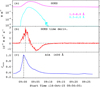 |
Fig. 1. Panel a: SXR light curves of the C3.4 flare in 0.5−4 Å (cyan line) and 1−8 Å (magenta line). Panel b: time derivative of the 1−8 Å flux. Panel c: light curve of the flare in AIA 1600 Å. |
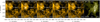 |
Fig. 2. Panels a–e: snapshots of the AIA 171 Å images. The arrows point to the CRF, bright loop, and dark filament. The white box in panel b signifies the flare region. Panel f: close-up of the flare region in AIA 1600 Å. The whole evolution is shown in a movie available online. |
In Fig. 2, the EUV images in 171 Å demonstrate the whole evolution of the event. The EUV intensities of the flare started to increase at ∼08:58 UT and reached peak values at ∼09:00 UT (see panels a and b). The flare was accompanied by a curved blowout jet propagating in the southeast direction, which was observed in UV and EUV wavelengths (see panels c–f). The jet did not appear in the C2 white light (WL) coronagraph of the Large Angle Spectroscopic Coronagraph (LASCO; Brueckner et al. 1995) on board SOHO1, indicating that it did not evolve into a narrow coronal mass ejection (CME). Hence, the jet-related flare was a confined flare rather than an eruptive one.
2.3. Coronal loop oscillation
The flare excited transverse oscillation of a coronal loop, which is ∼230″ away from the flare site (see Fig. 2 and online movie). It should be emphasized that only the western part of the oscillating loop close to the footpoint is clearly observed in EUV wavelengths. To better illustrate the displacements of the loop, the running difference technique is applied to the original EUV images. Running-difference images in 171 Å during 09:04−09:09 UT are displayed in the top panels of Fig. 3. The blue (red) color represents intensity enhancement (weakening), respectively. It is clear that the loop segment oscillated back and forth in a coherent way. Since the remaining segment of the loop is not visible, whether the kink oscillation is fundamental or harmonic is unknown.
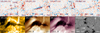 |
Fig. 3. Panels a–d: running-difference images in 171 Å, where blue (red) color represents intensity enhancement (weakening). The slice (S1) is used to investigate the loop oscillation. Panels e–g: close-ups of the filament in 171, 193, and 211 Å. The slice (S2) is used to investigate the filament oscillation. Panel h: HMI LOS magnetogram associated with the filament. The field of view of each panel is 90″ × 60″. |
The loop oscillation is most definitely recognized in 171 Å. To quantify the characteristics of the oscillation, an artificial slice (S1) with a length of 12″ across the loop is selected (see Fig. 3a). Time−distance diagram of S1 in 171 Å is shown in Fig. 4a. The magenta plus symbols denote the central positions of the loop. The small-amplitude oscillation commenced at ∼09:01 UT and lasted for several cycles without significant damping. The loop also experienced slight linear drifting motion at a speed of ∼0.6 km s−1, which is listed in the second column of Table 2.
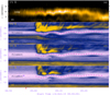 |
Fig. 4. Panel a: time−distance diagram of S1 in 171 Å showing the transverse oscillation of the coronal loop. The magenta plus symbols denote the central positions of the loop. On the y-axis, s = 0 and s = 12″ denote the south and north endpoints of S1, respectively. Panels b–d: time−distance diagrams of S2 in different wavelengths showing the transverse oscillation of the filament. The magenta plus symbols denote the central positions of the filament. On the y-axis, s = 0 and s = 48″ denote the south and north endpoints of S2, respectively. The red arrow on the x-axis signifies the start time of C3.4 flare in SXR. |
Parameters of transverse loop oscillation (LO) and filament oscillation (FO) observed by AIA in different wavelengths.
The detrended central position of the loop is drawn with cyan circles in Fig. 5a. Likewise, it is fitted with a decayless sine function using the standard SSW program mpfit.pro (Zhang et al. 2020a):
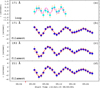 |
Fig. 5. Panel a: detrended central positions of the coronal loop in 171 Å. Kink oscillation of the loop is fitted with a decayless (magenta line) sine function. Panels b–d: detrended central positions of the filament in 171, 193, and 211 Å. Transverse oscillation of the filament is fitted with an exponentially decaying (red lines) sine function. |
where A1 and ϕ1 stand for the initial amplitude of displacement and phase, respectively, and P1 denotes the period. The derived values of A1 = 0.3 ± 0.1 Mm and P1 = 207 ± 12 s are listed in the third and fourth columns of Table 2. In order to estimate the uncertainties of A1 and P1, one hundred Markov chain Monte Carlo (MCMC; Sharma 2017) samplings of y1 are computed. For each MC simulation, y1 is perturbed by a small amount, which is randomly drawn from normal distribution with 1σ being equal to the uncertainty of y1. The curve fitting using mpfit.pro is repeated for each of the 100 MC realizations (Cheng et al. 2012). The uncertainties of A1 and P1 are given at the 95% credible interval (Arregui et al. 2019).
The amplitude of loop oscillation in this study is slightly lower than that of the EUV loop during its decayless oscillation on 2014 March 5 (Zhang et al. 2020a). Terradas et al. (2007) examined the energy that an initial disturbance stores in the eigenmodes of coronal loops. It is found that the trapped energy in coronal loops decreases quickly with the distance of the pertubation, which can explain the small amplitude of the oscillating loop that is ∼230″ away from the flare region.
Terradas et al. (2005) investigated the excitation of trapped and leaky modes in coronal slabs. The leaky modes are characterized by short-period oscillations and fast attenuations. Trapped modes, on the contrary, have much longer periods and marginal attenuations. The observed decayless kink oscillation of the coronal loop in Fig. 4a belongs to the trapped mode. The leaky mode before the trapped mode was absent, owing to the short period and damping time (Terradas et al. 2005).
2.4. Filament oscillation
Interestingly, the flare not only excited kink oscillation of the coronal loop as described above, but also triggered transverse oscillation of the remote filament in the quiet region (see Fig. 2 and online movie). Close-ups of the filament observed at ∼09:01 UT in 171, 193, and 211 Å are depicted in Figs. 3e–g. The filament, consisting of fine dark threads, shows an ℒ-shape. The LOS magnetogram associated with the filament is displayed in Fig. 3h, where negative magnetic polarities dominate. To investigate the filament oscillation, an artificial slice (S2) crossing the filament with a length of 48″ is selected in Fig. 3e. Time−distance diagrams of S2 in different wavelengths are displayed in Figs. 4b–d, where magenta plus symbols represent the central positions of the filament during the oscillation. The oscillation started at ∼09:01 UT and lasted for a few cycles with damping amplitudes. Linear drifting motion of the filament at a speed of ∼1.6 km s−1 is extracted from the diagrams (see the second column of Table 2).
To derive parameters of the kink oscillation, detrended central positions of the filament in different wavelengths are plotted with blue circles in Figs. 5b–d. They are fitted with an exponentially decaying sine function (Zhang et al. 2020a):
where A2 and ϕ2 stand for the initial amplitude of displacement and phase, and P2 and τ2 signify the period and damping time. The fitted values of A2, P2, τ2, and  are listed in the middle four columns of Table 2. The corresponding uncertainties of these parameters are obtained using the same method of MC simulation as described in Sect. 2.3.
3. Discussion
Transverse oscillations are ubiquitous in the solar atmosphere, especially in coronal loops and prominences (Ruderman & Erdélyi 2009). Zimovets & Nakariakov (2015) analyzed 58 kink-oscillation events observed by SDO/AIA. The main conclusion of their work is that in nearly all events the excitation of kink oscillations is caused by the displacement of the loops from their equilibrium state as a result of a nearby lower coronal eruption/ejection and subsequent oscillatory relaxation of the loops. On the contrary, the blast wave plays a minor role in the excitation. In this study, the start time of loop oscillation is concurrent with the HXR peak time of the flare (see Figs. 1 and 5). It is noted that the start times of both decayless and decaying loop oscillations were also coincident with the HXR peaks on 2014 March 5 (Zhang et al. 2020a), suggesting that the excitation of kink oscillations is related to the most impulsive release of magnetic energy rather than the very beginning of energy release. Hence, the real speeds of the driver can potentially reach ∼1000 km s−1, the typical speed of a blast wave (Tothova et al. 2011).
From the online movie of Fig. 2, a plausible signature of blast wave is crudely identified by eye. Figure 6 shows snapshots of the base-ratio images in 211 and 304 Å. The jet-related CRF, though small in size and short in lifetime, sets off a chain reaction. It generates large-scale remote dimming, a bright secondary flare ribbon (SFR) in the chromosphere, remote brightening (RB) that is cospatial with the filament, and jet-like flow propagating in the northeast direction. In Fig. 6d, a long artificial slice (S3), starting from the flare site and passing through the oscillating loop, is selected to investigate the plausible blast wave. Time−distance diagrams of S3 in different EUV wavelengths are plotted in Fig. 7. A sharp linear structure coincident with the UV and HXR peaks during 09:00−09:01 UT is evident in all wavelengths. Using the slopes of the structure, the apparent speeds are calculated to be ∼1340 km s−1, which is of the same order of magnitude as blast waves in the corona (Hudson & Warmuth 2004; Tothova et al. 2011). The kink oscillation of the loop commences after the blast wave arrives. Therefore, the driver of loop oscillation is most probably the flare-induced blast wave.
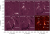 |
Fig. 6. Base-ratio images in 211 Å (panels a–e) and 304 Å (panel f). The white arrows point to the CRF, blowout jet, dark dimming, secondary flare ribbon, remote brightening, and jet-like flow. Panel d: S3 is used to measure the speeds of a plausible blast wave. S4 is used to calculate the speeds of jet-like flow propagating in the northeast direction. The whole evolution is shown in a movie available online. |
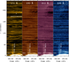 |
Fig. 7. Time−distance diagrams of S3 in different EUV wavelengths. The apparent speeds of the plausible blast wave are labeled. On the y-axis, s = 0 and s = 288″ denote the flare site and southwest endpoint of S3. |
Zhang et al. (2014) investigated the flare ribbons of 19 X-class flares observed by SDO/AIA, finding that 11 of the 16 well-detected events show multiple ribbons. The authors divided the ribbons into two types: normal ribbons that are connected by the post-flare loops (PFLs) and SFRs. The short-period SFRs, usually weaker than the primary ribbons, are not connected by PFLs. It is suggested that the magnetic reconnection associated with the SFRs is probably triggered by the flare-induced blast wave. In this study of the C3.4 flare, it generates a SFR observed in 304 Å (see Fig. 6f). Meanwhile, the RB cospatial with the filament and jet-like flow propagating in the northeast direction are observed by AIA in EUV wavelengths, implying their multithermal nature. In Fig. 6d, a curved slice (S4) is selected to investigate the plasma flow. Time-slice diagrams of S4 in different EUV wavelengths are displayed in Fig. 8. Intermittent plasma flow, originating from the RB and propagating at speeds of ∼140 km s−1, is clearly demonstrated. The starting times of filament oscillation and jet-like flow are consistent with each other.
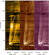 |
Fig. 8. Time-distance diagrams of S4 in 171, 193 and 211 Å. The apparent speed (∼140 km s−1) of the jet-like flow is labeled. On the y-axis, s = 0 and s = 301″ denote the south and north endpoints of S4. |
Inspired by the conjecture of Zhang et al. (2014), it is proposed that the flare-induced blast wave causes secondary magnetic reconnection far from the primary flare, which not only heats the local plasma to higher temperatures (SFR and RB), but produces jet-like flow (i.e., reconnection outflow) as well. Meanwhile, the filament is disturbed by the magnetic reconnection and experiences transverse oscillation. The oscillating threads with the highest amplitude and longest cycles are tightly cospatial with the source of plasma flow (see Fig. 3e). The remaining part of the filament oscillated in the same direction with much faster damping and shorter lifetime (1−2 cycles). Hence, the excitation of filament oscillation in this event is much more complicated than the situation in previously reported events where filament oscillations are directly excited when fast coronal EUV waves or Moreton waves impact the filaments from the side (e.g., Eto et al. 2002; Hershaw et al. 2011; Dai et al. 2012; Gosain & Foullon 2012; Liu et al. 2012; Shen et al. 2017). The plausible blast wave is not a shock wave, since the type II radio burst associated with the shock wave was not observed. It is noted that the scenario of kink oscillations triggered by a blast wave is a conjecture (see Fig. 9), which needs to be validated in the future. The oscillations of coronal loop and filament could not be triggered by the blowout jet because the jet propagated in the southeast direction and covered a limited distance.
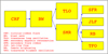 |
Fig. 9. Timeline of the whole event to illustrate a plausible scenario of transverse oscillations in a remote coronal loop and a remote filament excited by the CRF. |
4. Summary
In this work, a C3.4 CRF associated with a blowout jet in AR 12434 on 2015 October 16 is studied. The main results are summarized as follows:
-
The flare excited small-amplitude kink oscillation of a remote coronal loop. The oscillation lasted for ≥4 cycles without significant damping. The amplitude and period are 0.3 ± 0.1 Mm and 207 ± 12 s, respectively. Intriguingly, the flare also excited transverse oscillation of a remote filament. The oscillation lasted for ∼3.5 cycles with decaying amplitudes. The initial amplitude is 1.7−2.2 Mm. The period and damping time are 437−475 s and 1142−1600 s. The starting times of simultaneous oscillations of the coronal loop and filament were concurrent with the HXR peak time.
-
Though small in size and short in lifetime, the flare set off a chain reaction. It generated a bright SFR in the chromosphere, RB that was cospatial with the filament, and intermittent, jet-like flow propagating in the northeast direction. The loop oscillation is most probably excited by the flare-induced blast wave at a speed of ≥1300 km s−1. The excitation of the filament oscillation is more complicated. The blast wave triggers secondary magnetic reconnection far from the primary flare, which not only heats the local plasma to higher temperatures (SFR and RB), but produces intermittent, jet-like flow (i.e., reconnection outflow) as well. The filament is disturbed by the secondary magnetic reconnection and experiences transverse oscillation. The results are important to understand the excitation of transverse oscillations of coronal loops and filaments.
Movies
Movie of Fig. 2 Access here
Movie of Fig. 6 Access here
Acknowledgments
The author is thankful for valuable comments and suggestions from the referee. The author appreciates Prof. Jun Zhang and Prof. Song Feng for inspiring discussion. SDO is a mission of NASA’s Living With a Star Program. AIA and HMI data are courtesy of the NASA/SDO science teams. This work is funded by NSFC grants (No. 11773079, 11790302), the International Cooperation and Interchange Program (11961131002), the Youth Innovation Promotion Association CAS, the Science and Technology Development Fund of Macau (275/2017/A), CAS Key Laboratory of Solar Activity, National Astronomical Observatories (KLSA202006), and the project supported by the Specialized Research Fund for State Key Laboratories.
References
- Adrover-González, A., & Terradas, J. 2020, A&A, 633, A113 [NASA ADS] [CrossRef] [EDP Sciences] [Google Scholar]
- Anfinogentov, S., Nisticò, G., & Nakariakov, V. M. 2013, A&A, 560, A107 [NASA ADS] [CrossRef] [EDP Sciences] [Google Scholar]
- Anfinogentov, S. A., Nakariakov, V. M., & Nisticò, G. 2015, A&A, 583, A136 [NASA ADS] [CrossRef] [EDP Sciences] [Google Scholar]
- Arregui, I., & Ballester, J. L. 2011, Space Sci. Rev., 158, 169 [NASA ADS] [CrossRef] [Google Scholar]
- Arregui, I., Oliver, R., & Ballester, J. L. 2012, Liv. Rev. Sol. Phys., 9, 2 [Google Scholar]
- Arregui, I., Montes-Solís, M., & Asensio Ramos, A. 2019, A&A, 625, A35 [CrossRef] [EDP Sciences] [Google Scholar]
- Asai, A., Ishii, T. T., Isobe, H., et al. 2012, ApJ, 745, L18 [NASA ADS] [CrossRef] [Google Scholar]
- Aschwanden, M. J., Fletcher, L., Schrijver, C. J., et al. 1999, ApJ, 520, 880 [NASA ADS] [CrossRef] [Google Scholar]
- Brueckner, G. E., Howard, R. A., Koomen, M. J., et al. 1995, Sol. Phys., 162, 357 [NASA ADS] [CrossRef] [Google Scholar]
- Chen, P. F., Innes, D. E., & Solanki, S. K. 2008, A&A, 484, 487 [NASA ADS] [CrossRef] [EDP Sciences] [Google Scholar]
- Cheng, X., Zhang, J., Saar, S. H., et al. 2012, ApJ, 761, 62 [NASA ADS] [CrossRef] [Google Scholar]
- Dai, Y., Ding, M. D., Chen, P. F., et al. 2012, ApJ, 759, 55 [NASA ADS] [CrossRef] [Google Scholar]
- De Moortel, I., & Nakariakov, V. M. 2012, Phil. Trans. R. Soc. London Ser. A, 370, 3193 [Google Scholar]
- Edwin, P. M., & Roberts, B. 1983, Sol. Phys., 88, 179 [NASA ADS] [CrossRef] [Google Scholar]
- Eto, S., Isobe, H., Narukage, N., et al. 2002, PASJ, 54, 481 [NASA ADS] [CrossRef] [Google Scholar]
- Fan, Y. 2020, ApJ, 898, 34 [CrossRef] [Google Scholar]
- Gilbert, H. R., Daou, A. G., Young, D., Tripathi, D., & Alexander, D. 2008, ApJ, 685, 629 [NASA ADS] [CrossRef] [Google Scholar]
- Goddard, C. R., Nisticò, G., Nakariakov, V. M., et al. 2016a, A&A, 585, A137 [NASA ADS] [CrossRef] [EDP Sciences] [Google Scholar]
- Goddard, C. R., & Nakariakov, V. M. 2016b, A&A, 590, L5 [NASA ADS] [CrossRef] [EDP Sciences] [Google Scholar]
- Gosain, S., & Foullon, C. 2012, ApJ, 761, 103 [CrossRef] [Google Scholar]
- Hershaw, J., Foullon, C., Nakariakov, V. M., et al. 2011, A&A, 531, A53 [NASA ADS] [CrossRef] [EDP Sciences] [Google Scholar]
- Hudson, H. S., & Warmuth, A. 2004, ApJ, 614, L85 [NASA ADS] [CrossRef] [Google Scholar]
- Hyder, C. L. 1966, Z. Astroph., 63, 78 [Google Scholar]
- Isobe, H., & Tripathi, D. 2006, A&A, 449, L17 [NASA ADS] [CrossRef] [EDP Sciences] [Google Scholar]
- Jelínek, P., Karlický, M., Smirnova, V. V., et al. 2020, A&A, 637, A42 [CrossRef] [EDP Sciences] [Google Scholar]
- Jing, J., Lee, J., Spirock, T. J., et al. 2003, ApJ, 584, L103 [NASA ADS] [CrossRef] [Google Scholar]
- Kleczek, J., & Kuperus, M. 1969, Sol. Phys., 6, 72 [NASA ADS] [CrossRef] [Google Scholar]
- Kumar, P., Cho, K.-S., Chen, P. F., et al. 2013, Sol. Phys., 282, 523 [NASA ADS] [CrossRef] [Google Scholar]
- Lemen, J. R., Title, A. M., Akin, D. J., et al. 2012, Sol. Phys., 275, 17 [Google Scholar]
- Li, T., & Zhang, J. 2012, ApJ, 760, L10 [NASA ADS] [CrossRef] [Google Scholar]
- Li, D., Ning, Z. J., Huang, Y., et al. 2017, ApJ, 849, 113 [NASA ADS] [CrossRef] [Google Scholar]
- Li, D., Yuan, D., Su, Y. N., et al. 2018a, A&A, 617, A86 [NASA ADS] [CrossRef] [EDP Sciences] [Google Scholar]
- Li, T., Yang, S., Zhang, Q., et al. 2018b, ApJ, 859, 122 [NASA ADS] [CrossRef] [Google Scholar]
- Li, D., Li, Y., Lu, L., et al. 2020, ApJ, 893, L17 [Google Scholar]
- Liakh, V., Luna, M., & Khomenko, E. 2020, A&A, 637, A75 [CrossRef] [EDP Sciences] [Google Scholar]
- Liu, W., Ofman, L., Nitta, N. V., et al. 2012, ApJ, 753, 52 [NASA ADS] [CrossRef] [Google Scholar]
- Luna, M., & Karpen, J. 2012, ApJ, 750, L1 [NASA ADS] [CrossRef] [Google Scholar]
- Luna, M., Knizhnik, K., Muglach, K., et al. 2014, ApJ, 785, 79 [NASA ADS] [CrossRef] [Google Scholar]
- Luna, M., Karpen, J., Ballester, J. L., et al. 2018, ApJS, 236, 35 [NASA ADS] [CrossRef] [Google Scholar]
- Masson, S., Pariat, E., Aulanier, G., et al. 2009, ApJ, 700, 559 [NASA ADS] [CrossRef] [Google Scholar]
- Mazumder, R., Pant, V., Luna, M., et al. 2020, A&A, 633, A12 [NASA ADS] [CrossRef] [EDP Sciences] [Google Scholar]
- Nakariakov, V. M., & Ofman, L. 2001, A&A, 372, L53 [NASA ADS] [CrossRef] [EDP Sciences] [Google Scholar]
- Nakariakov, V. M., & Verwichte, E. 2005, Liv. Rev. Sol. Phys., 2, 3 [Google Scholar]
- Nakariakov, V. M., Ofman, L., Deluca, E. E., et al. 1999, Science, 285, 862 [Google Scholar]
- Nechaeva, A., Zimovets, I. V., Nakariakov, V. M., et al. 2019, ApJS, 241, 31 [NASA ADS] [CrossRef] [Google Scholar]
- Nisticò, G., Nakariakov, V. M., & Verwichte, E. 2013, A&A, 552, A57 [NASA ADS] [CrossRef] [EDP Sciences] [Google Scholar]
- Oliver, R., & Ballester, J. L. 2002, Sol. Phys., 206, 45 [NASA ADS] [CrossRef] [Google Scholar]
- Ramsey, H. E., & Smith, S. F. 1966, AJ, 71, 197 [NASA ADS] [CrossRef] [Google Scholar]
- Ruderman, M. S., & Erdélyi, R. 2009, Space Sci. Rev., 149, 199 [NASA ADS] [CrossRef] [Google Scholar]
- Scherrer, P. H., Schou, J., Bush, R. I., et al. 2012, Sol. Phys., 275, 207 [Google Scholar]
- Sharma, S. 2017, ARA&A, 55, 213 [NASA ADS] [CrossRef] [Google Scholar]
- Shen, Y., Liu, Y. D., Chen, P. F., et al. 2014, ApJ, 795, 130 [NASA ADS] [CrossRef] [Google Scholar]
- Shen, Y., Liu, Y., Tian, Z., et al. 2017, ApJ, 851, 101 [NASA ADS] [CrossRef] [Google Scholar]
- Terradas, J., Oliver, R., & Ballester, J. L. 2005, A&A, 441, 371 [NASA ADS] [CrossRef] [EDP Sciences] [Google Scholar]
- Terradas, J., Andries, J., & Goossens, M. 2007, A&A, 469, 1135 [NASA ADS] [CrossRef] [EDP Sciences] [Google Scholar]
- Tothova, D., Innes, D. E., & Stenborg, G. 2011, A&A, 528, L12 [NASA ADS] [CrossRef] [EDP Sciences] [Google Scholar]
- Tripathi, D., Isobe, H., & Jain, R. 2009, Space Sci. Rev., 149, 283 [NASA ADS] [CrossRef] [Google Scholar]
- Van Doorsselaere, T., Nakariakov, V. M., Young, P. R., et al. 2008, A&A, 487, L17 [NASA ADS] [CrossRef] [EDP Sciences] [Google Scholar]
- Verwichte, E., Nakariakov, V. M., Ofman, L., et al. 2004, Sol. Phys., 223, 77 [NASA ADS] [CrossRef] [Google Scholar]
- Vršnak, B., Veronig, A. M., Thalmann, J. K., et al. 2007, A&A, 471, 295 [NASA ADS] [CrossRef] [EDP Sciences] [Google Scholar]
- Wang, T. J., & Solanki, S. K. 2004, A&A, 421, L33 [NASA ADS] [CrossRef] [EDP Sciences] [Google Scholar]
- White, R. S., & Verwichte, E. 2012, A&A, 537, A49 [NASA ADS] [CrossRef] [EDP Sciences] [Google Scholar]
- Yuan, D., & Van Doorsselaere, T. 2016, ApJS, 223, 24 [NASA ADS] [CrossRef] [Google Scholar]
- Zhang, Q. M., & Ji, H. S. 2018, ApJ, 860, 113 [NASA ADS] [CrossRef] [Google Scholar]
- Zhang, Q. M., Chen, P. F., Xia, C., & Keppens, R. 2012, A&A, 542, A52 [NASA ADS] [CrossRef] [EDP Sciences] [Google Scholar]
- Zhang, Q. M., Chen, P. F., Xia, C., et al. 2013, A&A, 554, A124 [NASA ADS] [CrossRef] [EDP Sciences] [Google Scholar]
- Zhang, J., Li, T., & Yang, S. 2014, ApJ, 782, L27 [CrossRef] [Google Scholar]
- Zhang, Q. M., Li, D., & Ning, Z. J. 2016, ApJ, 832, 65 [NASA ADS] [CrossRef] [Google Scholar]
- Zhang, Q. M., Li, T., Zheng, R. S., et al. 2017a, ApJ, 842, 27 [NASA ADS] [CrossRef] [Google Scholar]
- Zhang, Q. M., Li, D., & Ning, Z. J. 2017b, ApJ, 851, 47 [NASA ADS] [CrossRef] [Google Scholar]
- Zhang, Q. M., Dai, J., Xu, Z., et al. 2020a, A&A, 638, A32 [CrossRef] [EDP Sciences] [Google Scholar]
- Zhang, Q. M., Guo, J. H., Tam, K. V., et al. 2020b, A&A, 635, A132 [NASA ADS] [CrossRef] [EDP Sciences] [Google Scholar]
- Zhou, Y.-H., Xia, C., Keppens, R., et al. 2018, ApJ, 856, 179 [Google Scholar]
- Zimovets, I. V., & Nakariakov, V. M. 2015, A&A, 577, A4 [NASA ADS] [CrossRef] [EDP Sciences] [Google Scholar]
All Tables
Parameters of transverse loop oscillation (LO) and filament oscillation (FO) observed by AIA in different wavelengths.
All Figures
|
Fig. 1. Panel a: SXR light curves of the C3.4 flare in 0.5−4 Å (cyan line) and 1−8 Å (magenta line). Panel b: time derivative of the 1−8 Å flux. Panel c: light curve of the flare in AIA 1600 Å. |
| In the text | |
|
Fig. 2. Panels a–e: snapshots of the AIA 171 Å images. The arrows point to the CRF, bright loop, and dark filament. The white box in panel b signifies the flare region. Panel f: close-up of the flare region in AIA 1600 Å. The whole evolution is shown in a movie available online. |
| In the text | |
|
Fig. 3. Panels a–d: running-difference images in 171 Å, where blue (red) color represents intensity enhancement (weakening). The slice (S1) is used to investigate the loop oscillation. Panels e–g: close-ups of the filament in 171, 193, and 211 Å. The slice (S2) is used to investigate the filament oscillation. Panel h: HMI LOS magnetogram associated with the filament. The field of view of each panel is 90″ × 60″. |
| In the text | |
|
Fig. 4. Panel a: time−distance diagram of S1 in 171 Å showing the transverse oscillation of the coronal loop. The magenta plus symbols denote the central positions of the loop. On the y-axis, s = 0 and s = 12″ denote the south and north endpoints of S1, respectively. Panels b–d: time−distance diagrams of S2 in different wavelengths showing the transverse oscillation of the filament. The magenta plus symbols denote the central positions of the filament. On the y-axis, s = 0 and s = 48″ denote the south and north endpoints of S2, respectively. The red arrow on the x-axis signifies the start time of C3.4 flare in SXR. |
| In the text | |
|
Fig. 5. Panel a: detrended central positions of the coronal loop in 171 Å. Kink oscillation of the loop is fitted with a decayless (magenta line) sine function. Panels b–d: detrended central positions of the filament in 171, 193, and 211 Å. Transverse oscillation of the filament is fitted with an exponentially decaying (red lines) sine function. |
| In the text | |
|
Fig. 6. Base-ratio images in 211 Å (panels a–e) and 304 Å (panel f). The white arrows point to the CRF, blowout jet, dark dimming, secondary flare ribbon, remote brightening, and jet-like flow. Panel d: S3 is used to measure the speeds of a plausible blast wave. S4 is used to calculate the speeds of jet-like flow propagating in the northeast direction. The whole evolution is shown in a movie available online. |
| In the text | |
|
Fig. 7. Time−distance diagrams of S3 in different EUV wavelengths. The apparent speeds of the plausible blast wave are labeled. On the y-axis, s = 0 and s = 288″ denote the flare site and southwest endpoint of S3. |
| In the text | |
|
Fig. 8. Time-distance diagrams of S4 in 171, 193 and 211 Å. The apparent speed (∼140 km s−1) of the jet-like flow is labeled. On the y-axis, s = 0 and s = 301″ denote the south and north endpoints of S4. |
| In the text | |
|
Fig. 9. Timeline of the whole event to illustrate a plausible scenario of transverse oscillations in a remote coronal loop and a remote filament excited by the CRF. |
| In the text | |
Current usage metrics show cumulative count of Article Views (full-text article views including HTML views, PDF and ePub downloads, according to the available data) and Abstracts Views on Vision4Press platform.
Data correspond to usage on the plateform after 2015. The current usage metrics is available 48-96 hours after online publication and is updated daily on week days.
Initial download of the metrics may take a while.