| Issue |
A&A
Volume 644, December 2020
|
|
|---|---|---|
| Article Number | A136 | |
| Number of page(s) | 22 | |
| Section | Galactic structure, stellar clusters and populations | |
| DOI | https://doi.org/10.1051/0004-6361/202038495 | |
| Published online | 11 December 2020 | |
Three open clusters containing Cepheids: NGC 6649, NGC 6664, and Berkeley 55
1
INAF, Osservatorio Astrofisico di Catania, Via S. Sofia 78, 95123 Catania, Italy
e-mail: javier.alonso@inaf.it
2
Dpto de Física, Ingeniería de Sistemas y Teoría de la Señal, Escuela Politécnica Superior, Universidad de Alicante, Carretera de San Vicente del Raspeig s/n, 03690 Alicante, Spain
3
Dpto de Física Aplicada. Universidad de Alicante, Carretera de San Vicente del Raspeig s/n, 03690 Alicante, Spain
4
Instituto de Astrofísica e Ciências do Espaço, Universidade do Porto, CAUP, Rua das Estrelas, 4150-762 Porto, Portugal
5
Leibniz-Institut für Astrophysik Potsdam, An der Sternwarte 16, 14482 Potsdam, Germany
Received:
26
May
2020
Accepted:
22
September
2020
Classical Cepheids in open clusters play an important role in benchmarking stellar evolution models, in addition to anchoring the cosmic distance scale and invariably securing the Hubble constant. Three pertinent clusters hosting classical Cepheids and red (super)giants are: NGC 6649, NGC 6664, and Berkeley 55. These clusters form the basis of analysis to assess newly acquired spectra (≈50), archival photometry, and Gaia DR2 data. Importantly, for the first time chemical abundances were determined for the evolved members of NGC 6649 and NGC 6664. We find that they are slightly metal-poor relative to the mean Galactic gradient. Also, an overabundance of Ba is observed. These two clusters likely belong to the thin disc and the latter finding supports the “s-enhanced” scenario of D’Orazi et al. (2009). NGC 6664 and Berkeley 55 exhibit radial velocities consistent with Galactic rotation, while NGC 6649 displays a peculiar velocity. The resulting age estimates for the clusters (≈70 Ma) imply masses of ≈6 M⊙ for the (super)giant demographic. Lastly, the observed yellow-to-red (super)giant ratio is lower than expected and the overall differences that are relative to the models reflect the outstanding theoretical uncertainties.
Key words: open clusters and associations: individual: NGC 6649 / open clusters and associations: individual: NGC 6664 / open clusters and associations: individual: Berkeley 55 / Hertzsprung-Russell and C-M diagrams / stars: abundances / stars: variables: Cepheids
© ESO 2020
1. Introduction
According to canonical models (e.g., Chiosi et al. 1992), stars spend most of their lives burning hydrogen in their cores in a stable way. Once the hydrogen fuel runs out, stars leave the main sequence (MS), expanding their outer envelopes in the process and evolving towards lower effective temperatures. Depending on their masses, they will become red giants (RGs) or supergiants (RSGs). Either before they reach this stage (during the H-shell burning) or soon after (in the He-core burning), stars eventually turn into yellow supergiants (YSGs). The ratio of stars observed in each of these brief phases of the life of a star, namely, the yellow-to-red ratio, is a fundamental observable used to constrain theoretical models. Specifically, it is key to getting a better understanding of the so-called blue loop (Matraka et al. 1982; Ekström et al. 2012; Anderson et al. 2014; Walmswell et al. 2015).
The best places to test evolutionary models are star clusters. Within them, we can calculate the ratios between the different evolved stars that they host. More concretely, we focus on young open clusters to explore the mass boundary between RGs and RSGs (Negueruela et al. 2017; Alonso-Santiago et al. 2019a). Despite their physical and, hence, evolutionary differences, their morphological separation (in regards to the MK spectral classification) is not clear. Luminosity class I is expected for RSGs, whereas it is class III for RGs. However, the most massive intermediate-mass stars, with ages below 100 Ma, are observed as K-type Ib supergiants (see discussion in Negueruela & Marco 2012). Following our ongoing survey (Negueruela et al. 2017; Alonso-Santiago et al. 2019a) aimed at shedding some light on this issue, here, we investigate three little-studied young open clusters, namely NGC 6649, NGC 6664, and Berkeley 55, each containing a Cepheid (i.e., a YSG) and a number of red GK (super)giants.
Beyond the evolutionary context, classical Cepheids (CCs) play a fundamental role in one of the hottest topics in modern astrophysics: the accurate determination of the present rate of the expansion of the Universe (the Hubble constant, H0). As well-known standard candles, they are the first rung in the cosmic distance ladder. Galactic CCs are the cornerstones with which to calibrate, via the period-luminosity relationship (PLR), the distance to extragalactic CCs and, in turn, nearby Type Ia supernovae. In this way, the SHoES Team, by calibrating the distance ladder with detached eclipsing binaries in the Large Magellanic Cloud (LMC), masers in M 106, and Milky Way parallaxes, obtained H0 = 74.0 ± 1.4 km s−1 Mpc−1 (Riess et al. 2019). This value differs at the 4.4σ level from the Planck result, H0 = 67.4 ± 0.5 km s−1 Mpc−1 (Planck Collaboration VI 2020), based on the cosmic microwave background (CMB) within the flat Λ cold dark matter cosmological model workframe. These signficant discrepancies, which arise when H0 is inferred from direct (local) late-time measurements or early-Universe estimates based on cosmological models, are the source of the so-called H0 tension (see Riess 2019; Verde et al. 2019, for a review). Nonetheless, there is still no consensus on this as one might think from the recent results of the Chicago-Carnegie Hubble Project (Freedman et al. 2020). By calibrating the tip of the red-giant branch (TRGB) in the LMC, they obtained a value for H0 that is not significantly offset relative to the CMB (H0 = 69.9 ± 0.8 km s−1 Mpc−1).
The existence of this tension, if real, could imply new physics beyond the standard cosmology (Vagnozzi 2020). However, it remains an open question and the role of Cepheids might be key in resolving it. On the one hand, the impact of the blending caused by unresolved sources in the vicinity of extragalactic Cepheids is currently a controversial issue. An appropriate blending correction, consistently applied by diverse groups, is necessary to ensure a comparison of the different H0 values on a homogeneous basis, which would surely aid in mitigating the tension (Majaess 2020). On the contrary, according to Riess et al. (2020), the influence of systematic errors in the distant Cepheid backgrounds does not significantly affect it. On the other hand, Galactic Cepheids are fundamental to the calibration of the PLR since their distances can be accurately determined from their parallaxes, especially in the era of Gaia. The new parallaxes provided by it, in conjunction with the existence of an underdensity in the local galaxy distribution (the “Local Hole”), might explain the H0 tension (Shanks et al. 2019), although there are also some discrepancies around involved (Riess et al. 2018). However, the current data release (DR2, Gaia Collaboration 2018), due to the uncertainty with regard to the parallax zero-point offset, does not allow us to improve the PLR calibration and, thus, the distance scale (Groenewegen 2018). In this context, Cepheids in open clusters are of great importance since they offer us an additional, parallax-independent way to estimate their distance: the MS fitting method. In this paper, we aim to explore this method via a comprehensive study of the aforementioned clusters (NGC 6649, NGC 6664, and Berkeley 55), which host the Cepheids V367 Sct, EV Sct, and the little-known Be55#107, respectively.
2. Target clusters
A brief description of the properties for the clusters studied in this work is summarised below:
2.1. NGC 6649
The first of the targets is a compact, heavily reddened cluster located in the first Galactic quadrant [α(2000) = 18h 33m 27s, δ(2000) = −10° 24′ 12″;  ,
,  ]. It is well known for hosting the double-mode Cepheid V367 Sct, whose cluster membership was suggested for the first time by Roslund & Pretorius (1963). Among the first photometric studies carried out on this cluster, the most complete is the one performed by Madore & van den Bergh (1975). They obtained photoelectric photometry for 68 stars and photographic data for more than 400 stars. They derived a reddening of E(B − V) = 1.37 ± 0.01 and placed the cluster at a distance of 1.7 ± 0.6 kpc. By taking some spectra, they also noticed the presence of three emission-line stars. Turner (1981) re-examined the previous photometry and derived an age for the cluster around 50 Ma. Walker & Laney (1987) carried out the first modern UBV CCD photometry for 400 stars. They derredened, their observations on an individual basis, but without quoting the reddening they found. Their estimate for distance is 1.6 ± 0.1 kpc, which is rather similar to the previous finding from Madore & van den Bergh (1975). Considering the period of the Cepheid (log P < 1), they assumed for NGC 6649 an age that was similar to that of the Pleiades. More recently, Hoyle et al. (2003) also employed CCD photometry to derive a mean reddening of E(B − V) = 1.37 ± 0.06 and a distance of 1.8 ± 0.1 kpc for the cluster. Further studies that go beyond the characterisation of the Cepheid are scarce. Mermilliod et al. (2008) obtained the average radial velocity (RV) for the cluster from four evolved stars and Mathew et al. (2008) noted the high fraction of Be stars in this cluster. Beyond these papers, there are no other spectroscopic studies and the cluster age still remains somewhat uncertain.
2.2. NGC 6664
This is a young open cluster located very close to NGC 6649 [α(2000) = 18h 36m 42s, δ(2000) = −08° 13′ 00″;  ,
,  ]1. It is a little-studied cluster, best known for hosting the Cepheid EV Sct, whose possible cluster membership was first claimed by Kraft (1957). With the aim of confirming it, Arp (1958) and Kraft (1958) performed the first studies of this cluster. Arp (1958) obtained UBV photoelectric and photographic photometry for 31 and 29 stars, respectively. Kraft (1958) complemented the previous work by providing spectral classification for 11 stars and RVs for nine, the Cepheid included. These authors found an average reddening E(B − V) = 0.60 mag and placed the cluster at 1.5 kpc. They obtained a mean radial velocity, vrad = 23±2 km s−1, which is compatible with that of the Cepheid. From the absolute magnitude of the brightest MS stars of the cluster, they estimated an age slightly older than the Pleiades. Later, Schmidt (1982) carried out ubvyβ photoelectric photometry on this cluster for 15 stars among the brightest stars from Arp (1958). He derived a mean colour excess for the cluster E(b − y) = 0.56, equivalent to E(B − V) = 0.75, which is somewhat higher than that found by Arp (1958). He obtained a distance of 1.38 ± 0.06 kpc and an age slightly younger than the Pleiades. More recently, Hoyle et al. (2003) carried out UBV CCD photometry of clusters containing Cepheids. For NGC 6664, they found E(B − V) = 0.66 ± 0.06 and d = 1.4 ± 0.1 kpc, which are values ranging between those that were previously cited. Finally, Mermilliod et al. (2008) obtained a mean vrad = 18.6 ± 0.6 km s−1 for the cluster from red giants members. They also suggested the binarity of some of the giants. In addition, because of the line profile variations observed in its spectrum, the Cepheid EV Sct initially seemed to be part of a binary system (Kovtyukh & Andrievsky 1999). However, a deeper subsequent analysis suggested that a single object pulsating in a non-radial mode would better explain its spectral features (Kovtyukh et al. 2003).
2.3. Berkeley 55
The third cluster under study is Berkeley 55 (Be 55), placed in the second Galactic quadrant [α (2000) = 21h 16m 58s, δ(2000) = +51° 45′ 32″;  ,
,  ]. Be 55 is a compact and reddened cluster, as noted by Maciejewski & Niedzielski (2007), who estimated the cluster parameters from BV photometry: E(B − V) = 1.74, rc = 0.7′, τ = 315 Ma, and a d = 1.21 kpc. Tadross (2008), employing proper motions from the NOMAD catalogue and 2MASS photometry, found a lower reddening (E(B − V) = 1.5), a similar age (τ = 300 Ma), and a slightly further distance (d = 1.44 kpc). Negueruela & Marco (2012) performed the only study devoted exclusively to this cluster, including the first spectroscopic observations as well as UBV and 2MASS photometry. They found a significant evolved population composed of one yellow supergiant and six red (super)giants. They computed a reddening of E(B − V) = 1.85 and placed the cluster roughly at 4 kpc. The main difference with respect to previous papers, which is a consequence of the different computed distance, lies in the age of the cluster, namely, 50 Ma, which is considerably younger. However, this age is fully consistent with the brightest blue members, namely, mid-B giants. More recently, Molina Lera et al. (2018), by using optical and infrared photometry together with low-resolution spectroscopy, derived values for the cluster parameters that are compatible with the results of Negueruela & Marco (2012), confirming the younger age for the cluster, specifically, in the 30–100 Ma range. Lohr et al. (2018) identified the yellow supergiant present in the cluster as a Cepheid.
3. Observations
3.1. Spectroscopy
We collected spectra in the field of the three aforementioned clusters for 44 stars in different runs, which are described below. Our targets were selected among the cluster members according to the literature: specifically, the brightest blue members (at the upper MS) and the evolved members. Table 1 summarises for these stars the cluster field in which they have been observed, the spectrograph used, properties of each spectrum, such as the exposure time (texp) and the signal-to-noise ratio (S/N), and the spectral type assigned.
Stars observed spectroscopically in this work.
Thirty-three stars were observed in four runs with ISIS, which is mounted at the Cassegrain focus of the 4.2-m William Herschel Telescope (WHT) at El Roque de los Muchachos Observatory in La Palma, the Canary Islands (Spain). It is a high-efficiency, double-armed, medium-resolution spectrograph that is capable of long-slit work up to ≈4′ slit length and ≈22′ slit width. Because of the use of dichroic filters, simultaneous observing in both arms is possible. ISIS is equipped with two 4k × 2k CCDs: the thinned and blue-sensitive EEV12 (13.5 micron) on the blue arm and RED+ (15 micron) on the red one, which is a red-sensitive with almost no fringing camera. We took spectra for ten stars in the field of NGC 6649 on 20 May and 2 June 2004. We used the grating R300B and a slit with a width of  , which provided a low resolving power of R ≈ 730. On 25 July 2009, we observed the field of NGC 6664 and obtained spectra for 11 stars. On this occasion, we employed the same grating but with a slit width of
  at a slightly higher resolution of R ≈ 1100. The last run was carried out on 26 July 2011. This time, 12 stars were observed in the field of Be 55 by employing the gratings R300B and R600R, together with a slit with a width of
  . These spectra cover a wavelength in the 2720–6340 Å interval for the blue arm and 7530–9130 Å for the red arm (with a R ≈ 3000). The spectra were reduced following standard procedures with the STARLINK software.
In the field of NGC 6649, high-resolution spectra for six stars were taken with FEROS in May 2015 on the nights of 29 and 30 under ESO programme 095.A-9020(A). FEROS (Kaufer et al. 1999) is mounted on the ESO/MPG 2.2-m telescope at La Silla Observatory (Chile) and is fibre-fed from the Cassegrain focus. It is an échelle spectrograph which covers, in 39 orders, the wavelength range from 3500 Å to 9200 Å, providing a resolving power of R = 48 000. As a detector, it is equipped with an EEV 2k × 4k CCD and is fed by two fibres that provide simultaneous spectra of the astrophysical target plus either sky or one of the two calibration lamps. The reduction process was carried out by employing the FEROS-DRS pipeline based on MIDAS routines.
We observed the five evolved stars of NGC 6664 between 26–30 September 2016 with HERMES (Raskin et al. 2011), which is mounted on the 1.2-m Mercator telescope (La Palma). It is fibre-fed from the Nasmyth A focus, but situated in a separate, temperature-controlled room. It is an échelle spectrograph which covers, in a single exposure, the wavelength range from 3760 Å to 9000 Å in 55 orders. Two observing modes are available: the high resolution mode (HRF) and the simultaneous wavelength reference mode (LRF). We used the former, which provides a resolving power of R = 85 000. HERMES is equipped with an E2V 42-90 detector of 2k × 4k pixels, with a wavelength-dependent anti-reflective coating that greatly reduces fringing. Raw spectra were automatically reduced using the corresponding pipeline, HERMES-DRS, depending on PYTHON routines.
Finally, we took spectra of the red stars in Be 55 with the Intermediate Dispersion Spectrograph (IDS) on the nights of 24 and 26 September 2017. IDS is mounted on the 2.5-m Isaac Newton Telescope (INT) at El Roque de los Muchachos (La Palma). We used the grating H1800V together a 1.5″ slit, configuration, which provided a resolution, R ≈ 9000. The setup is centred on 6700 Å, covering a wavelength range from 6200 Å to 7200 Å. These spectra were reduced by employing the IRAF2 packages following standard procedures.
3.2. Archival data
In order to carry out as accurate an analysis as possible, our spectroscopic observations are complemented with archival data. On the one hand, we resorted to photometric data found in the literature for our clusters. On the other hand, we took advantage of all-sky surveys such as 2MASS and Gaia. For each cluster, we selected those sources inside a radius of 30′ around the nominal cluster centre. We only took the magnitudes of the JHKS from the 2MASS catalogue (Skrutskie et al. 2006) for stars that have good-quality photometry (i.e., those without any “U” photometric flags in the catalogue). Additionally, we also employed both the photometric and the astrometric values provided in the Gaia second data release (DR2, Gaia Collaboration 2018) for those stars with sufficiently good astrometry (i.e., with a parallax error smaller than 0.5 mas).
4. Results
Throughout this article, with the aim of identifying the stars observed, we followed the WEBDA numbering for NGC 6649 and NGC 6664. For S42 (NGC 6649), a visual double star (i. e. two stars very close on the sky without any physical relationship) which was not resolved by this designation, we added, behind the number, the letter corresponding to the spectral type of the star. In addition, we used the letter “A” to name one star without a WEBDA numbering in NGC 6664. In the case of Be 55, we continue to use the numbering that was previously employed in Negueruela & Marco (2012). All these stars are displayed in Table 1 and in the finding charts which are shown for each cluster in Figs. A.1 (NGC 6649), A.2 (NGC 6664), and A.3 (Be 55).
4.1. Spectral classification
We carried out the spectral classification of our targets following the same classical criteria used in previous works. A general description is provided below; for further details, see, for example, Alonso-Santiago et al. (2019b) and references therein. For our classification (in Table 1), we estimate a typical uncertainty of around one spectral subtype.
Our sample is composed mostly of blue stars covering the entire B spectral type. These stars have been observed with ISIS at low resolution mainly for classification purposes, although we have also given an estimate of their atmospheric parameters. For these stars, we focused on the optical wavelength range (4000–5000 Å), according to the specifications described by Jaschek & Jaschek (1987) and Gray & Corbally (2009). In this range, some line ratios as Mg IIλ4481/He Iλ4471, Si IIλ4128 – 30/Si IIIλ4553, Si IIλ4128 – 30/He Iλ4121, N IIλ3995/He Iλ4009, and He Iλ4121/He Iλ4144 have been very useful. On the other hand, we also have cool (super)giants of FGKM spectral types. In this case, these objects were observed at high resolution with FEROS and HERMES with the aim of performing a detailed spectroscopic analysis. For classification, we payed attention to the near-infrared wavelengths around the Ca II triplet (8480–8750 Å). In this region, many features of Fe I (i.e., lines at 8514, 8621 and 8688 Å) and Ti I (8518 Å) become stronger with later spectral types (Carquillat et al. 1997). Additionally, some line ratios, such as Ti Iλ8518/Fe Iλ8514 and Ti Iλ8734/Mg Iλ8736, become larger with increasing spectral type, a very useful feature to be considered in the classification process.
NGC 6649. In the field of this cluster we took spectra for 16 stars. Among them, we find ten B-type stars almost covering the whole B spectral range. We also found that S9 is an extreme emission-line star (Be), showing EW(Hβ) of −3 Å. Besides this star, Madore & van den Bergh (1975) found two other Be objects: S28 and S58. We do not detect any emission in them around Hβ; it might be seen in Hα, but our spectra do not cover that spectral region. Mathew et al. (2008) and Mathew & Subramaniam (2011) reported seven Be stars in this cluster, however, neither S28 nor S58 are found among them. The only star in common with our selection is S9; we did not observe the other Be stars found in their works. Regarding evolved stars, we observed six objects: two YSGs (S19 and the Cepheid V367 Sct) and four RSGs: three K supergiants (S42 K, S49, S117) and a cool M star (S111). In Fig. 1, we show the spectra of these cool stars.
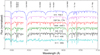 |
Fig. 1. Spectra of the cool stars observed in the field of NGC 6649. With the only exception of S19, observed with ISIS, these stars were observed with FEROS (we note the gap between orders 37 and 38 around 8540 Å). |
NGC 6664. We observed 16 stars in the cluster field. Most of them, that is, 11 of them are B stars ranging types from B2 to B9. The five remaining stars are evolved objects: the Cepheid EV Sct and four GK red (super)giants, namely S51, S52, S53, and S54. Figure 2 displays their spectra. Among the B stars, we found two Be stars (S56 and S228). McSwain et al. (2009), found five Be stars in this cluster from spectroscopic observations focused around the Hα line. Two of them, S56 and S61, were also observed by us. The first star, S56, exhibits emission in our spectrum while the other one, S61 does not. It is important to remember that our spectra do not cover Hα, but Hβ instead. S61 might still show emission only around Hα. Nevertheless, in a previous study, McSwain & Gies (2005), using Hα photometry, also found no emission in this star. The other Be star identified in this work, S228, was already included in the catalogue of Be stars from Stephenson & Sanduleak (1977), labelled as number 401.
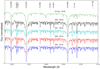 |
Fig. 2. HERMES spectra for cool stars in the field of NGC 6664 (we note the gap between orders 41 and 42 around 8580 Å). |
Be 55. In this case, we observed 12 stars, out of which five are B-type stars. These stars are among the earliest in the cluster, with spectral types in the range B4–B6. None of them exhibit an emission profile in the Balmer lines. The remaining seven stars are cool objects with spectral types comprised between G8 and M2, all of them classified as supergiants.
4.2. Cluster membership
Identifying the members associated with a cluster among all the stars present in the field is essential to characterising the cluster. Astrometry is an efficient tool for performing this disentanglement. Gaia is beginning to revolutionise astronomy by providing the most accurate astrometry for the largest number of objects to date. Based on the DR2 data, Cantat-Gaudin et al. (2018) studied a large sample of Galactic open clusters, assigning the membership probabilities for thousands of stars. In this work, we analysed the aforementioned clusters while taking into account the members found by Cantat-Gaudin et al. (2018), paying special attention to the evolved stars. The membership of all stars observed in this work are summarised in Table A.1.
NGC 6649. In this cluster, Mermilliod et al. (2008) observed five evolved stars: three RSGs (S42, S49, and S117) and two YSGs (S19 and the Cepheid, S64). All of them, with the exception of S42, are bona-fide members. This star, as already noted by Madore & van den Bergh (1975), is a double object composed of a blue (S42 B) and a red star (S42 K). The latest is the one observed by Mermilliod et al. (2008). The membership of S42 B has also been discarded, which can be deduced from the photometry (see Fig. 3) since, despite having the latest spectral type among the blue stars, it is the brightest one. Finally, the astrometry of the coolest target observed, S111, is not compatible with membership (as neither is its RV).
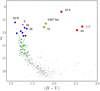 |
Fig. 3. V/(B − V) diagram for all stars in the field of NGC 6649. Stars with only BV photometry are represented by gray dots whereas those observed also in the U band appear as green dots. Stars for which we additionally have spectra are plotted with small blue circles (B-type stars), magenta diamond (Be star), and big circles: greenish-yellow for YSGs and red for RSGs. The numbering for the most representative stars is marked as well. |
NGC 6664. In this case, five evolved stars were also observed by Mermilliod et al. (2008): the Cepheid EV Sct (S80) and four RSGs, namely S51, S52, S53, and S54. According to Cantat-Gaudin et al. (2018) only S51, S52, and S80 are likely members. In addition, the colour-magnitude diagram (CMD) shows a star, BD-08 4641, which might be a new YSG member (see Sect. 4.3.2).
Be 55. This cluster was not observed by Mermilliod et al. (2008) but Negueruela & Marco (2012) found in it seven evolved stars. Six of them, S1, S2, S3, S4, S6, and S61, are RSGs while the remaining one, S5, is a YSG (the new Cepheid discovered by Lohr et al. 2018). The Gaia DR2 astrometry confirms the membership of all these stars, solely with the exception of S61, the coolest object observed in the cluster field.
4.3. Colour-magnitude diagrams
In order to determine accurate ages for our clusters, we combined archival photometry with the spectroscopy obtained in this work. As a first step, we constructed, for each cluster, CMDs in different photometric systems, highlighting the stars for which we have spectra. For both optical and 2MASS photometry, we plot the dereddened CMDs, that is, MV/(B − V)0 and MKS/(J − KS)0, respectively, whereas for the Gaia DR2 photometry, we represented the G/(GBP − GRP) CMD reddening the isochrone instead. Then, in a second step, we drew PARSEC isochrones (Bressan et al. 2012) computed at the corresponding metallicity found in Sect. 4.5.2. With the aim of ensuring the reliability of the fitting, we selected only those stars from Cantat-Gaudin et al. (2018) with a sufficiently high membership probability (i.e., P ≥ 0.7).
4.3.1. NGC 6649
We performed an analysis of the CCD photometry from Walker & Laney (1987) since the one from Hoyle et al. (2003), despite being more up-to-date, is not publicly available. It covers a field of  around the nominal cluster centre, with a magnitude limit V ≈ 20. There is BV photometry for 395 stars, out of which 82 are also observed in the U band. This photometry does not provide any data for certain interesting stars such as S52, S111, the Cepheid, and the components of the binary S42, which is the brightest in the cluster field. For the last three, we included their values, taken from Madore & van den Bergh (1975), in our sample after rescaling the photoelectric UBV values and taking into account the offset between both photometric datasets.
In the first place, we plot the V/(B − V) diagram, additionally highlighting the stars observed spectroscopically (Fig. 3). To deredden the cluster stars, we followed the procedure employed in Alonso-Santiago et al. (2018), based on the classical extinction-free Q parameter (Johnson & Morgan 1953). Since this parameter is defined as Q = (U − B)−X(B − V), we used only those stars with photometry also in the U band. From six B-stars without any peculiarities (see Table 2), we found a mean reddening of E(B − V) = 1.43 ± 0.09 and determined an average ratio X = 0.79 ± 0.04, a value that is slightly different to the standard value, X = 0.72 ± 0.03 (Johnson & Morgan 1953). With this value, we computed the Q index for selecting intrinsically blue stars in the field and assigned them photometric spectral types. We checked the validity of this spectral classification by comparing, when possible, the photometric types with those directly observed from spectra. We found consistency between both classifications within one spectral subtype.
Colour excesses for B-type stars in the field of NGC 6649.
Based on these spectral types and the positions of the stars on the V/(B − V) diagram, we selected the likely cluster members, 44 in total. From the Q index for all photometric cluster members, we estimate a mean reddening for this cluster of E(B − V) = 1.39 ± 0.06, which is compatible within the errors with that previously estimated from spectra. For the evolved population, in order to correct the reddening, we followed the procedure described in Fernie (1963), which is more specific for this type of (super)giants. Once we had completed the member selection, we estimated the cluster distance by a visual zero-age main-sequence (ZAMS) fitting. The distance modulus obtained is μ = V0 − MV = 11.15 ± 0.15, corresponding to a distance of d = 1.70 ± 0.12 kpc. The error involves the uncertainty when considering the ZAMS as a lower envelope. Our estimate, which is the result of the photometric analysis, is consistent with that derived (2.0 ± 0.4 kpc) from the Gaia DR2 parallax (0.467 ± 0.087 mas, according to Cantat-Gaudin et al. 2018, where the error represents the dispersion of individual parallaxes among members). When converting the parallax into distance, the correction proposed by Lindegren et al. (2018), involving the addition of 0.029 mas to the published value with the aim of counteracting the zero-point offset of the Gaia DR2 parallaxes, has been taken into account. Once reddening and distance have been fixed, we can proceed to determining the cluster age. For this task, we carefully fitted by eye different isochrones on the MV/(B − V)0 diagram. The best-fitting isochrone (see Fig. 4) yields a log of τ = 7.8 ± 0.1, which is equivalent to an age of 63 ± 15 Ma. In this case, the error reflects the interval of isochrones that gives a good fit. All stars fit the isochrone rather well. Only S9, an extreme Be star, lies further away. In addition, this object is an X-ray source and it is a candidate blue straggler star (BSS, Marco et al. 2007). In addition, the position of S28, already reported as a Be star by Madore & van den Bergh (1975), means it may be suspected of being another BSS, although this location might also be conditionated by its Be nature. In Fig. 4, we also plot the 2MASS KS/(J − KS)0 and Gaia DR2 G/(GBP − GRP) diagrams, obtaining a result that is analogous to that derived from the optical CMD. In these diagrams, the 484 objects found with the highest probability of membership (P ≥ 0.7, according to Cantat-Gaudin et al. 2018), have been added, together with their 2MASS counterparts, to the stars observed spectroscopically in this work. We note the presence of star 2MASS J18335423-1019100 (green triangle in Fig. 4) in the evolved region on the diagrams, which is brighter than Cepheid V367 Sct (Ks = 6.2). This object is located 8.4′ away from the nominal cluster centre and this is reason it was not covered by the optical photometry.
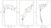 |
Fig. 4. Colour-magnitude diagrams for likely members of NGC 6649 in three different photometric systems: Left: MV/(B − V)0 from the optical photometry taken by Walker & Laney (1987); centre: MKS/(J − KS)0 (2MASS photometry); and right: G/(GBP − GRP) (Gaia DR2 data). Grey dots are the photometric data for likely members. Stars observed spectroscopically are represented as red circles (RSGs), greenish-yellow circles (YSGs), blue circles (blue stars), and magenta diamonds (Be stars). The black line shows the best-fitting PARSEC isochrone (log τ = 7.8). Star 2MASS J18335423-1019100, a possible new evolved member, is highlighted as a green triangle. |
4.3.2. NGC 6664
In the case of this cluster, we resorted to BV photometry from the APASS catalogue (DR9, Henden et al. 2016) because that of Hoyle et al. (2003) is not publicly available. In order to estimate the cluster reddening, we averaged the individual values of the blue stars (without emission lines) observed spectroscopically. By comparing the (B − V) colour for each star with the one displayed in the calibration of Fitzgerald (1970) according to its spectral type, we obtained the individual reddenings (Table 3). The mean value, E(B − V) = 0.77 ± 0.05, is compatible within the errors with the previous estimates (see Sect. 2.2). In addition, this value is also compatible with that derived by using the calibration of Straižys & Lazauskaitė (2009) from 2MASS photometry. In this case, we obtained E(J − Ks) = 0.36 ± 0.03, which is equivalent to E(B − V) ≈ 0.72. Taking this value into consideration, we plot the CMDs from the stars observed by us together with the 180 high-probability members (with their APASS and 2MASS counterparts) found in the list of Cantat-Gaudin et al. (2018). The best fit, displayed in Fig. 5, corresponds to a distance modulus, μ = 11.25 ± 0.15 (i.e., 1.78 ± 0.12 kpc), compatible within the errors with the value derived by Cantat-Gaudin et al. (2018, d = 2.0 ± 0.2 kpc), and an age of log τ = 7.90 ± 0.10 (i.e., 79 ± 18 Ma). In this diagram, all likely members lie on the isochrone. However, it is worth noting the spread around one magnitude observed among the blue stars at the top of the MS. This fact could indicate the existence of a variable reddening across the field.
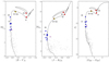 |
Fig. 5. Colour–magnitude diagrams for likely members of NGC 6664. Colours and symbols are the same as those in Fig. 4. The black line shows the best-fitting PARSEC isochrone (log τ = 7.90). Star BD-08 4641, a good candidate to be a new YSG cluster member, is highlighted as a brown square that is very close to the Cepheid EV Sct. |
Colour excesses for B-type stars in the field of NGC 6664.
As in the previous cluster, the presence of three BSS candidates in the field of NGC 6664 is reported in the literature (Schmidt 1982; Ahumada & Lapasset 1995). Only two of them, S55 and S61, are likely members and their positions are displayed on the diagrams. This issue is discussed in more detail in Sect. 5.3. Additionally, we note that the position on the CMDs of two objects suggests that these might be new evolved members. The first one is the star BD-08 4641. Since it is located at almost the same position as the Cepheid it is likely to be a new YSG member. The second candidate is the object TYC 5691-1067-1. On the CMDs, it occupies a location below S51 (see Fig. 5) in the reddest part of the diagrams. However, it is not as close to the isochrone as would be expected from a bona-fide member. In addition, both stars are placed away from the cluster centre (16.2′ and 20.2′, respectively).
4.3.3. Be 55
This cluster was already observed by our group (Negueruela & Marco 2012). From the analysis of UBV photometry, we identified 138 likely members for which we computed their reddening. Among these, half of them are bona-fide members, according to the criteria from Cantat-Gaudin et al. (2018). By averaging their individual reddenings, we obtained the value for the cluster, E(B − V) = 1.81 ± 0.15. Given its large dispersion, it is reasonable to assume the existence of a non-negligible differential reddening in the field. We constructed the CMD while taking into account the evolved objects too. For one of them, S1, our photometry did not provide any data, so we took the values given by Maciejewski & Niedzielski (2007) for this star, after correcting them from the average differences existing between both photometric datasets. In Fig. 6, from 107 high-probability members, the optical (left), 2MASS (centre), and Gaia DR2 (right) CMDs are displayed. The best-fitting isochrone, computed at [Fe/H] = +0.07 (the value found for the Cepheid, Lohr et al. 2018), corresponds to a log τ = 7.80 ± 0.10, which is equivalent to a cluster age of 63 ± 15 Ma, and a distance of μ = 12.55 ± 0.15 (i.e., 3.24 ± 0.22 kpc), which is consistent with that obtained by Cantat-Gaudin et al. (2018, i.e., 3.0 ± 0.8 kpc) from an average cluster parallax of 0.309 ± 0.091 mas. On the one hand, blue members lie on the isochrone in the three CMDs and, given the position of S7, it appears to be a BSS candidate. On the other hand, evolved stars do not show a good fit: their location does not agree with their spectral types; all of them are displaced to the left with respect to the expected position. This is surely an effect of the strong reddening present in the field (AV ≈ 5.5 mag.), which makes it difficult to correct properly for the evolved members. This effect is more important in the optical CMD (despite the correction followed from Fernie 1963) than in the 2MASS CMD, which is less sensitive to the reddening. Since it is also visible in the Gaia DR2 CMD, in which the isochrone (and not the stars) was automatically reddened, it seems that the reddening derived from blue stars is not the problem. Another possible explanation could come from the metallicity. It is well known that the lower the cluster metallicity, the warmer its evolved stars. In order to test this possibility we looked for isochrones with different metallicities, finding that a value of [Fe/H] ≈ − 0.4 yields the one that matches the position of the evolved stars better (see Fig. 6). However, according to its Galactocentric position (RGC ≈ 8.5 kpc), this value does not seem to be very reliable and, therefore, the reddening appears to be the most probable cause.
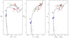 |
Fig. 6. Colour-magnitude diagrams for likely members of Be 55. Colours and symbols are the same as those in Fig. 4. The solid line shows the best-fitting PARSEC isochrone (at the Cepheid metallicity) whereas the dashed line corresponds to that computed at [Fe/H] = −0.4 (see text for details). |
4.4. Size and mass of the clusters
With the aim of determining the size of the clusters in the study, we resorted to Gaia DR2 data. Since it is an all-sky survey, it allows us to inspect not only the central part of the cluster but also its surroundings, which gives us the possibility to investigate its extent. We started our analysis by selecting the Gaia DR2 sources inside a radius of 30′ around the nominal cluster centre. Due to the huge number of objects retrieved, we modified our selection to keep only those objects with better astrometry (i.e., a parallax error smaller than 0.15 mas). In a first step, we calculated the position of the cluster centre. We assumed that this is the region where the stellar density is higher. In this way, we found it as the peak of the Gaussian corresponding to the fitting of the density profile observed along each equatorial coordinate. In a second step, we determined the stellar projected distribution by counting stars in concentric annuli around the new centre. Then we fitted this density profile to a classical three-parameter King-model (King 1962), obtaining the cluster size in terms of the core and tidal radii. The first one is defined as the radial distance at which the density becomes half of the central value, whereas the latter refers to the distance at which the cluster is diluted in the stellar background.
The region in the sky where each cluster is located as well as the properties of the cluster itself determine how it stands out from the field. In order to facilitate the identification of the cluster, we payed attention to the distribution of the brightest stars in the field (i.e., G ≤ 16), which often serve as useful as tracers of the cluster boundary. In addition to it, we also examined the arrangement of stars with a similar astrometry to cluster members, that is, those objects that in the astrometric space (ϖ, μα*, μδ) that are within a 3σ radius around the cluster centre reported by Cantat-Gaudin et al. (2018). Our results, namely, the coordinates of the centre and radii (in both angular and physical units), are displayed in Table 4. We note that NGC 6649 and Be 55 are compact clusters that are easily distinguishable from the field. Significant differences with the nominal centres were not found: (this work−nominal), Δ(α, δ) = (1.7s,−12.2″) for NGC 6649, and Δ(α, δ) = (2.4s,−8.6″) for Be 55. However, in the case of NGC 6664, the opposite is true. The cluster does not stand out from the environment and, therefore, its characterisation becomes more complicated, which leads to larger uncertainties. In this case, a difference is observed with respect to the nominal centre of Δ(α, δ) = (11.3s,−80.2″), which is considerably further than the previous values. Figure 7 shows the King profiles fitted for each cluster indicating the position of the core and tidal radii. We discuss this further in Sect. 5.1.
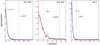 |
Fig. 7. Projected density distribution around the clusters studied in this work. Red circles are the observed values together with the Poisson errors whereas the blue line shows the fitted King profile. Vertical dashed lines represents the core (rc) and tidal (rt) radii while the horizontal one is the background density. |
Equatorial coordinates (J2000) for the centre and core (rc) and tidal (rt) radii for the studied clusters.
Once the size of the cluster is set, its mass can be inferred by integrating the initial mass function (IMF, Kroupa 2001). This procedure was followed in past analyses of other clusters (a more detailed explanation is presented in Alonso-Santiago et al. 2018). To calibrate the IMF, we need to know the number of stars located inside the cluster limits that are within a certain mass range. In this range, completeness must be assured. The best approach to do this is by counting the brightest blue stars located at the top of the MS. Our selection spans the whole B spectral type starting from the earliest type observed at the turn-off point (TO), B5–B6 in these clusters. From the Gaia DR2 CMD, we determined the average G magnitude for these stars (GTO) together with the individual dispersion around it. Based on the differences in magnitude and mass among the B spectral types (according to Straižys 1992), and considering the similarity between the G and V bands, we obtained the magnitude range to cover stars from the TO down to spectral type B9 V (whose average mass is 2.6 M⊙). Then, once the calibration of the IMF was done, its integration allowed us to obtain an estimate of the cluster mass. Taking into account these assumptions, this is only an approximate value. The numbers for each cluster are as follows:
NGC 6649. We find a GTO = 12.6 ± 0.2 for a spectral type B5 V (4.8 M⊙). We cut at G = 14.1 to reach B9 stars. In total, in this range, we counted 57 stars. This implies a present mass around 1800 M⊙, equivalent to an initial mass ≈2600 M⊙.
NGC 6664. In this case, we find a TO around B5–B6 V, with an average GTO = 12.2 ± 0.5. From 61 stars (down to G = 13.9), we inferred a present mass of around 2000 M⊙ and an initial value of 2900 M⊙.
Be 55. This is the least massive cluster. Only 24 stars are observed between B6 V (at GTO = 14.9 ± 0.1 and 4.1 M⊙) and B9 V (G = 16.0). This number implies a mass of 900 M⊙ for the present and ≈1300 M⊙ for its birth. We come back to this cluster in Sect. 5.1.
4.5. Spectroscopic analysis
4.5.1. Radial and rotational velocities
For the cool stars (observed at high resolution), before computing the atmospheric parameters and the chemical abundances, we need to prepare their spectra. In a first step, we corrected them for the RV. We determined the heliocentric radial velocity through Fourier cross-correlation by employing the ISPEC software (Blanco-Cuaresma et al. 2014). For each target spectrum, the cross-correlation was computed against a list of atomic lines masks selected for the Gaia benchmark stars library pipeline based on asteroids observed with the NARVAL spectrograph.
NGC 6649. For this cluster we obtained the mean RV from the two red (super)giants (i.e., S49 and S117) since the RV of the Cepheid is somewhat different from those stars (probably due to its variability, as this number, derived from a single epoch, only represents a random point of its radial velocity curve). Our value, vrad = −8.66 ± 1.03 km s−1, is in perfect agreement with −8.59 ± 0.40 km s−1, the value computed by Mermilliod et al. (2008) from five stars (including the Cepheid and the non member S42 K). The non-membership of S42 K and S111 (see Table 7) is confirmed also based on a RV criterion.
NGC 6664. EV Sct shows a noisy double-peak CCF, despite it not being a binary object (as noted above in Sect. 2.2). This fact prevents us from carrying out a reliable analysis of its spectrum, which is the reason this star is not taken into account to estimate the cluster average. Among the remaining evolved stars, S51 and S52, we calculated the RV for the cluster, vrad = 19.34 ± 0.21 km s−1. This value is compatible, within the errors, with the value obtained by Mermilliod et al. (2008, 18.58 ± 0.69 km s−1).
Be 55. The resolution at which we observed the stars of this cluster does not allow us to perform the spectroscopic analysis, but it is enough to estimate their RVs from the IDS spectra (those with the highest resolution available in our sample, displayed in Table 5). We obtained a (weighted) average value for the cluster, vrad =−31.7 ± 7.4 km s−1. As shown, the error (calculated as the dispersion of individual measurements) is quite large, since RVs for bona-fide members are distributed in a wide range (≈ − 20–40 km s−1). Star S1 is responsible for much of this dispersion and, additionally, it is the brightest star of the cluster. This fact could hint at its possible binary nature. Disregarding this star, the average value is vrad = −27.7 ± 4.9 km s−1, whose dispersion is within twice the instrumental error (around 3 km s−1). Unfortunately, Be 55, unlike the previous clusters, was not observed by Mermilliod et al. (2008).
Radial velocites for stars in the field of Be 55.
In a second step, we estimated the contribution of rotational and macroturbulence broadenings since the former is used as an input when computing the atmospheric parameters. The projected rotational velocity (v sin i) is calculated by using the IACOB-BROAD code (Simón-Díaz & Herrero 2014). It is based on the Fourier transform method and is able to separate rotation from other broadening mechanisms such as the macroturbulent velocity (ζ). We used as a diagnostic, at least eight lines of Fe I and Ni I that are clearly visible in the spectra. The errors reflect the scatter between measurements, in terms of the root mean square (rms). All these radial and rotational velocities, for NGC 6649 and NGC 6664 are listed in Table 7.
4.5.2. Stellar atmospheric parameters
We derived the stellar atmospheric parameters for 35 objects. However, as we have done in previous works (see e.g., Alonso-Santiago et al. 2019b), depending on the temperature range of the stars, we follow one of two different procedures. Additionally, it is important to note the different resolution with which both groups of targets have been observed. On the one hand, we have low-resolution spectra for B stars, whereas on the other hand, high-resolution spectra have been taken for the cool stars.
Regarding B stars, we computed stellar parameters from their ISIS spectra for 26 stars: ten are distributed in the field of NGC 6649, 11 in that of NGC 6664, and the remaining five in Be 55. We followed the strategy described by Castro et al. (2012), employing a grid of FASTWIND synthetic spectra (Simón-Díaz et al. 2011; Castro et al. 2012) and adopting FASTWIND as the stellar atmosphere code (Santolaya-Rey et al. 1997; Puls et al. 2005). By using an automatic χ2-based algorithm, we found the stellar atmospheric parameters that best reproduce the main strong features observed in the range ≈4000 – 5000 Å. Because of the resolution of these spectra is not as high as is necessary to separate the different broadenings, we assumed a rotational origin for the whole broadening. Hence, we also calculated the rotational velocity in an interactive way. First, we chose as an initial estimate of the v sin i a value close to the resolution, that is, around 50 km s−1. Then, we computed a first model capable of reproducing the spectrum. Once the stellar parameters were fixed, we looked for a second value of rotation by changing it until we found a new model which best reproduced the profiles. We repeated this process at least a few times to make sure that the rotation did not change. Our results (i.e., effective temperature, surface gravity, and projected rotational velocity) are displayed in Table 6. The temperatures derived are in good agreement with the spectral types assigned, according to the calibration by Humphreys & McElroy (1984).
Stellar atmospheric parameters for the blue stars derived from ISIS spectra.
For cool stars, the methodology is quite different. We analysed nine stars, five observed with FEROS in the field of NGC 6649, and four others in NGC 6664 observed with HERMES. Additionally, we also tried to calculate stellar parameters for EV Sct. However, because of its double-peak CCF, we have not been able to provide reliable results. We generated a grid of synthetic spectra from LTE MARCS spherical models (Gustafsson et al. 2008) by using SPECTRUM (Gray & Corbally 1994) as a radiative transfer code. Effective temperature (Teff) ranges from 3300 K to 7500 K with a step of 100 K up to 4000 K and 250 K until 7500 K, whereas surface gravity (log g) varies from −0.5 to 3.5 dex in 0.5 dex steps. In the case of metallicity (using [Fe/H] as a proxy), the grid covers from −1.5 to +1.0 dex in 0.25 dex steps. We fixed the value of the microturbulent velocity (ξ) according to the calibration presented in Dutra-Ferreira et al. (2016). Our linelist, based on that provided by Genovali et al. (2013), contains ∼230 features for Fe I and ∼55 for Fe II.
We employed an updated version of the STEPAR code (Tabernero et al. 2018) tailored to the present problem. Our code used the Metropolis–Hastings algorithm as optimization method. It generates simultaneously 48 Markov-chains of 750 points, each performing a Bayesian parameter estimation. For this task, we resorted to an implementation of Goodman & Weare’s Affine Invariant Markov chain Monte Carlo Ensemble sampler (Foreman-Mackey et al. 2013). A χ2 function is implemented with the aim of fitting the selected iron lines. The stellar rotation and the instrumental broadening are fixed to the value previously derived for the former (Sect. 4.5.1) and the resolution of the spectrographs, respectively. The macroturbulent broadening was left as a free parameter in order to absorb any residual broadening.
For the M supergiant in NGC 6649, S111, we were forced to change our methodology. It is known that the spectrum of M stars is dominated by molecular bands that erode the continuum and, therefore, identifying a large number of spectral features becomes very difficult, if not impossible. However, these bands are very useful since their depth is very sensitive to temperature (García-Hernández et al. 2007). Based on this suggestion, we paid attention to the region 6670–6730 Å, where the TiO bands at 6681 Å and 6714 Å are clearly present. For this star, we computed its stellar parameters based on a χ2-minimisation code, with the same grid of MARCS synthentic spectra, which we previously described, but using TURBOSPECTRUM (Plez 2012) as a transfer code.
Results (i.e., effective temperature, surface gravity, macroturbulent velocity, and iron abundance) are displayed in Table 7. From the analysis of the confirmed evolved members, we estimated a solar average metallicity for these clusters. In the case of NGC 6649, from stars S49, S117 and V367 Sct, we computed a [Fe/H] = + 0.02 ± 0.07, calculating it as a weighted average and taking as error the dispersion between individual values. In the same way, for NGC 6664, from S51 and S52, we derived a metallicity, [Fe/H] = − 0.04 ± 0.10.
Stellar atmospheric parameters for the cool stars derived from high-resolution spectra.
4.5.3. Chemical abundances
We only derived chemical abundances for the cool stars, eight in total (four in the field of NGC 6649 and four others in NGC 6664) since a high spectral resolution is required for this sort of study. Once we set the atmospheric parameters, it is almost trivial to derive the chemical abundances from equivalent widths (EWs). For most of the elements analysed, namely, Na, Mg, Si, Ca, Ti, Ni, Y, and Ba, we measured the EWs using TAME (Kang & Lee 2012) in a semi-automatic fashion. Instead, for lithium and oxygen, which are more delicate elements, we measured the EWs by hand with the IRAF SPLOT task. For the former, we employed a classical analysis using the 6707.8 Å line, taking into account the nearby Fe I line at 6707.4 Å. We expressed this abundance in terms of the standard notation, namely, A(Li) = log [n(Li)/n(H)] + 12. In the case of oxygen, we followed the procedure described in Bertran de Lis et al. (2015), focusing on the [O I] 6300 Å line and keeping in mind that it is blended with a Ni I feature. Finally, based on the methodology explained in D’Orazi et al. (2013), we computed rubidium abundances performing stellar synthesis for the 7800 Å Rb I line.
Results are displayed in Table 8 for the stars in the field of NGC 6649 and in Table 9 for NGC 6664. We estimate the cluster average by using the weighted arithmetic mean (employing the variances as weights) taking only the members into account. The error averages the typical individual error and the star-to-star dispersion. In both clusters, members share a similar chemical composition. However, in NGC 6649, V367 Sct exhibits a Na abundance around 0.7 dex higher than the other cluster giants. Also, S117 shows high abundances of Ca and Ni. On the other hand, the largest differences found for members of NGC 6664 (for O and Si) are around 0.4 dex.
Chemical abundances, relative to solar abundances by Grevesse et al. (2007), measured on the cool stars in the field of NGC 6649.
Chemical abundances, relative to solar abundances by Grevesse et al. (2007), measured on the cool stars in the field of NGC 6664.
5. Discussion
In this work, we present spectroscopic observations of the largest number of stars in the fields of NGC 6649 and NGC 6664 thus far. We combine our spectra with archival photometry and Gaia DR2 data in order to perform a consistent photometric analysis and properly determine the parameters of each cluster. For the first time, we have derived stellar atmospheric parameters for both blue and evolved members as well as the chemical abundances for the latter (but only for NGC 6649 and NGC 6664 stars).
5.1. Cluster parameters
In this work, we conduct a comprehensive analysis of NGC 6649, NGC 6664, and Be 55 and we summarise their properties in Table 10. We find that the distance of the clusters derived from the photometric analysis (dZAMS in Table 10) is consistent with the one corresponding to their Gaia DR2 parallaxes (dGDR2). We conclude that these three clusters are coeval, younger than the Pleaides, with an age of ≈70 Ma, which is in good agreement with the earliest blue members found, with spectral types around B5–B6. The age of Be 55 (63±15 Ma) agrees with the result of Molina Lera et al. (2018, 30–100 Ma) and it is compatible within the errors with Negueruela & Marco (2012, 50 ± 10 Ma). In addition, our value is also consistent with that of the Cepheid obtained from a different approach (Lohr et al. 2018, 63 Ma). According to the isochrones, at the age of these clusters, the mass of the (super)giants is supposed to be ≈6 M⊙, with an uncertainty of around 0.3 M⊙. This value evaluates the difference of mass found when propagating the uncertainty associated with the choice of the isochrone.
Summary of the parameters derived in this work for the clusters in this study.
As previously noted (Sect. 4.5.1), our RVs are consistent with those of Mermilliod et al. (2008). The average RVs calculated for NGC 6664 and Be 55 are fully compatible with those expected in the line-of-sight direction for each cluster according to the Galactic rotation curve (Reid et al. 2014). However, this is not true for NGC 6649, which, despite being very close to NGC 6664 in the sky (separated by only 2.3°) and at similar distances (≈2 kpc), shows a RV that is quite different (−8.7 and +19.3 km s−1, respectively). Therefore, NGC 6649 seems to have a peculiar RV, which is unexpected since it is young enough to act as a good tracer of its birthplace. Recently, Soubiran et al. (2018), based on Gaia DR2 RVs, recalculated the RVs for hundreds of open clusters, including our targets. For NGC 6649, they provide a RV = −8.87 ± 0.92 km s−1 by using four stars, in addition to −4.44 (NGC 6664, only one star) and −43.58 ± 9.24 (Be 55, four). These values are merely indicative since the same stars have not always been considered members by the different authors, making their comparison less reliable. For NGC 6649, the three values (including the result of Mermilliod et al. 2008) show an excellent agreement. In the case of NGC 6664, Soubiran et al. (2018) estimated a value smaller than ours, which approximates it to that of NGC 6649 (using only one star). In addition, for Be 55 their value is compatible, within the errors, with ours because the dispersion is very large, although our value (derived from a larger sample) is smaller. Although the potential of Gaia is huge in this field, at present, the current DR2 still does not provide enough values to properly sample open clusters. Over the next few years, upcoming DRs will shed light on this topic, also allowing for a better understanding of Galactic dynamics.
From a simple visual inspection of the sky region around the nominal centre of each cluster, we can already get a first impression of their relative appearance. In an increasing size order, we find Be 55 (with a diameter around 2–3′), NGC 6649 (≈5′) and NGC 6664 (a more diffuse cluster that seems to extend up to 7–10′). This trend is shared by the different studies found in the literature. Beyond this fact, results from different papers are not directly comparable since the variables computed to characterise the cluster size are somewhat different in each case. In Table 11, we compare our results to those obtained in recent large surveys. Kharchenko et al. (2013), from the PPMXL and 2MASS data, obtained angular and physical values for both the core (r0 and rc) and limiting radii (r2 and rt). Since the distances for each cluster (ours and theirs) are different, it is more adequate to compare angular values. Results are similar for NGC 6649 and Be 55, but in the case of NGC 6664, our values are significantly larger (since it does not stand out from the field). Sampedro et al. (2017, Sam17 in Table 11), based on astrometry from the UCAC4 catalogue, yielded numbers for the radius very similar to those of Cantat-Gaudin et al. (2018, CG18). Authors of the latter work, by analysing Gaia DR2 data, provided the radius (r50) within which half of the members that have been identified are contained. The values from these authors, as expected, are comprised between the core and tidal radii that we calculated. Finally, Maciejewski & Niedzielski (2007) investigated Be 55 and found a very compact cluster (rc = 0.7 ± 0.1 ′) with a limiting radius of 6′.
Comparison of the cluster sizes (arcmin) derived in this work and in the literature.
Regarding the mass of these clusters, in spite of our rough estimates, we find that NGC 6649 and NGC 6664 are moderately massive clusters with initial masses around 2500–3000 M⊙ which host at least three (super)giant stars, which is in good agreement with what is expected from simulations (see discussion in Negueruela et al. 2018). However, among the three clusters investigated in this paper, Be 55 hosts the largest number of evolved stars, despite being the smallest and least massive cluster. This evidence could be attributed to the fact that the lower brightness of the stars in this cluster (roughly 2.5 magnitudes fainter than those in NGC 6649 NGC 6664) has made it difficult to select the members, leaving out a (large?) number of potential candidates. Our value for its present mass, ≈900 M⊙, is slightly larger than that obtained by Maciejewski & Niedzielski (2007, 795 M⊙). In this age range, open clusters containing a similar number of (super)giants are rare (see Table 15) and also significantly more massive. Representative examples of this kind of clusters are NGC 6067 (Alonso-Santiago et al. 2017), Be 51 (Negueruela et al. 2018), and NGC 2345 (Alonso-Santiago et al. 2019b).
5.2. Stellar parameters and abundances
The reliability of our methodology is corroborated when plotting the Kiel diagram, that is, log g/Teff (Fig. 8). In this diagram, which is independent of distance, we can appreciate how well the data which have been derived photometrically, such as the isochrone, fit the spectroscopic results that have been calculated with two different procedures for blue and cool stars, respectively. The fitting is better for the latter group since, unlike the former, it was observed at high resolution. In any case, with the only exception of the BSSs, as expected, members lie on the isochrones.
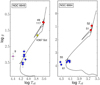 |
Fig. 8. Kiel diagram for likely members in NGC 6649 and NGC 6664. Colours and symbols are the same as those in Fig. 4. |
We obtained a solar composition for NGC 6649 ([Fe/H] = + 0.02 ± 0.07) and NGC 6664 ([Fe/H] = − 0.04 ± 0.10). As mentioned earlier in this paper, these clusters had not been, to date, spectroscopically observed at high resolution, which is reason there are no studies we could compare our results against. Instead, we resorted to the Galactic gradient and trends. Regarding the former, we took as a reference the work by Genovali et al. (2013, 2014). They estimated the radial distribution of metallicity in the Milky Way (−0.06 dex kpc−1) by employing Cepheids. They are appropriate for contrasting our results since Cepheids are young enough (τ ≈ 20 – 400 Ma) for tracing present-day abundances. In Fig. 9, we display the positions of our clusters on this gradient, including Be 55 (represented by its Cepheid, whose metallicity is [Fe/H] = + 0.07 ± 0.12). For comparison, we also overplotted some young clusters (i.e., age below 500 Ma) from the sample studied by Netopil et al. (2016) as well as some other young clusters investigated by our group. Our clusters lie below this gradient, indicating that their metallicities are lower than those expected according to their Galactocentric positions.
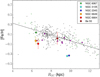 |
Fig. 9. Iron abundance gradient in the Milky Way found by Genovali et al. (2013, 2014). The black line is the Galactic gradient, green crosses are Cepheids studied in those papers, whereas black dots show data for other Cepheids from literature used by these authors. Magenta triangles represent young open clusters in the sample compiled by Netopil et al. (2016). The orange circle is NGC 6649 and the red one is NGC 6664. Finally, other clusters analysed by our group with the same technique are marked with star symbols. All the values shown in this plot are rescaled to Genovali et al. (2014), i.e., R⊙ = 7.95 kpc and A(Fe) = 7.50. |
Finally, we also compare our abundances with the Galactic trends for the thin disc (Fig. 10). We plot abundance ratios [X/Fe] vs [Fe/H] obtained by Adibekyan et al. (2012) for Na, Mg, Si, Ca, Ti, and Ni and by Delgado Mena et al. (2017) for Y and Ba in the framework of the HARPS GTO planet search program. The chemical composition of both clusters is compatible, within the errors, with the Galactic trends observed in the thin disc of the Galaxy. The [Si/Fe] ratio for both clusters and the [Ca/Fe] for NGC 6649 lie slightly above the trend, but are still consistent. The [α/Fe] ratios are slightly enhanced, presenting values of +0.19 and +0.10 for NGC 6649 and NGC 6664, respectively. We derive a roughly solar [Y/Fe] against a supersolar [Ba/Fe], which is in good agreement with the dependence on age and Galactic location found by Mishenina et al. (2013) by comparing the abundances of Y and Ba in different open clusters. Remarkably, we find a strong over-abundance of barium ([Ba/Fe] ≈ +0.8), which is in line with that described by D’Orazi et al. (2009). They studied the evolution of barium with time for dwarf stars in open clusters. They found (see their Fig. 2) the highest abundances, similar to ours, in the youngest clusters of their sample (specially for those clusters with ages τ≤100 Ma). These abundances are higher than those predicted by standard theoretical models. To explain this enrichment of Ba, D’Orazi et al. (2009) suggested the so-called “enhanced s-process”, namely, the use in chemical evolution models of a higher yield of Ba with respect to the s-process (the contribution of the r-process is not so important and its yields are only affected at low metallicity). Finally, none of these stars have the high abundances of Li and Rb that we could expect for a super-AGB, confirming their evolutionary status as massive red giants, inferred from their positions on the CMDs.
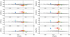 |
Fig. 10. Abundance ratios [X/Fe] versus [Fe/H]. The grey dots represent the Galactic trends for the thin disc (Adibekyan et al. 2012; Delgado Mena et al. 2017). NGC 6067, NGC 3105 and NGC 2345 are drawn with triangles (green, cyan, and blue, respectively), whereas NGC 6649 and NGC 6664 are the orange and red circles, respectively. Clusters are represented by their mean values. The dashed lines indicate the solar value. |
5.3. Blue straggler stars
The existence of BSSs in open clusters, and their relationship with the Be phenomenon, has been known for a long time (see Mermilliod 1982, and the references therein). These stars, because of their anomalous positions on the CMDs, appear to be younger than the rest of the cluster members. They seem to be brighter and bluer than the MS stars at the cluster turn-off point. Although several mechanisms have been suggested to explain the origin of the BSSs, in young open clusters the leading scenario is the mass transfer between companions in a multiple system (McCrea 1964; Perets & Fabrycky 2009).
The presence of these kind of objects is very common at this age in Galactic open clusters, as we have previously studied (see e.g., the discussions in Marco et al. 2007; Alonso-Santiago et al. 2017). In the field of the clusters investigated in this paper, five objects have been proposed as BSS candidates: S9 (Marco et al. 2007) and S35 (Ahumada & Lapasset 1995) in NGC 6649 and S55, S59, and S61 in NGC 6664 (Schmidt 1982; Ahumada & Lapasset 1995). Based on astrometry (see Table A.1), the cluster membership for S59 has been discarded. Among the remaining four, when examining our data, only S35 seems to be a normal B-type MS star. On the contrary, S9, S55, and S61 fulfill the observational conditions expected for BSS candidates. They have the earliest spectral types in each cluster and occupy peculiar positions on both the CMD and Kiel diagrams. In addition, here, we present two new mild candidates: S28 (NGC 6649) and S7 (Be 55). However, regarding the Kiel diagram, S28 occupies a normal position and for S7, the atmospheric parameters have not been calculated. Remarkably, as in the case, for example, for stars 267 and HD 145304 in NGC 6067 (Alonso-Santiago et al. 2017), the spectrum of S55 (BN2 IV) shows the enhancement of some nitrogen features, which is in good agreement with anomalies in the CNO abundances as predicted by the mass-transfer mechanism (Sarna & De Greve 1996). Morever, the fact that three of the five candidates – S9 (which is even an X-ray source), S61, and S28 – are known Be stars also supports this scenario.
5.4. Cepheids
Cepheids are surely the best-known variable stars for being primary standard candles. Since the beginning of the 20th century, is well known that their brightness is directly proportional to their period (Leavitt & Pickering 1912). However, Cepheids, beyond cosmological or extragalactic implications, are astropysical laboratories of great importance in the study of stellar evolution. Cepheids are YSGs (i.e., typically from mid-F to early-G spectral types) with masses in the range of 3–10 M⊙, whose progenitors are B-type stars of the MS. Yellow supergiants become unstable and begin to pulsate, turning into Cepheids, when crossing the instability strip (IS). Cepheids allow us to constrain evolutionary models for intermediate-mass stars, especially when they are hosted in open clusters, such as δ Cep, which is the prototype of this type of objects, in the young stellar association of Cep OB6 (Majaess et al. 2012). However, this is an unsual occurrence: despite the fact that more than 3 000 open clusters are known in the Galaxy (Kharchenko et al. 2016), only 31 contain Cepheids (Chen et al. 2017). Among them, in this paper we have focused on three targets, whose main properties are shown in Table 12. In order to minimise the possible effect that the parallax zero-point offset of the current Gaia DR2 (Groenewegen 2018) may have on our results, the distances listed below are calculated as the weighted average of the values derived from the individual parallax for each Cepheid (see Table A.1) and the cluster mean (via ZAMS fitting, Table 10). Tabulated reddenings, E(B − V), are also the average of the cluster mean and the individual values (i.e., 1.33 and 0.62 for V367 Sct and EV Sct, respectively) derived from their average BV magnitudes and the calibration of Fitzgerald (1970). Finally, for the little-studied Cepheid S5, we estimated the JHKs average values by employing the PLR obtained by Chen et al. (2017).
Summary of the parameters for the Cepheids studied in this work.
5.4.1. V367 Sct
We calculated parameters and abundances for only one of the three aforementioned Cepheids (V367 Sct). Unfortunately, we were unable to disentangle the properties of EV Sct with our current methodology due to the ambiguous profile of the lines displayed in its spectrum. In the case of the third Cepheid, S5, it could not be analysed because it had been observed at lower resolution.
Genovali et al. (2014) derived the atmospheric parameters for a large number of Cepheids, including V367 Sct. Their results, compared to ours, are displayed in Table 13. Their errors represent the standard deviation of the different values derived from individual spectra. Since Cepheids are pulsating variables, their parameters depend on the moment of the observation (especially the effective temperature), a fact that must be taken into account when comparing both sets of results. Even so, effective temperature and metallicity are compatible within the errors. However, microturbulent velocity and surface gravity are rather different. As both works use the same linelist and MARCS models, this difference might reside in the methodology employed. The cited authors computed the stellar parameters as decoupled quantities, whereas we derived them as coupled variables at the same time. According to Torres et al. (2012) this different approach to atmospheric parameters could introduce a bias into the results.
Comparison of the results obtained for the Cepheid V367 Sct from this work (TW) and Genovali et al. (2014) for the stellar atmospheric parameters and Genovali et al. (2015) for the chemical abundances, relative to solar values from Grevesse et al. (2007).
The chemical composition of the Cepheid is mostly compatible within the errors with those of the parent cluster. The only exceptions are the abundances of Na and Ca. Genovali et al. (2015) computed abundances for α-elements based on stellar parameters that were previously obtained in Genovali et al. (2014). In Table 13 we also compare their chemical abundances with ours. Both sets of abundances, including Na and Ca, are fully compatible. We note that for the Cepheids in common with Genovali et al. (2014, both here and in previous works) our results are compatible within the errors with theirs. In our case, the cluster abundances are derived from red (super)giants, whereas they used Cepheids for the Galactic gradient. This is a possible explanation for the offset observed in Fig. 9.
5.4.2. Ages and masses: Pulsating versus evolutionary values
Cluster Cepheids help us determine the cluster age when fitting isochrones since they provide an extra anchor point between the brightest blue members and the RSGs. The age thus obtained for the cluster and, therefore for the Cepheid itself, can be checked with the age inferred from the period-age relation (PAR). On the one hand, a family of PARs based on theoretical models of stellar evolution yields the pulsating age of the Cepheid from its observed period. Results depend strongly on the input physics. In order to illustrate this point, we employed a canonical PAR from Bono et al. (2005), which does not account for rotation, along with a non-canonical one from Anderson et al. (2016), which assumes an average initial rotation (ω = 0.5). On the other hand, a branch of empirical PARs also exists, having been calibrated with Cepheids hosted in open clusters, such as those of Efremov (2003) and Turner (2012). The former employed cluster Cepheids in the LMC, while the latter focused on Galactic ones. Similarly, we used a mass-luminosity relation (MLR, derived by Anderson et al. 2014) to estimate the pulsating masses of the Cepheids from their average V magnitudes (⟨V⟩). Luminosities were calculated assuming individual distances (Table 12), bolometric corrections for supergiants given in Humphreys & McElroy (1984), and an absolute bolometric magnitude for the Sun,  . In Table 14, we compare the pulsating ages and masses calculated in this way with those values inferred from the isochrones.
Age (Ma) and mass (M⊙) of cluster Cepheids derived from their parent cluster (inferred from isochrones) and by using different period-age (PAR) and mass-luminosity (MLR) relations.
The differences in the results from both model-based PARs cannot be attributed exclusively to the effects of rotation. Although both PARs are computed for fundamental and first overtone modes Cepheids at the Galactic metallicity (ZMW), they use different values for it: ZMW = 0.02 (canonical) and ZMW = 0.014 (non-canonical model). In addition, the first one takes into account all the evolutionary phases inside the IS whereas the non-canonical PAR is only valid for second and third IS crossings. Evolutionary ages derived from isochrones are in excellent agreement with the canonical PAR of Bono et al. (2005) since the rotating PAR gives older (unrealistic) ages, which are not compatible with the stellar B-type population observed in these clusters. Concerning the empirical PARs, which are not specific to the pulsation mode or the IS crossing number, they yield older ages than that of Bono et al. (2005). The PAR of Turner (2012) gives realistic numbers (with the exception of EV Sct), whereas the estimates obtained from the relation of Efremov (2003) are very similar to those derived from the rotating PAR. Regarding the mass, although a mass discrepancy would be expected (Anderson et al. 2014), both approaches provide a similar value.
5.4.3. YSG/RSG ratio
Throughout the life of Cepheids, IS crossing occurs on up to three occasions3: the first one before the first dredge-up (in the H-shell burning phase) and the other two take place during the blue loop (He-core burning phase), where they spend most of their lifetimes as Cepheids (Anderson et al. 2014). The Cepheids/RGs ratio we observed is very sensitive to the extension of the blue loop, which strongly depends on metallicity and the input physics assumed by the theoretical models (Matraka et al. 1982; Ekström et al. 2012; Anderson et al. 2014; Walmswell et al. 2015). According to this, in order to check theoretical predictions with observations, in our previous paper, we looked in the literature for young open clusters that host Cepheids. As we only found a dozen, we decided to enlarge our sample to make it more representative and to include all the clusters with ages between 50 and 100 Ma observed by Mermilliod et al. (2008), in addition to counting all the YSGs, not only Cepheids (for a detailed description, see Alonso-Santiago et al. 2017). In this way, we calculated a yellow-to-red (super)giants ratio, YSG/RSG = 0.19. According to Ekström et al. (2012), at solar metallicity, we estimated that this ratio was expected to be around YSG/RSG ≈ 0.6 (considering models with and without rotation), which is in good agreement with Matraka et al. (1982), in the case where they included a moderate overshoot in the models. Therefore, the observed value was lower than those predicted by stellar evolutionary models.
As seen before (Sect. 4.2), in light of Gaia DR2 astrometry, we have had to discard the membership of some (super)giants which, to date, were assumed to be bona-fide members according to their positions on the respective CMDs and their RVs that are compatible with the cluster value (Mermilliod et al. 2008). To check the impact that these false members may have had on our previous study, we have reviewed all the clusters in our sample (Alonso-Santiago et al. 2017) to consider the membership of each star according to the probabilities estimated by Cantat-Gaudin et al. (2018). The new values are displayed in Table 15. In total, we examined 54 clusters (with ages in the 50–100 Ma range), finding 89 RSGs and 18 YSGs, which represents a YSG/RSG ≈ 0.2, which is the same result as the one previously obtained and also compatible with younger clusters, such as NGC 3105 (Alonso-Santiago et al. 2018). Consequently, our previous inference remains valid: in the domain of intermediate-mass stars, theoretical models predict a higher YSG/RSG than the ratio observed in young open clusters. Additionally, the disagreement between theoretical predictions and observations also becomes evident when considering the unexpected positions of the Cepheids on the CMDs. According to Anderson et al. (2014), almost all Cepheids (≈99%) should be observed during their passage through the blue loop. Nevertheless, it is noticeable that this is not what we are seeing in these clusters given two of the three Cepheids are crossing the Hertzsprung gap.
Number of red (super)giant stars and yellow supergiants, (Cepheids or not, in brackets) in open clusters with ages between 50 and 150 Ma (from Mermilliod et al. 2008).
6. Conclusions
In this work, we observe three young open clusters, namely NGC 6649, NGC 6664, and Be 55, which share an unusual property: each of them is host to a Cepheid. We collected the largest spectroscopic sample of these clusters to date. For each of the clusters, we compiled a list of preferred members by selecting only the high-probability members according to Cantat-Gaudin et al. (2018), whose selection was based on Gaia DR2 astrometry. Then, in conjunction with our observations, we reanalysed archival photometry in the context of our list. As a result of these analyses, we placed the clusters at distances compatible with those inferred from their Gaia DR2 average parallaxes, ultimately placing NGC 6649 and NGC 6664 slightly below 2 kpc and Be 55 somewhat further, above 3 kpc. We also determined accurate ages for these clusters, with similar values around 70 Ma, which are in good agreement with the spectral type found for the earliest blue stars, around B5–B6. At this age, the mass of the evolved stars are roughly 6 M⊙ in the massive range of the intermediate-mass stars. We also computed the size of these clusters, estimating their initial masses to be in the range 1000–3000 M⊙. In addition, we confirmed the presence of two BSSs in NGC 6649 and one in NGC 6664, along with arguing a claim for two other mild BSS candidates (in NGC 6649 and Be 55, respectively).
The accuracy and broad availability of Gaia DR2 astrometry could have a certain impact on the study of open clusters. Upcoming data releases are expected to fix offsets and systematics that will allow us to improve our knowledge in this field. Changes in the membership status of some evolved members that are not very numerous in this age range could modify cluster parameters, such as age in the process of fitting isochrones. For NGC 6664, we discarded the membership of two of the four known RSG members. However, we find a likely candidate to be a new YSG member, star BD-08 4641, whose astrometric properties as well as its position on the CMDs are fully compatible with cluster membership. Future spectroscopic observations should be of great help to confirm this assumption.
For the first time, atmospheric stellar parameters have been computed for stars in NGC 6649, NGC 6664, and Be 55. For the first two clusters, we analysed both hot and cool stars, whereas for the third one, Be 55, we only studied blue members. The procedure followed in our investigation has proven to be robust since parameters obtained for both sets of stars using different codes and techniques agree quite well, as shown in the Kiel diagrams. The positions of the stars in these diagrams (derived from the spectroscopic analysis) properly lie on the isochrones (which correspond to the photometric ages).
In addition, for the first time, we studied the chemical composition of NGC 6649 and NGC 6664 from their evolved stars. We have determined chemical abundances of Li, O, Na, α-elements (Mg, Si, Ca, and Ti), the Fe-group (Ni), and s-elements (Rb, Y, and Ba). Both clusters show a solar composition ([Fe/H] = +0.02 ± 0.07 and [Fe/H] = −0.04 ± 0.10, respectively) but they are slightly metal-poor relative to the mean of the Galactic gradient. They exhibit a mild α-enhancement ([α/Fe] = +0.19 and [α/Fe] = +0.10, respectively) and a chemical composition compatible with the trends observed in the Galactic thin disc. As expected for RGs which have not yet begun the AGB phase, none of the evolved stars show representative abundances of either Li or Rb. However, we have found a significative overabundance of Ba ([Ba/Fe] ≈ 0.8 dex), which supports the theoretical scenario of the enhanced s-process.
Cepheids in open clusters offer us the possibility to better calibrate the PLRs for anchoring the distance ladder and, thus, contributing to a mitigation of the H0 tension. They also give us the opportunity to test evolutionary models. Observables such as the ratio of yellow to red (super)giants (effectively lower than expected) and determinations of Cepheid properties (mass and age) from the study of the parent cluster are of great importance in constraining theoretical models. The differences detected between the observations and predictions reflect the uncertainty that current evolutionary models of the most massive intermediate-mass stars still suffer from.
According to some evolutionary models (see e.g., Turner et al. 2006, for references), in some cases, a fourth and fifth crossing could occur during the He-shell burning phase, but the reality of these extra crossings has not been confirmed (Anderson et al. 2016).
Acknowledgments
We thank the anonymous referee for their helpful suggestions which have helped to improve this paper. This research is based on observations collected with the MPG/ESO 2.2-meter Telescope operated at the La Silla Observatory (Chile) jointly by the Max Planck Institute for Astronomy and the European Organization for Astronomical Research in the Southern hemisphere under ESO programme 095.A-9020(A). This research is also based on observations made with the Mercator telescope (operated by the Flemish Community) and the INT and WHT telescopes (operated by the Isaac Newton Group of Telescopes) on the islad of La Palma at the Spanish Observatorio del Roque de los Muchachos of the Instituto de Astrofísica de Canarias. Some observations were obtained with the HERMES spectrograph, which is supported by the Research Foundation – Flanders (FWO), Belgium, the Research Council of KU Leuven, Belgium, the Fonds National de la Recherche Scientifique (F.R.S.–FNRS), Belgium, the Royal Observatory of Belgium, the Observatoire de Genève, Switzerland and the Thüringer Landessternwarte Tautenburg, Germany. This research is partially supported by the Spanish Ministerio de Ciencia e Innovación under grants AYA2015-68012-C2-2-P and PGC2018-093741-B-C21/C22 (MICI/AEI/FEDER, UE). The authors acknowledge financial support from the FCT – Fundação para aCiência e a Tecnologia through national funds (PTDC/FIS-AST/28953/2017) and by FEDER – Fundo Europeu de Desenvolvimento Regional through COMPETE2020 – Programa Operacional Competitividade e Internacionalização (POCI-01-0145-FEDER-028953). This research has made use of the Simbad database, operated at CDS, Strasbourg (France). This publication also made use of data products from the Two Micron All Sky Survey, which is a joint project of the University of Massachusetts and the Infrared Processing and Analysis Center/California Institute of Technology, funded by the National Aeronautics and Space Administration and the National Science Foundation.
References
- Adibekyan, V. Z., Sousa, S. G., Santos, N. C., et al. 2012, A&A, 545, A32 [NASA ADS] [CrossRef] [EDP Sciences] [Google Scholar]
- Ahumada, J., & Lapasset, E. 1995, A&A, 109, 375 [Google Scholar]
- Alonso-Santiago, J., Negueruela, I., Marco, A., et al. 2017, MNRAS, 469, 1330 [NASA ADS] [CrossRef] [Google Scholar]
- Alonso-Santiago, J., Marco, A., Negueruela, I., et al. 2018, A&A, 616, A124 [NASA ADS] [CrossRef] [EDP Sciences] [Google Scholar]
- Alonso-Santiago, J., Negueruela, I., Marco, A., & Tabernero, H. M. 2019a, Highlights on Spanish Astrophysics X, eds. B. Montesinos, A. Asensio Ramos, F. Buitrago, et al., 261 [Google Scholar]
- Alonso-Santiago, J., Negueruela, I., Marco, A., et al. 2019b, A&A, 631, A124 [Google Scholar]
- Anderson, R. I., Ekström, S., Georgy, C., et al. 2014, A&A, 564, A100 [NASA ADS] [CrossRef] [EDP Sciences] [Google Scholar]
- Anderson, R. I., Saio, H., Ekström, S., Georgy, C., & Meynet, G. 2016, A&A, 591, A8 [NASA ADS] [CrossRef] [EDP Sciences] [Google Scholar]
- Arp, H. C. 1958, ApJ, 128, 166 [NASA ADS] [CrossRef] [Google Scholar]
- Bertran de Lis, S., Delgado Mena, E., Adibekyan, V. Z., Santos, N. C., & Sousa, S. G. 2015, A&A, 576, A89 [NASA ADS] [CrossRef] [EDP Sciences] [Google Scholar]
- Blanco-Cuaresma, S., Soubiran, C., Heiter, U., & Jofré, P. 2014, A&A, 569, A111 [NASA ADS] [CrossRef] [EDP Sciences] [Google Scholar]
- Bono, G., Marconi, M., Cassisi, S., et al. 2005, ApJ, 621, 966 [NASA ADS] [CrossRef] [Google Scholar]
- Bressan, A., Marigo, P., Girardi, L., et al. 2012, MNRAS, 427, 127 [NASA ADS] [CrossRef] [Google Scholar]
- Cantat-Gaudin, T., Jordi, C., Vallenari, A., et al. 2018, A&A, 618, A93 [NASA ADS] [CrossRef] [EDP Sciences] [Google Scholar]
- Carquillat, M. J., Jaschek, C., Jaschek, M., & Ginestet, N. 1997, A&AS, 123 [Google Scholar]
- Castro, N., Urbaneja, M. A., Herrero, A., et al. 2012, A&A, 542, A79 [NASA ADS] [CrossRef] [EDP Sciences] [Google Scholar]
- Chen, X., de Grijs, R., & Deng, L. 2017, MNRAS, 464, 1119 [NASA ADS] [CrossRef] [Google Scholar]
- Chiosi, C., Bertelli, G., & Bressan, A. 1992, ARA&A, 30, 235 [NASA ADS] [CrossRef] [Google Scholar]
- Delgado Mena, E., Tsantaki, M., Adibekyan, V. Z., et al. 2017, A&A, 606, A94 [NASA ADS] [CrossRef] [EDP Sciences] [Google Scholar]
- D’Orazi, V., Magrini, L., Randich, S., et al. 2009, ApJ, 693, L31 [NASA ADS] [CrossRef] [Google Scholar]
- D’Orazi, V., Lugaro, M., Campbell, S. W., et al. 2013, ApJ, 776, 59 [NASA ADS] [CrossRef] [Google Scholar]
- Dutra-Ferreira, L., Pasquini, L., Smiljanic, R., Porto de Mello, G. F., & Steffen, M. 2016, A&A, 585, A75 [NASA ADS] [CrossRef] [EDP Sciences] [Google Scholar]
- Efremov, Y. N. 2003, Astron. Rep., 47, 1000 [NASA ADS] [CrossRef] [Google Scholar]
- Ekström, S., Georgy, C., Eggenberger, P., et al. 2012, A&A, 537, A146 [NASA ADS] [CrossRef] [EDP Sciences] [Google Scholar]
- Fernie, J. D. 1963, AJ, 68, 780 [NASA ADS] [CrossRef] [Google Scholar]
- Fernie, J. D., Evans, N. R., Beattie, B., & Seager, S. 1995, Inf. Bull. Variable Stars, 4148, 1 [Google Scholar]
- Fitzgerald, M. P. 1970, A&A, 4, 234 [NASA ADS] [Google Scholar]
- Foreman-Mackey, D., Hogg, D. W., Lang, D., & Goodman, J. 2013, PASP, 125, 306 [Google Scholar]
- Freedman, W. L., Madore, B. F., Hoyt, T., et al. 2020, ApJ, 891, 57 [Google Scholar]
- Gaia Collaboration (Brown, A. G. A., et al.) 2018, A&A, 616, A1 [NASA ADS] [CrossRef] [EDP Sciences] [Google Scholar]
- García-Hernández, D. A., García-Lario, P., Plez, B., et al. 2007, A&A, 462, 711 [NASA ADS] [CrossRef] [EDP Sciences] [Google Scholar]
- Genovali, K., Lemasle, B., Bono, G., et al. 2013, A&A, 554, A132 [NASA ADS] [CrossRef] [EDP Sciences] [Google Scholar]
- Genovali, K., Lemasle, B., Bono, G., et al. 2014, A&A, 566, A37 [NASA ADS] [CrossRef] [EDP Sciences] [Google Scholar]
- Genovali, K., Lemasle, B., da Silva, R., et al. 2015, A&A, 580, A17 [NASA ADS] [CrossRef] [EDP Sciences] [Google Scholar]
- Gray, R. O., & Corbally, C. J. 1994, AJ, 107, 742 [Google Scholar]
- Gray, R. O., & Corbally, C. J. 2009, Stellar Spectral Classification [Google Scholar]
- Grevesse, N., Asplund, M., & Sauval, A. J. 2007, Space Sci. Rev., 130, 105 [Google Scholar]
- Groenewegen, M. A. T. 2018, A&A, 619, A8 [NASA ADS] [CrossRef] [EDP Sciences] [Google Scholar]
- Gustafsson, B., Edvardsson, B., Eriksson, K., et al. 2008, A&A, 486, 951 [NASA ADS] [CrossRef] [EDP Sciences] [Google Scholar]
- Henden, A. A., Templeton, M., Terrell, D., et al. 2016, VizieR Online Data Catalog: II/336 [Google Scholar]
- Hoyle, F., Shanks, T., & Tanvir, N. R. 2003, MNRAS, 345, 269 [NASA ADS] [CrossRef] [Google Scholar]
- Humphreys, R. M., & McElroy, D. B. 1984, ApJ, 284, 565 [NASA ADS] [CrossRef] [Google Scholar]
- Jaschek, C., & Jaschek, M. 1987, The classification of stars [CrossRef] [Google Scholar]
- Johnson, H. L., & Morgan, W. W. 1953, ApJ, 117, 313 [NASA ADS] [CrossRef] [Google Scholar]
- Kang, W., & Lee, S.-G. 2012, MNRAS, 425, 3162 [Google Scholar]
- Kaufer, A., Stahl, O., Tubbesing, S., et al. 1999, The Messenger, 95, 8 [Google Scholar]
- Kharchenko, N. V., Piskunov, A. E., Schilbach, E., Röser, S., & Scholz, R.-D. 2013, A&A, 558, A53 [NASA ADS] [CrossRef] [EDP Sciences] [Google Scholar]
- Kharchenko, N. V., Piskunov, A. E., Schilbach, E., Röser, S., & Scholz, R.-D. 2016, A&A, 585, A101 [NASA ADS] [CrossRef] [EDP Sciences] [Google Scholar]
- King, I. 1962, AJ, 67, 471 [NASA ADS] [CrossRef] [Google Scholar]
- Kovtyukh, V. V., & Andrievsky, S. M. 1999, A&A, 350, L55 [NASA ADS] [Google Scholar]
- Kovtyukh, V. V., Andrievsky, S. M., Luck, R. E., & Gorlova, N. I. 2003, A&A, 401, 661 [NASA ADS] [CrossRef] [EDP Sciences] [Google Scholar]
- Kraft, R. P. 1957, ApJ, 126, 225 [NASA ADS] [CrossRef] [Google Scholar]
- Kraft, R. P. 1958, ApJ, 128, 161 [CrossRef] [Google Scholar]
- Kroupa, P. 2001, MNRAS, 322, 231 [NASA ADS] [CrossRef] [Google Scholar]
- Leavitt, H. S., & Pickering, E. C. 1912, Harvard College Obs. Circular, 173, 1 [Google Scholar]
- Lindegren, L., Hernández, J., Bombrun, A., et al. 2018, A&A, 616, A2 [NASA ADS] [CrossRef] [EDP Sciences] [Google Scholar]
- Lohr, M. E., Negueruela, I., Tabernero, H. M., et al. 2018, MNRAS, 478, 3825 [Google Scholar]
- Maciejewski, G., & Niedzielski, A. 2007, A&A, 467, 1065 [NASA ADS] [CrossRef] [EDP Sciences] [Google Scholar]
- Madore, B. F., & van den Bergh, S. 1975, ApJ, 197, 55 [NASA ADS] [CrossRef] [Google Scholar]
- Majaess, D. J. 2020, ApJ, 897, 13 [CrossRef] [Google Scholar]
- Majaess, D., Turner, D., & Gieren, W. 2012, ApJ, 747, 145 [NASA ADS] [CrossRef] [Google Scholar]
- Majaess, D., Sturch, L., Moni Bidin, C., et al. 2013, Ap&SS, 347, 61 [NASA ADS] [CrossRef] [Google Scholar]
- Marco, A., Negueruela, I., & Motch, C. 2007, in Active OB-Stars: Laboratories for Stellare and Circumstellar Physics, eds. A. T. Okazaki, S. P. Owocki, & S. Stefl, ASP Conf. Ser., 361, 388 [Google Scholar]
- Mathew, B., & Subramaniam, A. 2011, Bull. Astron. Soc. India, 39, 517 [NASA ADS] [Google Scholar]
- Mathew, B., Subramaniam, A., & Bhatt, B. C. 2008, MNRAS, 388, 1879 [NASA ADS] [CrossRef] [Google Scholar]
- Matraka, B., Wassermann, C., & Weigert, A. 1982, A&A, 107, 283 [NASA ADS] [Google Scholar]
- McCrea, W. H. 1964, MNRAS, 128, 147 [NASA ADS] [CrossRef] [Google Scholar]
- McSwain, M. V., & Gies, D. R. 2005, ApJS, 161, 118 [Google Scholar]
- McSwain, M. V., Huang, W., & Gies, D. R. 2009, ApJ, 700, 1216 [NASA ADS] [CrossRef] [Google Scholar]
- Mermilliod, J.-C. 1982, A&A, 109, 37 [NASA ADS] [Google Scholar]
- Mermilliod, J. C., Mayor, M., & Udry, S. 2008, A&A, 485, 303 [NASA ADS] [CrossRef] [EDP Sciences] [Google Scholar]
- Mishenina, T., Korotin, S., Carraro, G., Kovtyukh, V. V., & Yegorova, I. A. 2013, MNRAS, 433, 1436 [NASA ADS] [CrossRef] [Google Scholar]
- Molina Lera, J. A., Baume, G., & Gamen, R. 2018, MNRAS, 480, 2386 [CrossRef] [Google Scholar]
- Negueruela, I., & Marco, A. 2012, AJ, 143, 46 [NASA ADS] [CrossRef] [Google Scholar]
- Negueruela, I., Alonso-Santiago, J., Tabernero, H. M., et al. 2017, Mem. Soc. Astron. It., 88, 368 [NASA ADS] [Google Scholar]
- Negueruela, I., Monguió, M., Marco, A., et al. 2018, MNRAS, 477, 2976 [Google Scholar]
- Netopil, M., Paunzen, E., Heiter, U., & Soubiran, C. 2016, A&A, 585, A150 [NASA ADS] [CrossRef] [EDP Sciences] [Google Scholar]
- Ngeow, C.-C. 2012, ApJ, 747, 50 [NASA ADS] [CrossRef] [Google Scholar]
- Perets, H. B., & Fabrycky, D. C. 2009, ApJ, 697, 1048 [NASA ADS] [CrossRef] [Google Scholar]
- Planck Collaboration VI. 2020, A&A, 641, A6 [NASA ADS] [CrossRef] [EDP Sciences] [Google Scholar]
- Plez, B. 2012, Astrophysics Source Code Library [record ascl:1205.004] [Google Scholar]
- Puls, J., Urbaneja, M. A., Venero, R., et al. 2005, A&A, 435, 669 [NASA ADS] [CrossRef] [EDP Sciences] [Google Scholar]
- Raskin, G., van Winckel, H., Hensberge, H., et al. 2011, A&A, 526, A69 [NASA ADS] [CrossRef] [EDP Sciences] [Google Scholar]
- Reid, M. J., Menten, K. M., Brunthaler, A., et al. 2014, ApJ, 783, 130 [Google Scholar]
- Riess, A. G. 2019, Nat. Rev. Phys., 2, 10 [CrossRef] [Google Scholar]
- Riess, A. G., Casertano, S., Kenworthy, D., Scolnic, D., & Macri, L. 2018, ArXiv e-prints [arXiv:1810.03526] [Google Scholar]
- Riess, A. G., Casertano, S., Yuan, W., Macri, L. M., & Scolnic, D. 2019, ApJ, 876, 85 [NASA ADS] [CrossRef] [Google Scholar]
- Riess, A. G., Yuan, W., Casertano, S., Macri, L. M., & Scolnic, D. 2020, ApJ, 896, L43 [CrossRef] [Google Scholar]
- Roslund, C., & Pretorius, W. 1963, Arkiv for Astronomi, 3, 201 [Google Scholar]
- Sampedro, L., Dias, W. S., Alfaro, E. J., Monteiro, H., & Molino, A. 2017, MNRAS, 470, 3937 [NASA ADS] [CrossRef] [Google Scholar]
- Santolaya-Rey, A. E., Puls, J., & Herrero, A. 1997, A&A, 323, 488 [NASA ADS] [Google Scholar]
- Sarna, M. J., & De Greve, J.-P. 1996, QJRAS, 37, 11 [Google Scholar]
- Schmidt, E. G. 1982, AJ, 87, 1197 [NASA ADS] [CrossRef] [Google Scholar]
- Shanks, T., Hogarth, L. M., & Metcalfe, N. 2019, MNRAS, 484, L64 [NASA ADS] [CrossRef] [Google Scholar]
- Simón-Díaz, S., & Herrero, A. 2014, A&A, 562, A135 [NASA ADS] [CrossRef] [EDP Sciences] [Google Scholar]
- Simón-Díaz, S., Castro, N., Herrero, A., et al. 2011, J. Phys. Conf. Ser., 328, 012021 [NASA ADS] [CrossRef] [Google Scholar]
- Skrutskie, M. F., Cutri, R. M., Stiening, R., et al. 2006, AJ, 131, 1163 [NASA ADS] [CrossRef] [Google Scholar]
- Soubiran, C., Cantat-Gaudin, T., Romero-Gómez, M., et al. 2018, A&A, 619, A155 [NASA ADS] [CrossRef] [EDP Sciences] [Google Scholar]
- Stephenson, C. B., & Sanduleak, N. 1977, ApJS, 33, 459 [NASA ADS] [CrossRef] [Google Scholar]
- Straižys, V. 1992, Multicolor Stellar Photometry [Google Scholar]
- Straižys, V., & Lazauskaitė, R. 2009, Baltic Astron., 18, 19 [Google Scholar]
- Tabernero, H. M., Dorda, R., Negueruela, I., & González-Fernández, C. 2018, MNRAS, 476, 3106 [Google Scholar]
- Tadross, A. L. 2008, MNRAS, 389, 285 [NASA ADS] [CrossRef] [Google Scholar]
- Torres, G., Fischer, D. A., Sozzetti, A., et al. 2012, ApJ, 757, 161 [NASA ADS] [CrossRef] [Google Scholar]
- Turner, D. G. 1981, AJ, 86, 231 [NASA ADS] [CrossRef] [Google Scholar]
- Turner, D. G. 2012, J. Am. Assoc. Variable Star Observers (JAAVSO), 40, 502 [NASA ADS] [Google Scholar]
- Turner, D. G., Abdel-Sabour Abdel-Latif, M., & Berdnikov, L. N. 2006, PASP, 118, 410 [Google Scholar]
- Vagnozzi, S. 2020, Phys. Rev. D, 102, 023518 [CrossRef] [Google Scholar]
- Verde, L., Treu, T., & Riess, A. G. 2019, Nat. Astron., 3, 891 [NASA ADS] [CrossRef] [Google Scholar]
- Walker, A. R., & Laney, C. D. 1987, MNRAS, 224, 61 [NASA ADS] [Google Scholar]
- Walmswell, J. J., Tout, C. A., & Eldridge, J. J. 2015, MNRAS, 447, 2951 [NASA ADS] [CrossRef] [Google Scholar]
Appendix A: Additional material
Gaia DR2 astrometric data and cluster membership for all stars observed spectroscopically in this work.
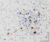 |
Fig. A.1. Finding chart of NGC 6649 from a 9′ × 9′ POSS2 Red image. Stars observed spectroscopically are marked with diferent colours according to their spectral types. The identification of each star corresponds to the WEBDA numbering for this cluster. North is up and east is left. |
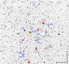 |
Fig. A.2. Finding chart of NGC 6664 from a 19′ × 17′ POSS2 Red image. Stars observed spectroscopically are marked with diferent colours according to their spectral types. The identification of each star corresponds to the WEBDA numbering for this cluster. North is up and east is left. |
 |
Fig. A.3. Finding chart of Be 55 from a 8′ × 8′ POSS2 Red image. Stars observed spectroscopically are marked with diferent colours according to their spectral types. The identification of each star follows the numbering given by Negueruela & Marco (2012). North is up and east is left. |
All Tables
Equatorial coordinates (J2000) for the centre and core (rc) and tidal (rt) radii for the studied clusters.
Stellar atmospheric parameters for the cool stars derived from high-resolution spectra.
Chemical abundances, relative to solar abundances by Grevesse et al. (2007), measured on the cool stars in the field of NGC 6649.
Chemical abundances, relative to solar abundances by Grevesse et al. (2007), measured on the cool stars in the field of NGC 6664.
Comparison of the cluster sizes (arcmin) derived in this work and in the literature.
Comparison of the results obtained for the Cepheid V367 Sct from this work (TW) and Genovali et al. (2014) for the stellar atmospheric parameters and Genovali et al. (2015) for the chemical abundances, relative to solar values from Grevesse et al. (2007).
Age (Ma) and mass (M⊙) of cluster Cepheids derived from their parent cluster (inferred from isochrones) and by using different period-age (PAR) and mass-luminosity (MLR) relations.
Number of red (super)giant stars and yellow supergiants, (Cepheids or not, in brackets) in open clusters with ages between 50 and 150 Ma (from Mermilliod et al. 2008).
Gaia DR2 astrometric data and cluster membership for all stars observed spectroscopically in this work.
All Figures
|
Fig. 1. Spectra of the cool stars observed in the field of NGC 6649. With the only exception of S19, observed with ISIS, these stars were observed with FEROS (we note the gap between orders 37 and 38 around 8540 Å). |
| In the text | |
|
Fig. 2. HERMES spectra for cool stars in the field of NGC 6664 (we note the gap between orders 41 and 42 around 8580 Å). |
| In the text | |
|
Fig. 3. V/(B − V) diagram for all stars in the field of NGC 6649. Stars with only BV photometry are represented by gray dots whereas those observed also in the U band appear as green dots. Stars for which we additionally have spectra are plotted with small blue circles (B-type stars), magenta diamond (Be star), and big circles: greenish-yellow for YSGs and red for RSGs. The numbering for the most representative stars is marked as well. |
| In the text | |
|
Fig. 4. Colour-magnitude diagrams for likely members of NGC 6649 in three different photometric systems: Left: MV/(B − V)0 from the optical photometry taken by Walker & Laney (1987); centre: MKS/(J − KS)0 (2MASS photometry); and right: G/(GBP − GRP) (Gaia DR2 data). Grey dots are the photometric data for likely members. Stars observed spectroscopically are represented as red circles (RSGs), greenish-yellow circles (YSGs), blue circles (blue stars), and magenta diamonds (Be stars). The black line shows the best-fitting PARSEC isochrone (log τ = 7.8). Star 2MASS J18335423-1019100, a possible new evolved member, is highlighted as a green triangle. |
| In the text | |
|
Fig. 5. Colour–magnitude diagrams for likely members of NGC 6664. Colours and symbols are the same as those in Fig. 4. The black line shows the best-fitting PARSEC isochrone (log τ = 7.90). Star BD-08 4641, a good candidate to be a new YSG cluster member, is highlighted as a brown square that is very close to the Cepheid EV Sct. |
| In the text | |
|
Fig. 6. Colour-magnitude diagrams for likely members of Be 55. Colours and symbols are the same as those in Fig. 4. The solid line shows the best-fitting PARSEC isochrone (at the Cepheid metallicity) whereas the dashed line corresponds to that computed at [Fe/H] = −0.4 (see text for details). |
| In the text | |
|
Fig. 7. Projected density distribution around the clusters studied in this work. Red circles are the observed values together with the Poisson errors whereas the blue line shows the fitted King profile. Vertical dashed lines represents the core (rc) and tidal (rt) radii while the horizontal one is the background density. |
| In the text | |
|
Fig. 8. Kiel diagram for likely members in NGC 6649 and NGC 6664. Colours and symbols are the same as those in Fig. 4. |
| In the text | |
|
Fig. 9. Iron abundance gradient in the Milky Way found by Genovali et al. (2013, 2014). The black line is the Galactic gradient, green crosses are Cepheids studied in those papers, whereas black dots show data for other Cepheids from literature used by these authors. Magenta triangles represent young open clusters in the sample compiled by Netopil et al. (2016). The orange circle is NGC 6649 and the red one is NGC 6664. Finally, other clusters analysed by our group with the same technique are marked with star symbols. All the values shown in this plot are rescaled to Genovali et al. (2014), i.e., R⊙ = 7.95 kpc and A(Fe) = 7.50. |
| In the text | |
|
Fig. 10. Abundance ratios [X/Fe] versus [Fe/H]. The grey dots represent the Galactic trends for the thin disc (Adibekyan et al. 2012; Delgado Mena et al. 2017). NGC 6067, NGC 3105 and NGC 2345 are drawn with triangles (green, cyan, and blue, respectively), whereas NGC 6649 and NGC 6664 are the orange and red circles, respectively. Clusters are represented by their mean values. The dashed lines indicate the solar value. |
| In the text | |
|
Fig. A.1. Finding chart of NGC 6649 from a 9′ × 9′ POSS2 Red image. Stars observed spectroscopically are marked with diferent colours according to their spectral types. The identification of each star corresponds to the WEBDA numbering for this cluster. North is up and east is left. |
| In the text | |
|
Fig. A.2. Finding chart of NGC 6664 from a 19′ × 17′ POSS2 Red image. Stars observed spectroscopically are marked with diferent colours according to their spectral types. The identification of each star corresponds to the WEBDA numbering for this cluster. North is up and east is left. |
| In the text | |
|
Fig. A.3. Finding chart of Be 55 from a 8′ × 8′ POSS2 Red image. Stars observed spectroscopically are marked with diferent colours according to their spectral types. The identification of each star follows the numbering given by Negueruela & Marco (2012). North is up and east is left. |
| In the text | |
Current usage metrics show cumulative count of Article Views (full-text article views including HTML views, PDF and ePub downloads, according to the available data) and Abstracts Views on Vision4Press platform.
Data correspond to usage on the plateform after 2015. The current usage metrics is available 48-96 hours after online publication and is updated daily on week days.
Initial download of the metrics may take a while.