| Issue |
A&A
Volume 646, February 2021
|
|
|---|---|---|
| Article Number | A69 | |
| Number of page(s) | 15 | |
| Section | Cosmology (including clusters of galaxies) | |
| DOI | https://doi.org/10.1051/0004-6361/202037629 | |
| Published online | 09 February 2021 | |
Constraints on the spectral index of polarized synchrotron emission from WMAP and Faraday-corrected S-PASS data
1
Institute of Theoretical Astrophysics, University of Oslo, Blindern, Oslo, Norway
e-mail: unnif@astro.uio.no
2
Center for Computational Astrophysics, Flatiron Institute, 162 5th Avenue, New York, NY 10010, USA
Received:
31
January
2020
Accepted:
7
December
2020
We constrain the spectral index of polarized synchrotron emission, βs, by correlating the recently released 2.3 GHz S-Band Polarization All Sky Survey (S-PASS) data with the 23 GHz 9-year Wilkinson Microwave Anisotropy Probe (WMAP) sky maps. We subdivide the S-PASS field, which covers the southern ecliptic hemisphere, into 95 15° ×15° regions and estimate the spectral index of polarized synchrotron emission within each region using a simple but robust T–T plot technique. Three different versions of the S-PASS data are considered, corresponding to: no correction for Faraday rotation; Faraday correction based on the rotation measure model presented by the S-PASS team; or Faraday correction based on a rotation measure model presented by Hutschenreuter and Enßlin. We find that the correlation between S-PASS and WMAP is strongest when applying the S-PASS model. Adopting this correction model, we find that the mean spectral index of polarized synchrotron emission gradually steepens from βs ≈ −2.8 at low Galactic latitudes to βs ≈ −3.3 at high Galactic latitudes, in good agreement with previously published results. The flat spectral index at the low Galactic latitudes is likely partly due to depolarization effects. Finally, we consider two special cases defined by the BICEP2 and SPIDER fields and obtain mean estimates of βBICEP2 = −3.22 ± 0.06 and βSPIDER = −3.21 ± 0.03, respectively. Adopting the bandpass filtered WMAP 23 GHz sky map to only include angular scales between 2° and 10° as a spatial template, we constrain the root-mean-square synchrotron polarization amplitude to be less than 0.03 μK (0.009 μK) at 90 GHz (150 GHz) for the BICEP2 field, corresponding roughly to a tensor-to-scalar ratio of r ≲ 0.02 (r ≲ 0.005). Very similar constraints are obtained for the SPIDER field. A comparison with a similar analysis performed in the 23–33 GHz range suggests a flattening of about Δβs ∼ 0.1 ± 0.2 from low to higher frequencies, but with no statistical significance due to high uncertainties.
Key words: ISM: general / cosmology: observations / cosmic background radiation / diffuse radiation / Galaxy: general / polarization
© ESO 2021
1. Introduction
The field of observational cosmology has undergone a dramatic transformation in recent decades. The main driving force behind these developments has been rapidly improving instrumentation across the electromagnetic spectrum. This holds particularly true for measurements in the microwave range, which are essential for mapping the cosmic microwave background (CMB), an afterglow from the Big Bang. Such observations constrain cosmological parameters and models to sub-percent accuracy, the most prominent demonstration of which has been the European Space Agency’s (ESA) Planck satellite mission (Planck Collaboration I 2020; Planck Collaboration VI 2020).
While detailed measurements of the CMB temperature and polarization fluctuations have already transformed cosmology, such measurements further hold the promise of providing a unique window into the physics during the first tiny fraction of a second following the Big Bang. Specifically, according to the current standard cosmological concordance model, a quantum mechanical process called inflation (see, e.g., Liddle 1999, and references therein) took place shortly after the Big Bang, during which the effective length scale of the universe increased by a factor of 1028 or more during some 10−34 seconds. As a result of this process, space was violently stretched, and a background of so-called primordial gravitational waves was excited. These gravitational waves later warped spacetime during the epoch of recombination, stretching space in one direction and compressing it in the orthogonal direction, and created a particular unique signal in the CMB field that today can be observed in the form of so-called B-mode polarization (e.g., Zaldarriaga & Seljak 1997).
Robustly detecting the polarization signature of these primordial B-modes would provide cosmologists with a unique opportunity to constrain physics at the Planck scale. Unfortunately, the expected amplitude of the signal is very small for currently viable theories, ranging up to no more than 100 nK on large angular scales, and probably significantly less (BICEP2 Collaboration 2018). A wide range of these models are within reach, and even if these amplitudes are within the capabilities of modern detectors in terms of raw noise performance, another issue complicates the picture considerably, namely foreground emission from interstellar particles situated within the Milky Way. In particular, relativistic electrons moving within the Galactic magnetic field emit polarized synchrotron emission, whereas small vibrating dust grains aligned by the same magnetic field emit polarized thermal emission. Both of these foreground signals are very likely orders of magnitude brighter than the primordial gravitational wave signal on large angular scales (Planck Collaboration IV 2020).
Robustly distinguishing between the primordial and the local polarization signals is among the key challenges of modern CMB cosmology, and great efforts are being made to both establish observational constraints on the various effects and develop efficient computational and statistical methods to analyze the resulting data (e.g., Leach et al. 2008, and references therein). So far, stronger constraints have been derived for polarized thermal dust than for synchrotron, largely because the detectors needed to probe the relevant frequency range are smaller, cheaper, and more sensitive than the corresponding detectors required to probe synchrotron. Among the best examples of this are the Planck 217- and 353-GHz channels, which have revolutionized our understanding of polarized thermal dust in the CMB frequency range (Planck Collaboration XIX 2015).
Until very recently, the Wilkinson Microwave Anisotropy Probe (WMAP; Bennett et al. 2013) 23 GHz and Planck 30 GHz (Planck Collaboration II 2020) frequency channels provided the strongest constraints on polarized synchrotron emission. Subsequently, in March 2019 the first sky maps from the S-Band Polarization All Sky Survey (S-PASS; Carretti et al. 2019) were publicly released, observed at 2.3 GHz. Due to the spectral energy density power law relation of synchrotron emission, the signal at 2.3 GHz is in fact about 1000 times stronger than at 23 GHz, thus S-PASS provides a clear image of synchrotron emission in both intensity and polarization. The S-PASS map covers most of the southern celestial sphere (Dec < − 1°), for a total sky fraction of 48.7%. A total of 98.6% of all pixels have a reported polarization signal-to-noise higher than three. This makes S-PASS an excellent complement to WMAP and Planck, and jointly they should provide strong constraints on polarized synchrotron emission in the microwave regime. Indeed, an early analysis of this type has already been presented by Krachmalnicoff et al. (2018).
However, while the S-PASS data contain a wealth of information on synchrotron emission, their utility is significantly complicated by Faraday rotation (e.g., Beck et al. 2013). First discovered by Michael Faraday in 1845, this effect causes the rotation of the plane of polarization of an electromagnetic wave in the presence of a magnetic field. The effect is proportional to the strength of the magnetic field and the integrated electron density, as well as to the square of the wavelength of the wave. In an astrophysical setting, the Faraday rotation effect is therefore stronger for low frequencies and at low Galactic latitudes. For instance, while the magnitude of the effect is typically a few degrees at 23 GHz, it can be many hundreds of degrees at 2.3 GHz along the Galactic plane. Even at high Galactic latitudes, it can be several tens of degrees at this low frequency.
The magnitude of the Faraday rotation effect is typically quantified in terms of the rotation measure (RM), which is simply the proportionality constant that scales the square of the wavelength. Several models1 have been derived for the rotation measure, and in this paper we will consider and quantitatively compare three different models. The first is simply assuming no Faraday rotation at all, namely RM = 0. This serves as a baseline that allows us to assess the impact of the Faraday rotation effect. Our second model is that derived by the S-PASS team as part of the data release (Carretti et al. 2019). This model was derived as a joint fit to the S-PASS, WMAP 23 GHz, and Planck 30 GHz data sets. Our third and final model is that derived by Hutschenreuter & Enßlin (2020) through a Bayesian analysis of extra-galactic point sources and the Planck free-free map.
Throughout this paper we use a convention for polarization angles (PAs) where PA is 0° for vectors pointing north and increases westward. The same convention is used in experiments such as WMAP and Planck and differs from the International Astronomical Union (IAU) convention used in the S-PASS experiment where the PA increases eastward.
The rest of the paper is organized as follows. In Sect. 2 we briefly describe the data used in this paper, and in Sect. 3 we provide details on the Faraday rotation models we employ. The algorithms used to estimate the spectral index are described in Sect. 4, while the main results are presented in Sect. 4.2. In Sect. 4.3 we consider two special cases, namely the BICEP2 and SPIDER fields, both of which are covered by S-PASS. Finally, we conclude in Sect. 5.
2. S-PASS and WMAP data
The main goal of this paper is to estimate the synchrotron spectral index exploiting the statistical power of the recently released S-PASS sky map. To complement this map, we choose the WMAP 23 GHz sky map (Bennett et al. 2013), simply because it has higher signal-to-noise to polarized synchrotron emission compared to other available alternatives, most notably the Planck 30 GHz channel (Planck Collaboration I 2020).
First, we note that the S-PASS data were collected with the Parkes radio telescope, and therefore covers the southern celestial sky at Dec < − 1°, whereas the WMAP data are all-sky. As such, we apply an analysis mask, and consider only pixels within the S-PASS coverage, for a total of 48.7% of the sky.
Second, the S-PASS sky map has a native angular resolution of 8.9′ full width at half maximum (FWHM), whereas the WMAP 23 GHz sky map has a resolution of 53′ FWHM. Further, the two maps are pixelized on different grids, as S-PASS is defined on a HEALPix2 (Górski et al. 2005) grid with Nside = 1024 (3.4′ pixel size), while WMAP is defined on an Nside = 512 (6.7′ pixel size) grid. Our analysis requires both maps to be smoothed to a common angular resolution and pixelized with the same grid, and we therefore adopt a common resolution of 1° FWHM and Nside = 64 (55′ pixel size). Such a coarse pixel size ensures that neighboring pixels are only weakly correlated, and since no subsequent spherical harmonics transforms are involved in the analysis, operating with non-bandwidth limited maps, (i.e., corresponding to non-Nyquist sampling limited maps in the flat space case), is not a concern for this particular analysis.
For S-PASS we adopted an effective frequency of 2.303 GHz (Carretti et al. 2019), while for the WMAP 23 GHz sky maps we adopted an effective frequency of 22.45 GHz, corresponding to the effective frequency of a synchrotron spectrum scaling as ν−3 integrated over the WMAP bandpass (Page et al. 2003). At the low frequencies discussed in this paper, other sources of polarized emission (thermal dust being the dominant one) have a signal of about one percent of that of the synchrotron emission at a frequency of 23 GHz, while at the S-PASS frequency they are totally negligible. We therefore assume that both maps contain only polarized synchrotron emission and noise.
The top row of Fig. 1 shows the WMAP sky map in the S-PASS field, smoothed to 1° FWHM, while the second row shows the corresponding S-PASS sky map. Left and right columns show the Stokes Q and U parameters. As already noted in the introduction, we adopt the same convention for the polarization angles as WMAP and Planck. This is different from the S-PASS convention, for which the polarization angle increases eastward. To account for this difference, we multiply the S-PASS Stokes U parameter by −1.
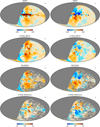 |
Fig. 1. Comparison of the main sky maps used in this analysis. From top to bottom, rows show the 23 GHz WMAP map (top row); the raw 2.3 GHz S-PASS (second row); the same S-PASS sky map, but corrected for Faraday rotation using the RM-SPASS (Carretti et al. 2019) model (third row); and the difference between the raw and the corrected S-PASS maps (bottom row). Left and right columns: Stokes Q and U components, respectively. All maps are smoothed to a common angular resolution of 1° FWHM, and all maps are plotted in brightness (Rayleigh-Jeans) temperature units. |
By eye, one can clearly see a strong correlation between the S-PASS and WMAP sky maps at high Galactic latitudes. However, at low latitudes there are major differences. Most notably, while WMAP exhibits a strong Q component, indicating a structured magnetic field oriented parallel to the Galactic plane, the S-PASS map has virtually no signal in the Galactic plane. This is a typical signature of Faraday rotation, which effectively rotates the polarization angle for a given emission source through a random angle before arriving at our location in the Milky Way. When integrating over many such sources, each with a random angle depending on its distance, the net sum is dramatically decreased. This is often referred to as “Faraday depolarization,” and is likely to flatten the spectral index in proximity to the Galactic plane.
3. Faraday rotation models and corrections
The total polarization angle ϕλ of linearly polarized light due to Faraday rotation, ϕRM, can be written as (e.g., Beck et al. 2013)
where ϕ0 is the intrinsic polarization angle of the source, RM is the rotation measure in units of rad m−2, and λ is the wavelength of the radiation. We consider two nontrivial models for the rotation measure in this paper constrained by direct measurements. The first model was presented as part of the S-PASS data release, and was derived through a joint fit to the S-PASS, WMAP, and Planck data (Carretti et al. 2019). The second model was presented by Hutschenreuter & Enßlin (2020), which used a combination of extra-galactic point sources and the Planck Commander free-free map to constrain the Galactic rotation measure within a Bayesian framework. Since this is measured using extra-galactic sources, it might not be an appropriate choice to correct the polarization angles of the diffuse emission considered in this paper. Nevertheless, we have chosen to include this template in the analysis. For completeness, we also consider the trivial case in which no correction for Faraday rotation is applied, namely RM = 0. We will refer to these three models as RM-SPASS, RM-HE, and RM-0, respectively.
Figure 2 compares RM-SPASS (top panel) and RM-HE (middle panel) in terms of the predicted rotation angle at 2.3 GHz. The bottom panel shows the difference between the two models. For both models we see that the predicted rotation angle is quite large for low Galactic latitudes, and small relative errors can therefore give large biases in a map that is rotated using these templates. It is also worth noting that the difference between the two models is substantial not only at low Galactic latitudes, but also at intermediate and high latitudes, at the level of tens of degrees.
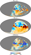 |
Fig. 2. Predicted Faraday rotation angle, ϕRM, at 2.3 GHz for the two models considered in this paper. Top panel: RM-SPASS model (Carretti et al. 2019), while middle panel: RM-HE model (Hutschenreuter & Enßlin 2020). Bottom panel: difference between the two models. All maps are shown in units of degrees. |
We note that the RM-SPASS model has many missing pixels within the S-PASS region. These are pixels for which the S-PASS collaboration considered the error on the RM or the difference in angle between WMAP and Planck angle maps too large to be reliable, and therefore did not provide an estimate. We also exclude these pixels in all subsequent analyses involving this model.
Considering that the center frequencies of the two data sets in question in this paper are 2.3 and 23 GHz, the predicted Faraday corrections for WMAP are roughly 100 times smaller than for S-PASS. As such, they only reach a few degrees in the central Galactic plane and are negligible at high latitudes. For this reason, we applied no corrections to WMAP.
Based on these models, we produced Faraday-corrected versions of the S-PASS sky map by performing the following rotation pixel-by-pixel,
Here (Q, U) denote the observed Stokes parameters, and (Q̂,Û) represent the Faraday-corrected Stokes parameters. The sign is chosen such that the correction corresponds to a negative rotation angle compared to those predicted by the model. This takes into account that the two RM models follow the IAU convention of the polarization angles.
If the adopted model represents an accurate estimate of the true sky, these Faraday corrections should improve the correlations between the S-PASS and WMAP data. We therefore compute the mean Pearson correlation coefficient between these two data sets for each of the three models as follows.
First, in order to trace spatial variations in both the synchrotron spectral index and the quality of the Faraday rotation model, we divide the full S-PASS sky field according to Nside = 4 regions, such that each region covers roughly 15° ×15° and contains 256 Nside = 64 pixels. Along the edge of the S-PASS survey, some of these regions are only partially filled, and we exclude any region for which more than half of the 256 pixels are excluded by the survey geometry. A total of 95 regions are retained by this criterion, as shown in Fig. 3. For the RM-SPASS maps, there are many missing pixels, and we have chosen to exclude regions where more than 75% of the pixels are missing, in this case ending up with 79 regions. Precise center locations for each region are listed in Table 1.
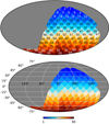 |
Fig. 3. Subdivision of the S-PASS region according to an Nside = 4 HEALPix grid. A total of 95 regions have more than 50% coverage within the S-PASS mask, and these form the primary basis for spatial localization in this paper. Top panel: region numbers, while bottom panel: a grid with galactic coordinates. The color range denote region number. |
Synchrotron spectral index for each region.
Second, for each region i, we compute the Pearson correlation coefficient between the Faraday-corrected S-PASS and the WMAP sky maps, minimized over local coordinate system orientations α,
where
is the Stokes Q parameter for pixel p measured in a coordinate system that is rotated by an angle α relative to the reference system, and is normalized by subtracting the average value. We note that α = 0° corresponds to the un-rotated Stokes Q parameter, while α = 45° corresponds to Stokes U. The motivation for performing this minimization procedure is simply to ensure that r is measured in the coordinate system with the lowest correlation (so that the reported r is a worst-case scenario). These correlation values should be interpreted with some caution. The numbers are not the true measure of the correlation in a region since we are only reporting the lowest value. We are only using them to compare the different data sets, and to exclude regions with obvious low correlation. We will also perform a similar coordinate system rotation when estimating the spectral index of polarized synchrotron emission, as was also done in Fuskeland et al. (2014).
Sky maps of r are plotted in Fig. 4 for each of the three models; RM-0 (top panel), RM-SPASS (middle panel), and RM-HE (bottom panel). The mean correlation coefficients averaged across the sky are r0 = 0.04 ± 0.3, rS − PASS = 0.46 ± 0.2, and rHE = 0.16 ± 0.3, respectively. Thus, while both RM-SPASS and RM-HE improves the overall correlation between S-PASS and WMAP, it is clear that the former yields an overall tighter agreement between the two data sets. This is of course not unexpected, considering the very different approaches taken by the two algorithms, in particular recognizing the fact that RM-SPASS exploits WMAP data directly, while RM-HE does not. Also, as mentioned previously, RM-HE is measured using extra-galactic point sources, and might not be very well suited for this analysis of diffuse emission.
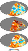 |
Fig. 4. Pearson correlation coefficient, r, evaluated between S-PASS data and WMAP data in regions spanning 15° ×15°. The WMAP data are the same in all panels, while the S-PASS data are, from top to bottom, (1) uncorrected data RM-0; (2) Faraday-corrected using RM-SPASS map (Carretti et al. 2019); and (3) Faraday-corrected using RM-HE (Hutschenreuter & Enßlin 2020). |
As a direct visualization of the corrections introduced by each of these models, Fig. 5 shows T–T scatter plots between the S-PASS and WMAP Stokes Q and U parameters for region 21. Clearly, the correlation is visually tighter for RM-SPASS than for either of the other two models, in agreement with the quantitative results reported above.
 |
Fig. 5. Comparison of T–T scatter plots for region 21 using different Faraday correction models. Both Stokes Q and U parameters are included in this figure, and the various symbols show (1) the uncorrected RM-0 data (black); (2) the Faraday-corrected data using RM-SPASS (Carretti et al. 2019) (red), and (3) the Faraday-corrected data using RM-HE Hutschenreuter & Enßlin (2020) (blue, crosses). The red dashed line is the best-fit slope using RM-SPASS. |
Returning for a moment to Fig. 1, the third row shows the S-PASS sky map after Faraday correction with the RM-SPASS model, while the bottom row shows the difference between the uncorrected and corrected S-PASS maps. Comparing the first and third rows, we see that the agreement with WMAP significantly improves after applying the Faraday correction. Furthermore, comparing the two bottom panels, we note that the magnitude of the Faraday correction ranges between a few percent to a factor of several tens. It is non-negligible in most areas on the sky, and is therefore essential to take into account in any joint analysis that combines S-PASS data with other observations. Based on these findings, we adopt the RM-SPASS model in the following.
4. Constraints on the spectral index of polarized synchrotron emission
4.1. Formalism
Our main goal in this paper is to use the S-PASS observations to constrain the spectral index of polarized synchrotron emission, βs. This parameter is defined by assuming that the effective spectral energy density of synchrotron emission follows a straight power law over the frequencies of interest. That is, we assume that the observed data, d, can be modeled as
where dν(p) denotes a vector of the Stokes Q and U parameters at frequency ν in pixel p; A is the amplitude of the signal at some reference frequency ν0; βi is the spectral index in region i; and nν denotes instrumental noise, which is typically assumed Gaussian with zero mean and known (co-)variance.
For such a simple model, one of the most robust standard methods for estimating βs is through so-called T–T plots. Fuskeland et al. (2014) applied this method to the WMAP 23 and 33 GHz data, instead of the WMAP 23 GHz and S-PASS 2.3 GHz data as we do here. We therefore refer the interested reader to that paper for full algorithmic details, and summarize only the main points here.
In the special case of noiseless data (n = 0), we see from Eq. (5) that the spectral index βs may be estimated from only two different data points through the following ratio,
Analogously, for noisy data one may fit a straight line, y = ax + b, to the distribution of pairs of observation, {dν1(p),dν2(p)}, and compute βs via the slope of the fitted line,
This is called the T–T plot technique, and it is a widely used tool in radio astronomy. The only slightly subtle point in this procedure is how to fit the straight line in the presence of noise in both data sets. However, several algorithms have been developed for precisely this purpose, and we adopt the effective variance method of Orear (1982), as implemented and described by Fuskeland et al. (2014).
To obtain robust results that are independent of the orientation of the (Galactic) coordinate system used to pixelize the S-PASS and WMAP data, we marginalize over polarization angle, similar to the procedure adopted for Faraday rotation assessment in the previous section. That is, we rotate the original data sets by an angle α into a new coordinate system by Eq. (4), considering all values of α between 0° and 85° in steps of 5°. We then estimate βs using the T–T plot approach for each value of α, and report either the full function βs(α) or the corresponding inverse-variance weighted mean
where σi is the uncertainty for a given value of α; see Eq. (14) in Fuskeland et al. (2014). These uncertainties are estimated by adding the statistical and systematic uncertainties in quadrature, and the systematic uncertainty is estimated using bootstrap sampling. That is, we randomly draw 10 000 new data combinations from the original data set, allowing duplicate points. Then the spectral indices are calculated for each new data set, and the standard deviation of this distribution is adopted as a systematic uncertainty.
4.2. Results
We now apply the method outlined above for each of the 95 regions defined in Fig. 3 to the Faraday-corrected S-PASS 2.3 GHz and the WMAP 23 GHz sky maps. Figure 6 shows individual T–T scatter plots for regions 1 through 48, for the Stokes Q and U parameters. The uncorrected and the RM-SPASS Faraday-corrected data are shown as black and red points, respectively. The best-fit straight lines when evaluating βi for all rotation angles α and taking the inverse-variance weighted means, are shown as their respective solid black and dashed red lines. Regions for which Pearson’s correlation coefficient is smaller than 0.2 are excluded from the analysis, and no best-fit lines are indicated in these cases. Also excluded are regions using the RM-SPASS data where more than 75% of the pixels are missing (Npix < 64). This results in a few regions where only the uncorrected data are used (regions 1, 2, 5, 58 and 86). Both of these types of excluded regions are flagged with a yellow background in Figs. 6–9.
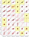 |
Fig. 6. T–T plots for Stokes Q and U for the uncorrected data (black, solid) and for the Faraday-corrected data using RM-SPASS (red, dashed). The lines are the fitted values of βtot. The yellow plots are where rSPASS < 0.2 or Npix < 64. Regions 1–48. |
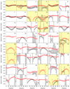 |
Fig. 7. Spectral index as a function of rotation angle for the uncorrected data (black, solid) and for the Faraday-corrected data (red, dashed). The lines are the values of βtot. The yellow plots are where rSPASS < 0.2, or Npix < 64. Regions 1–48. |
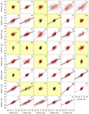 |
Fig. 8. T–T plots for Stokes Q and U for the uncorrected data (black, solid) and for the Faraday-corrected data using RM-SPASS (red, dashed). The lines are the fitted value of βtot. The yellow plots are where rSPASS < 0.2 or Npix < 64. Regions 49–95. |
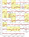 |
Fig. 9. Spectral index as a function of rotation angle for the uncorrected data (black, solid) and for the Faraday-corrected data (red, dashed). The lines are the values of βtot. The yellow plots are where rSPASS < 0.2 or Npix < 64. Regions 49–95. |
We observe large variations between the different regions in this figure. For instance, while regions 8 and 13 exhibit visually obvious correlations between S-PASS and WMAP, others, such as regions 12 and 48, require detailed statistical analysis to pick out a statistically significant correlation. Some regions show a large overall scatter, indicating that there are large signal variations inside these regions, while others show very small scatter and are dominated by instrumental noise.
Using the T–T plot method, we worked under the assumption that there is a common spectral index for all pairs of pixels within a region. However, this may not always be the case for our regions. So some of the scatter may be because of internal variation of the spectral index in a region.
Figure 7 shows the corresponding constraints on the spectral index βi as a function of rotation angle α for the same set of regions. Solid black points show results for uncorrected S-PASS data, while dashed red points show results for the RM-SPASS Faraday-corrected data. The horizontal lines indicate the respective inverse-variance weighted means.
Cases for which the black and red points agree closely primarily correspond to regions in which the magnitude and impact of the Faraday correction model is modest. This happens most typically at high Galactic latitudes, where the Galactic magnetic field is weak. The most typical case, however, is that the red points exhibit better coherence than the black points, suggesting that the Faraday correction is both significant and beneficial. Corresponding results for regions 49–95 are shown in Figs. 8 and 9.
Region 73 is an example of another interesting case. Here we observe large drifts as a function of rotation angle, but with very small uncertainty at each individual angle. Statistically speaking, there is a 3–4σ discrepancy between the spectral indices observed at α = 10° and 70°, with values ranging between −3.1 and −3.5. Taken at face value, this could in principle be interpreted as evidence for statistically significant variations in the spectral indices of the two Stokes parameters, Q and U, which is entirely possible from a physical point of view: Local alignment with the Galactic magnetic field or true spatial variations along each line-of-sight are only two physical effects that could create such a signal. However, very large variations are difficult to interpret in terms of physical variations in the local electron energy distribution. The applied RM maps may also rotate the low-frequency signal both in or out of phase with the high-frequency signal, resulting in either too shallow or too steep spectral index.
To account for further systematical uncertainties in the analysis, we conservatively adopted
as our final systematic estimate of the uncertainty on βs, evaluated separately for each region. This is added in quadrature to the uncertainty defined by the inverse-variance weighted average, which takes into account both the statistical uncertainty and the systematic uncertainty from the bootstrap procedure explained in Sect. 4.1. The statistical uncertainty gives a negligible contribution compared to the two systematical ones. All reported values are using the total uncertainty.
To test the impact of the errors that are distributed together with the RM maps from S-PASS, a full analysis have been made on S-PASS data that have been coherently rotated by ϕRM − SPASS + 1σRM − SPASS. This results in only a small shift of the regional spectral indices; maximum 1σ deviation in three regions and usually significantly less.
Final spectral index estimates for each region with correlation coefficients higher than 0.2, as defined by Eq. (3) and shown in Fig. 4, are listed in Table 1. Without Faraday correction, this includes 29 regions, while with RM-SPASS-based Faraday correction a total of 65 regions exceed the cut criterion. Figure 10 shows a histogram of these values.
 |
Fig. 10. Histogram of the polarized synchrotron spectral indices using the T–T plot method on S-PASS 2.3 GHz and WMAP 23 GHz data for the 19 accepted regions using uncorrected S-PASS data (black) and for the 65 accepted regions using Faraday-corrected S-PASS data (red). |
Inverse-variance weighting of the estimates for all regions yields a full-sky average of βs = −3.24 ± 0.01 with Faraday corrections and βs = −3.32 ± 0.02 without Faraday correction. The corresponding standard deviations are 0.09 and 0.19, respectively. These results are in excellent agreement with constraints derived from S-PASS and WMAP by Krachmalnicoff et al. (2018) using power spectra as their primary tool, reporting a full-sky average spectral index for polarized synchrotron emission of βs = −3.22 ± 0.08.
Figure 11 shows the spatial distribution of the mean spectral index of polarized synchrotron emission for each accepted region. Here we clearly see a statistically significant and systematic spatial variation in βtot, in the form of index steepening from low to high galactic latitudes. To quantify this observation further, we plot in Fig. 12 the average spectral index as a function of the absolute value of the Galactic latitude, |b|. Within each latitude bin, the various spectral indices have been inverse-variance weighted to produce a joint estimate, adopting the same methodology as described above for the full-sky average. Based on these measurements, we find that the spectral index typically range between βs = −2.7 and −2.9 along the Galactic plane, and between βs = −3.1 and −3.3 at high Galactic latitudes. The flat spectral index at low Galactic latitude are likely partly due to depolarization effects, which reduce the S-PASS amplitude and thus reduce the spectral index. This effect is only dominant in proximity of the Galactic plane, whereas for instance Krachmalnicoff et al. (2018) has chosen to exclude that region. Qualitatively speaking, this general behavior of the spectral index is in good agreement with the conclusions of numerous previous analyses, including Kogut et al. (2007), Fuskeland et al. (2014), Krachmalnicoff et al. (2018), all reporting significant steepening from low to high Galactic latitudes.
 |
Fig. 11. Spatial distribution of the polarized synchrotron spectral index between the Faraday-corrected S-PASS 2.3 GHz and WMAP 23 GHz data. Only regions for which the Pearson correlation coefficient r > 0.2 are shown. |
 |
Fig. 12. Polarized synchrotron spectral index as a function of the absolute value of latitude for the Faraday-corrected data (RM-SPASS). Regions at the same latitude are combined by estimating the inverse-variance weighted mean. Only regions for which the Pearson correlation coefficient is r > 0.2 are included. The horizontal line shows the inverse-variance weighted mean values of all regions, βtot = −3.24. |
4.3. Polarized synchrotron emission in the BICEP2 and SPIDER fields
Next, we consider two special cases of particular interest with respect to current and upcoming constraints on the tensor-to-scalar ratio, namely those corresponding to the BICEP2 (BICEP2 Collaboration 2018) and SPIDER (Nagy et al. 2017) fields. The BICEP2 field is defined approximately by a rectangle in celestial coordinates spanning −40° < RA < 40°, −65° < Dec < −50°, and covers about 1% of the sky. The central part of the SPIDER field is defined by 30° < RA < 70°, −55° < Dec < −15°, and covers about 8% of the sky. The two fields are analyzed in the same way as the previous regions, the number of pixels being 2305 (SPIDER) and 773 (BICEP2) in the uncorrected data, and reduced to 496 (SPIDER) and 486 (BICEP2) for the Faraday-corrected data due to the missing pixels.
The top panels of Fig. 13 show T–T plots between both the Faraday-corrected (red) and uncorrected (black) S-PASS and the WMAP data for each of these two fields. A strong correlation is observed in both cases. The bottom panels show corresponding βs(α) results for each field, and here we see that βs is well constrained for any value of α, suggesting that the final spectral index estimates are robust with respect to both instrumental effects and modeling errors. As reported in the bottom of Table 1, the mean spectral indices are βBICEP2 = −3.22 ± 0.06 and βSPIDER = −3.21 ± 0.03. For the BICEP2 field, the blue points show similar constraints derived from the WMAP 23 and 33 GHz data, as reported by Fuskeland et al. (2014); these are in good agreement with the new estimates, only with a lower signal-to-noise ratio. This previous analysis did not contain any analysis of the SPIDER field.
 |
Fig. 13. Results for the BICEP2 (left) and SPIDER (right) regions. The blue values are from Fig. 9 in Fuskeland et al. (2014) using the T–T plot method between the WMAP 23 GHz and 33 GHz data. |
These estimates may be used to predict the absolute level of polarized synchrotron emission at 90 and 150 GHz, the two primary CMB frequencies for both BICEP2 and SPIDER, by extrapolating the observed synchrotron amplitude at 23 GHz. To do this, we first computed two independent WMAP K-band “half-mission” maps by co-adding WMAP observation years 1–4 (HM1) and 5–9 (HM2). We smoothed each map to an effective angular resolution of 2° to suppress uncorrelated noise. Next, we formed an unbiased estimate of the square of the polarization amplitude per pixel by cross-correlating the two half-mission maps,
We note that because P̂2 is estimated as a cross-product between two half-mission maps, it can take on negative values. However, this can only happen due to P̂2 having anti-correlated noise fluctuations, and not true signal variations. We therefore estimate the linear polarization amplitude as
which is strictly positive. This quantity does not have a systematic noise bias due to auto-correlations, but only from the positivity prior, which is relevant only in low signal-to-noise regions.
The resulting WMAP 23 GHz P̂ map is shown in the top panel of Fig. 14, with the BICEP2 and SPIDER regions indicated by black lines. The bottom panel shows the same map, but after subtracting itself smoothed to 10° FWHM, thereby highlighting multipole moments between ℓ ≈ 20–100, or angular scales between 2° and 10°. The mean and standard deviation of the full map is 〈P̂〉 = 18 ± 6 μK within the BICEP2 region, and 7 ± 5 μK within the SPIDER region. Thus, the BICEP2 region has significantly higher polarized synchrotron emission levels than the SPIDER field, but most of this is only detectable on large angular scales. For the bandpass filtered map, both regions have a mean consistent with zero, while the standard deviations are 2.4 μK for the BICEP2 region, and 3.4 μK for the SPIDER region. These values largely reflects the instrumental noise level of the WMAP 23 GHz map, and they therefore only correspond to upper limits on the synchrotron level in these fields, not a determination of the actual synchrotron variation within each field.
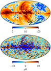 |
Fig. 14. WMAP K-band polarization amplitude, P̂, estimated by cross-correlating two half-mission maps. Top panel: smoothed to an effective angular resolution of 2° FWHM. Bottom panel: after bandpass filtering to include only scales between 2° and 10°, highlighting structures between ℓ ≈ 20 and 100. |
We can now estimate the polarization amplitude at 90 and 150 GHz by extrapolating P̂ from WMAP K-band (22.45 GHz), by scaling according to a power law model in brightness temperature, while properly accounting for unit conversions between brightness and thermodynamic units. The total extrapolation factor is given by
where g(ν)=(ex − 1)2/x2ex, x = hν/kTCMB is the conversion factor between brightness temperature and thermodynamic temperature units; h and k are the Planck and Boltzmann constants; and TCMB = 2.7255 K is the CMB temperature (Fixsen 2009).
Table 2 lists the extrapolated predictions for each region and multipole range, based on the mean spectral indices derived above. To set those values in context, we note that a tensor-to-scalar ratio of r = 0.1 induces a large-scale B-mode signal with standard deviation equal to 0.08 μK at a smoothing scale of 2° FWHM, while a ratio of r = 0.01 induces a B-mode standard deviation of 0.02 μK. After high-pass filtering, the polarized synchrotron contribution is therefore constrained to r ≲ 0.02 at 90 GHz and r ≲ 0.005 at 150 GHz for either field, within a small factor depending on the local noise properties of the WMAP survey.
Predictions for polarized synchrotron emission in the BICEP2 and SPIDER fields at a smoothing scale of 2° FWHM, based on WMAP 23 GHz and S-PASS.
4.4. Comparison with results in the 23–33 GHz range
Before concluding, we compare our results in the 2.3–23 GHz frequency range to similar results in the 23–33 GHz range, the latter obtained from Fuskeland et al. (2014) using WMAP K-band and WMAP Ka-band data. The analysis performed in Fuskeland et al. (2014) is similar to the one in this paper, but there are two main differences. The first one is that the 2014 analysis reports results as a straight mean derived by two methods, the T–T plot method, and a maximum likelihood method, while the current paper only applies the T–T plot method. For more details of the maximum likelihood method, see Fuskeland et al. (2014). The other difference is the region partitioning. Due to overall lower signal to noise ratio in the 2014 study, the full sky was divided into only 24 regions, where the diffuse regions were large and the regions inside a polarization foreground mask were smaller. A figure of the regions are shown in the top panel in Fig. 1 in Fuskeland et al. (2014).
For this comparison study we are only interested in pixels that are common in both papers. We use the final S-PASS pixels, and results, as shown in Fig. 11 minus a few particular bright objects, including the Galactic center, which were masked out in the 2014 analysis. There are large uncertainties in these two results, due to low signal to noise ratio in the 2014 data sets, and the results from the current paper are prone to Faraday rotation mis-modeling.
Figure 15 shows a 2D histogram of the values for the polarized synchrotron spectral indices from Fuskeland et al. (2014) versus the final, Faraday rotation corrected, results in this paper. The straight mean of the data points from the 2014 analysis, which is in the 23–33 GHz range, (y-axis) is −3.01 ± 0.14 while for the data points from this paper, in the 2.3–23 GHz range, (x-axis) is 3.15 ± 0.21. The bins are of size 0.1. Although the results are quite discrete because of the large regions in the 2014 paper, it shows that there is indeed a correlation between the results. The correlation line of y = x is shown on the figure. The figure suggests a flattening of about Δβs ∼ 0.1 ± 0.2 from low to higher frequencies. This is obtained by fitting a straight line with a slope equal to 1 to the data points in the figure. The uncertainty is reported as the standard deviation of the residuals in the fit. This flattening is interesting, but in no means conclusive due to large uncertainties associated with these results, so we find no statistical evidence for curvature between 2.3 and 33 GHz. A previous analysis (Kogut 2012) indicates a steepening toward higher frequencies, by an amount of Δβs = −0.07 for every octave in frequency. This analysis, however was done in intensity, and not polarization.
 |
Fig. 15. 2D histogram of the polarized synchrotron spectral indices from Fuskeland et al. (2014) (y-axis) versus the final results in this paper (x-axis). The set of pixels that are common to both studies are the final S-PASS pixels minus pixels around a few bright compact objects. The line y = x is shown. The figure indicates a flattening of about Δβs ∼ 0.1 from low to higher frequencies. The histogram column with the darkest blue color corresponds to about 1500 pixels of the total 10 830 pixels. |
5. Conclusions
In this paper we have constrained the spectral index of polarized synchrotron emission by correlating the recently released S-PASS 2.3 GHz data with the 9-year WMAP 23 GHz observations. This analysis has been performed using a simple but robust T–T technique, directly correlating the two maps in pixel space, and averaging over 15° ×15° regions. We find that the spectral index of polarized synchrotron emission steepens from βs ≈ −2.8 at low Galactic latitudes to βs ≈ −3.3 at high Galactic latitudes, in good agreement with several previous analyses. The flat spectral index at the lowest Galactic latitudes are likely to be partly due to the depolarization effect.
A similar study based on the same data combination has already been reported by Krachmalnicoff et al. (2018). The main fundamental difference between the two analyses lies in the different treatments of Faraday rotation. The former analysis was made by constraining the spectral index from the polarization amplitude that is not affected by Faraday rotation. In addition, they masked out regions for which the Faraday depolarization effect was considered dominant. In contrast, we actively correct the S-PASS observations before correlating the linear Stokes parameters with WMAP, and thereby avoid potential noise bias present in the polarization amplitude. Furthermore, we have considered two different models of the rotation measure for this purpose, namely the one presented by the S-PASS team derived directly from S-PASS, WMAP and Planck, and one produced by Hutschenreuter & Enßlin (2020) based on extra-galactic point sources and the Planck free-free map. While both models have an overall positive effect on the correlation between S-PASS and WMAP, the former results in a significantly higher correlation. This is expected, given its much closer connection with the data sets in question. Despite this important difference, we find that our results are in good qualitative agreement with those reported by Krachmalnicoff et al. (2018) at high Galactic latitudes.
These results are important for future constraints on the tensor-to-scalar ratio, as they provide insight on the overall level of spatial variations in the synchrotron spectral index. As an example, we applied our new constraints to estimate the level of synchrotron emission in the BICEP2 and SPIDER regions. Overall, we conclude the level of synchrotron emission on intermediate angular scales in these fields are constrained to r ≲ 0.02 at 90 GHz and r ≲ 0.005 at 150 GHz, where the upper limits are dominated by the noise properties of WMAP. Synchrotron emission is therefore unlikely to pose a serious challenge for the current generation of B-mode experiments. However, if all angular scales are considered, then the polarized synchrotron amplitude in the BICEP2 field corresponds to a tensor-to-scalar ratio of r ≳ 0.2. This difference between large and intermediate angular scales highlights the additional challenge required in order to detect the B-mode signal at very large angular scales, as is the target for future satellite missions such as LiteBIRD (Hazumi et al. 2019). Ultimately, ancillary information from ground-based low-frequency experiments such as S-PASS may play a very useful role in achieving this goal.
A comparison with results obtained from Fuskeland et al. (2014) has allowed us to investigate the polarized synchrotron spectral index in two different frequency ranges. This could indicate whether the power law relation we have used in this paper is a pure power law, as we have assumed, or if it should include curvature. Our analysis suggests a flattening of about Δβs ∼ 0.1 ± 0.2 from low to higher frequencies, in contrast to a previous analysis (Kogut 2012) that indicates a steepening. This is interesting, however in no means conclusive due to the large uncertainties associated with this analysis, so we find no statistical evidence for curvature between 2.3 and 33 GHz, but we cannot rule it out either. More analyses are needed and will show whether the synchrotron spectral index should be modeled with or without a curvature.
Acknowledgments
We acknowledge support from the European Union’s Horizon 2020 research and innovation program under grant agreement numbers 776282, 772253 and 819478, and from the Research Council of Norway. This work has made use of S-band Polarization All Sky Survey (S-PASS) data. Some of the results in this paper have been derived using the HEALPix (Górski et al. 2005) software and analysis package.
References
- Beck, R., Anderson, J., Heald, G., et al. 2013, Astron. Nachr., 334, 548 [NASA ADS] [CrossRef] [Google Scholar]
- Bennett, C. L., Larson, D., Weiland, J. L., et al. 2013, ApJS, 208, 20 [Google Scholar]
- BICEP2 Collaboration, Keck Array Collaboration (Ade, P. A. R., et al.) 2018, Phys. Rev. Lett., 121, 221301 [CrossRef] [PubMed] [Google Scholar]
- Carretti, E., Haverkorn, M., Staveley-Smith, L., et al. 2019, MNRAS, 489, 2330 [Google Scholar]
- Fixsen, D. J. 2009, ApJ, 707, 916 [Google Scholar]
- Fuskeland, U., Wehus, I. K., Eriksen, H. K., & Næss, S. K. 2014, ApJ, 790, 104 [NASA ADS] [CrossRef] [Google Scholar]
- Górski, K. M., Hivon, E., Banday, A. J., et al. 2005, ApJ, 622, 759 [NASA ADS] [CrossRef] [Google Scholar]
- Hazumi, M., Ade, P. A. R., Akiba, Y., et al. 2019, J. Low Temp. Phys., 194, 443 [Google Scholar]
- Hutschenreuter, S., & Enßlin, T. A. 2020, A&A, 633, A150 [EDP Sciences] [Google Scholar]
- Kogut, A. 2012, ApJ, 753, 110 [NASA ADS] [CrossRef] [Google Scholar]
- Kogut, A., Dunkley, J., Bennett, C. L., et al. 2007, ApJ, 665, 355 [NASA ADS] [CrossRef] [Google Scholar]
- Krachmalnicoff, N., Carretti, E., Baccigalupi, C., et al. 2018, A&A, 618, A166 [CrossRef] [EDP Sciences] [Google Scholar]
- Leach, S. M., Cardoso, J. F., Baccigalupi, C., et al. 2008, A&A, 491, 597 [NASA ADS] [CrossRef] [EDP Sciences] [Google Scholar]
- Liddle, A. R. 1999, in High Energy Physics and Cosmology, 1998 Summer School, eds. A. Masiero, G. Senjanovic, & A. Smirnov, 260 [Google Scholar]
- Nagy, J. M., Ade, P. A. R., Amiri, M., et al. 2017, ApJ, 844, 151 [NASA ADS] [CrossRef] [Google Scholar]
- Orear, J. 1982, Am. J. Phys., 50, 912 [Google Scholar]
- Page, L., Barnes, C., Hinshaw, G., et al. 2003, ApJS, 148, 39 [NASA ADS] [CrossRef] [Google Scholar]
- Planck Collaboration XIX. 2015, A&A, 576, A104 [NASA ADS] [CrossRef] [EDP Sciences] [Google Scholar]
- Planck Collaboration I. 2020, A&A, 641, A1 [CrossRef] [EDP Sciences] [Google Scholar]
- Planck Collaboration II. 2020, A&A, 641, A2 [CrossRef] [EDP Sciences] [Google Scholar]
- Planck Collaboration IV. 2020, A&A, 641, A4 [CrossRef] [EDP Sciences] [Google Scholar]
- Planck Collaboration VI. 2020, A&A, 641, A6 [NASA ADS] [CrossRef] [EDP Sciences] [Google Scholar]
- Zaldarriaga, M., & Seljak, U. 1997, Phys. Rev. D, 55, 1830 [Google Scholar]
All Tables
Predictions for polarized synchrotron emission in the BICEP2 and SPIDER fields at a smoothing scale of 2° FWHM, based on WMAP 23 GHz and S-PASS.
All Figures
 |
Fig. 1. Comparison of the main sky maps used in this analysis. From top to bottom, rows show the 23 GHz WMAP map (top row); the raw 2.3 GHz S-PASS (second row); the same S-PASS sky map, but corrected for Faraday rotation using the RM-SPASS (Carretti et al. 2019) model (third row); and the difference between the raw and the corrected S-PASS maps (bottom row). Left and right columns: Stokes Q and U components, respectively. All maps are smoothed to a common angular resolution of 1° FWHM, and all maps are plotted in brightness (Rayleigh-Jeans) temperature units. |
| In the text | |
 |
Fig. 2. Predicted Faraday rotation angle, ϕRM, at 2.3 GHz for the two models considered in this paper. Top panel: RM-SPASS model (Carretti et al. 2019), while middle panel: RM-HE model (Hutschenreuter & Enßlin 2020). Bottom panel: difference between the two models. All maps are shown in units of degrees. |
| In the text | |
 |
Fig. 3. Subdivision of the S-PASS region according to an Nside = 4 HEALPix grid. A total of 95 regions have more than 50% coverage within the S-PASS mask, and these form the primary basis for spatial localization in this paper. Top panel: region numbers, while bottom panel: a grid with galactic coordinates. The color range denote region number. |
| In the text | |
 |
Fig. 4. Pearson correlation coefficient, r, evaluated between S-PASS data and WMAP data in regions spanning 15° ×15°. The WMAP data are the same in all panels, while the S-PASS data are, from top to bottom, (1) uncorrected data RM-0; (2) Faraday-corrected using RM-SPASS map (Carretti et al. 2019); and (3) Faraday-corrected using RM-HE (Hutschenreuter & Enßlin 2020). |
| In the text | |
 |
Fig. 5. Comparison of T–T scatter plots for region 21 using different Faraday correction models. Both Stokes Q and U parameters are included in this figure, and the various symbols show (1) the uncorrected RM-0 data (black); (2) the Faraday-corrected data using RM-SPASS (Carretti et al. 2019) (red), and (3) the Faraday-corrected data using RM-HE Hutschenreuter & Enßlin (2020) (blue, crosses). The red dashed line is the best-fit slope using RM-SPASS. |
| In the text | |
 |
Fig. 6. T–T plots for Stokes Q and U for the uncorrected data (black, solid) and for the Faraday-corrected data using RM-SPASS (red, dashed). The lines are the fitted values of βtot. The yellow plots are where rSPASS < 0.2 or Npix < 64. Regions 1–48. |
| In the text | |
 |
Fig. 7. Spectral index as a function of rotation angle for the uncorrected data (black, solid) and for the Faraday-corrected data (red, dashed). The lines are the values of βtot. The yellow plots are where rSPASS < 0.2, or Npix < 64. Regions 1–48. |
| In the text | |
 |
Fig. 8. T–T plots for Stokes Q and U for the uncorrected data (black, solid) and for the Faraday-corrected data using RM-SPASS (red, dashed). The lines are the fitted value of βtot. The yellow plots are where rSPASS < 0.2 or Npix < 64. Regions 49–95. |
| In the text | |
 |
Fig. 9. Spectral index as a function of rotation angle for the uncorrected data (black, solid) and for the Faraday-corrected data (red, dashed). The lines are the values of βtot. The yellow plots are where rSPASS < 0.2 or Npix < 64. Regions 49–95. |
| In the text | |
 |
Fig. 10. Histogram of the polarized synchrotron spectral indices using the T–T plot method on S-PASS 2.3 GHz and WMAP 23 GHz data for the 19 accepted regions using uncorrected S-PASS data (black) and for the 65 accepted regions using Faraday-corrected S-PASS data (red). |
| In the text | |
 |
Fig. 11. Spatial distribution of the polarized synchrotron spectral index between the Faraday-corrected S-PASS 2.3 GHz and WMAP 23 GHz data. Only regions for which the Pearson correlation coefficient r > 0.2 are shown. |
| In the text | |
 |
Fig. 12. Polarized synchrotron spectral index as a function of the absolute value of latitude for the Faraday-corrected data (RM-SPASS). Regions at the same latitude are combined by estimating the inverse-variance weighted mean. Only regions for which the Pearson correlation coefficient is r > 0.2 are included. The horizontal line shows the inverse-variance weighted mean values of all regions, βtot = −3.24. |
| In the text | |
 |
Fig. 13. Results for the BICEP2 (left) and SPIDER (right) regions. The blue values are from Fig. 9 in Fuskeland et al. (2014) using the T–T plot method between the WMAP 23 GHz and 33 GHz data. |
| In the text | |
 |
Fig. 14. WMAP K-band polarization amplitude, P̂, estimated by cross-correlating two half-mission maps. Top panel: smoothed to an effective angular resolution of 2° FWHM. Bottom panel: after bandpass filtering to include only scales between 2° and 10°, highlighting structures between ℓ ≈ 20 and 100. |
| In the text | |
 |
Fig. 15. 2D histogram of the polarized synchrotron spectral indices from Fuskeland et al. (2014) (y-axis) versus the final results in this paper (x-axis). The set of pixels that are common to both studies are the final S-PASS pixels minus pixels around a few bright compact objects. The line y = x is shown. The figure indicates a flattening of about Δβs ∼ 0.1 from low to higher frequencies. The histogram column with the darkest blue color corresponds to about 1500 pixels of the total 10 830 pixels. |
| In the text | |
Current usage metrics show cumulative count of Article Views (full-text article views including HTML views, PDF and ePub downloads, according to the available data) and Abstracts Views on Vision4Press platform.
Data correspond to usage on the plateform after 2015. The current usage metrics is available 48-96 hours after online publication and is updated daily on week days.
Initial download of the metrics may take a while.


![$$ \begin{aligned} \left[ \begin{array}{c} \hat{Q} \\ \hat{U} \end{array}\right]=\left[ \begin{array}{cc} \cos 2\phi _{\mathrm{RM} }&\sin 2\phi _{\mathrm{RM} } \\ -\sin 2\phi _{\mathrm{RM} }&\cos 2\phi _{\mathrm{RM} } \end{array}\right]\left[ \begin{array}{c} Q \\ U \end{array}\right]. \end{aligned} $$](/articles/aa/full_html/2021/02/aa37629-20/aa37629-20-eq2.gif)


