| Issue |
A&A
Volume 633, January 2020
|
|
|---|---|---|
| Article Number | A16 | |
| Number of page(s) | 24 | |
| Section | Numerical methods and codes | |
| DOI | https://doi.org/10.1051/0004-6361/201936584 | |
| Published online | 23 December 2019 | |
A 3D short-characteristics method for continuum and line scattering problems in the winds of hot stars
1
LMU München, Universitätssternwarte, Scheinerstr. 1, 81679 München, Germany
e-mail: This email address is being protected from spambots. You need JavaScript enabled to view it.
, This email address is being protected from spambots. You need JavaScript enabled to view it.
2
Instituut voor Sterrenkunde, KU Leuven, Celestijnenlaan 200D, 3001 Leuven, Belgium
Received:
27
August
2019
Accepted:
8
October
2019
Abstract
Context. Knowledge about hot, massive stars is usually inferred from quantitative spectroscopy. To analyse non-spherical phenomena, the existing 1D codes must be extended to higher dimensions, and corresponding tools need to be developed.
Aims. We present a 3D radiative transfer code that is capable of calculating continuum and line scattering problems in the winds of hot stars. By considering spherically symmetric test models, we discuss potential error sources, and indicate advantages and disadvantages by comparing different solution methods. Further, we analyse the ultra-violet (UV) resonance line formation in the winds of rapidly rotating O stars.
Methods. We consider both a (simplified) continuum model including scattering and thermal sources, and a UV resonance line transition approximated by a two-level-atom. We applied the short-characteristics (SC) method, using linear or monotonic Bézier interpolations, for which monotonicity is of prime importance, to solve the equation of radiative transfer on a non-uniform Cartesian grid. To calculate scattering dominated problems, our solution method is supplemented by an accelerated Λ-iteration scheme using newly developed non-local operators.
Results. For the spherical test models, the mean relative error of the source function is on the 5 − 20% level, depending on the applied interpolation technique and the complexity of the considered model. All calculated line profiles are in excellent agreement with corresponding 1D solutions. Close to the stellar surface, the SC methods generally perform better than a 3D finite-volume-method; however, they display specific problems in searchlight-beam tests at larger distances from the star. The predicted line profiles from fast rotating stars show a distinct behaviour as a function of rotational speed and inclination. This behaviour is tightly coupled to the wind structure and the description of gravity darkening and stellar surface distortion.
Conclusions. Our SC methods are ready to be used for quantitative analyses of UV resonance line profiles. When calculating optically thick continua, both SC methods give reliable results, in contrast to the alternative finite-volume method.
Key words: radiative transfer / methods: numerical / stars: massive / stars: rotation / stars: winds / outflows
© ESO 2019
1. Introduction
Understanding of hot, massive stars is a basic prerequisite for interpreting fundamental properties of our Universe. Already during their lifetimes, such stars influence the evolution of galaxies via feedback of ionizing radiation and radiatively driven winds, and they enrich the interstellar medium (ISM) with metals. But also, their deaths are of large impact. Depending on initial mass and mass loss, OB stars either explode as supernovae or end up as “heavy” stellar-mass black holes (Heger et al. 2003). Obviously, supernova explosions enrich the ISM with metals even further. Additionally, the associated shock fronts possibly trigger star formation, resulting in a new generation of (massive) stars.
With the advent of gravitational wave (GW) observations (e.g. the black hole merger GW150914 observed at the advanced Laser Interferometric Gravitational-Wave Observatory (aLIGO), Abbott et al. 2016), the formation of heavy stellar-mass black holes becomes of key interest. Since massive stars are frequently found to be members of multiple star systems (see, e.g. Mason et al. 2009; Sana et al. 2013), they might explain the occurrence of GW events in the correct mass range. At least the formation of heavy black holes from single-star evolution, however, requires comparatively moderate mass loss rates (e.g. in low metalicity environments, or mass-loss quenching by magnetic fields, Petit et al. 2017; Keszthelyi et al. 2017).
Current knowledge of OB stars is inferred from quantitative spectroscopy, that is, by comparing observed spectra with synthetic ones, the latter being obtained from numerically modelling their stellar atmospheres (photosphere + wind). State of the art atmospheric modelling is performed by assuming spherical symmetry (e.g. CMFGEN: Hillier & Miller 1998; PHOENIX: Hauschildt 1992; POWR: Gräfener et al. 2002; WM-BASIC: Pauldrach et al. 2001; FASTWIND: Puls et al. 2005; Rivero González et al. 2012).
Several effects may alter the geometry of hot star atmospheres, affecting both the photospheric and wind lines. For instance, binary interaction (see, e.g. Vanbeveren 1991; de Mink et al. 2013 for a discussion about evolutionary aspects, and Prilutskii & Usov 1976; Cherepashchuk 1976; Stevens et al. 1992 for the effects of colliding winds) influences the line formation in such objects. Another example is the phenomenon of magnetic winds (e.g. ud-Doula & Owocki 2002; ud-Doula et al. 2008; Petit et al. 2013), for which the resonance line formation has been extensively discussed in Marcolino et al. (2013), Hennicker et al. (2018), and David-Uraz et al. (2019), for instance. Additionally, (non-radial) pulsations may impact the geometry of hot star atmospheres.
In this paper, we focus on (rapidly) rotating stars. In addition to polar velocity components that affect the radiative line-driving, such stars and their winds are influenced by centrifugal forces and gravity darkening. For a detailed discussion, we refer to Sect. 5.
To analyse these effects, and to distinguish between different theories (resulting in, e.g. prolate vs. oblate wind structures), multi-D radiative transfer codes that include a treatment of (arbitrary) velocity fields are required. In hot star winds, a key challenge is the implementation of scattering processes. Such problems are most easily handled by an accelerated Λ-iteration scheme, that is, by calculating the radiation field for known sources and sink terms (the so-called formal solution), and iterating the updated sources and sinks until convergence (Cannon 1973).
In order to obtain the formal solution in multi-D, the following two major methods exist, each having specific advantages and disadvantages. Firstly, within the finite-volume method (FVM, see Adam 1990 for the first application in the context of radiative transfer problems), the calculation volume is discretized into finite sub-volumes. All required physical values at the cell centres are then considered as suitable averages within each cell. This way, a relatively simple solution scheme can be derived, which, however, is only of low order. Thus, the FVM breaks down for large optical depths (Hennicker et al. 2018, hereafter Paper I). Nevertheless, it is still useful for qualitative interpretations (see, e.g. Lobel & Blomme 2008 for an application to corotating interaction regions in the winds of rotating stars). Secondly, within the characteristics methods, the formal solution is obtained by exact integration of the equation of radiative transfer along a ray. One distinguishes between the “long-characteristics” method (LC, Jones & Skumanich 1973; Jones 1973), and the “short-characteristics” method (SC, Kunasz & Auer 1988). The LC method follows a particular ray from the boundary to the considered grid point, whereas the SC method considers rays only from cell to cell. All required quantities at each upwind point are obtained from interpolation. While the LC method is computationally more expensive than the SC method, the latter introduces numerical errors from the interpolation scheme. To date, few 3D codes that apply one or the other technique already exist, such as PHOENIX/3D (Hauschildt & Baron 2006 and other publications in this series) and IRIS (Ibgui et al. 2013), which, however, are either proprietary, or do not include a suitable Λ-iteration scheme. For additional information on other codes, we refer to Sect. 1 of Paper I.
In this paper, we present a newly developed 3D SC code, which is capable of treating arbitrary velocity fields, and includes an accelerated Λ-iteration scheme to handle continuum and line scattering problems. In Sect. 2, we discuss the basic assumptions of the code. The numerical methods are described in Sect. 3. In Sect. 4, we perform a detailed error analysis by comparing our 3D results for spherically symmetric atmospheres with corresponding 1D solutions. Additionally, we present comparisons with the 3D finite-volume method from Paper I, when appropriate. As a first application to non-spherical winds, we calculated UV resonance line profiles for different models of rotating stars in Sect. 5, and discuss the implications. Our conclusions are summarized in Sect. 6.
2. Basic assumptions
In this paper, we use the same basic assumptions as in Paper I, that is we aim to solve the time-independent equation of radiative transfer (e.g. Mihalas 1978), formulated in the observer’s frame:
 (1)
(1)
Iν describes the specific intensity for a given frequency ν and direction n, and χν and Sν are the opacities (in units of cm−1) and source functions for continuum and line processes. For our following tests, we either consider a pure continuum case with source function
 (2)
(2)
and thermalization parameter ϵC, or a line (within an optically thin continuum) approximated by a two-level-atom (TLA). A generalization to a multitude of lines, coupled via corresponding rate equations, is one of our next objectives. Within the TLA approach, the line source function reads:
 (3)
(3)
![Mathematical equation: $$ \begin{aligned} \epsilon _{\rm L}&= \dfrac{\epsilon ^{\prime }}{1+\epsilon ^{\prime }} , \quad \epsilon ^{\prime }=\dfrac{C_{\rm ul}}{A_{\rm ul}}\Biggl [1-\exp \Bigl (-\frac{h \nu }{k_{\rm B} T} \Bigr ) \Biggr ]\cdot \end{aligned} $$](/articles/aa/full_html/2020/01/aa36584-19/aa36584-19-eq4.gif) (4)
(4)
 is the “scattering integral” (see Eq. (25)), and Cul and Aul describe the collisional rate and Einstein coefficient for spontaneous emission, respectively. In this paper, ϵL is considered as input parameter. The profile function Φx is approximated by a Doppler profile:
![Mathematical equation: $$ \begin{aligned} {\Phi _x}= \dfrac{1}{\sqrt{\pi }\delta } \exp \Biggl [-\Bigl (\dfrac{x_{\rm cmf}}{\delta } \Bigr )^2\Biggr ] = \dfrac{1}{\sqrt{\pi }\delta } \exp \Biggl [- \left(\dfrac{x_{\rm obs}- {\boldsymbol{n}} \cdot {\boldsymbol{V}}}{\delta } \right)^2\Biggr ] , \end{aligned} $$](/articles/aa/full_html/2020/01/aa36584-19/aa36584-19-eq6.gif) (5)
(5)
where xcmf and xobs denote the frequency shift from line centre in the comoving and observer’s frame, in units of a fiducial Doppler width,  . V is the local velocity vector in units of
  , and
, and
 (6)
(6)
is the ratio between the local thermal velocity (accounting for micro-turbulent velocities) and the fiducial thermal velocity. This description of the profile function allows for a depth-independent frequency grid (see also Paper I).
Finally, we express the continuum and line opacities in terms of the Thomson-opacity, χTh = neσe, and depth-independent input parameters, kC, kL:
 (7)
(7)
 (8)
(8)
where the line-strength kL is related to the frequency integrated opacity  (e.g. Paper I, Eqs. (10) and (12), and with
 ![Mathematical equation: $ [\bar{\chi}_{\mathrm{0}}] $](/articles/aa/full_html/2020/01/aa36584-19/aa36584-19-eq13.gif) = (cm s)−1). In the following, we present (efficient) numerical tools for solving the coupled Eqs. (1)–(3). Since a direct solution is computationally prohibitive for 3D atmospheres due to limited memory capacity, we apply an accelerated Λ-iteration (ALI) scheme that overcomes the convergence problems of the classical Λ-iteration for optically thick, scattering dominated atmospheres by using an appropriate approximate Λ-operator (ALO).
= (cm s)−1). In the following, we present (efficient) numerical tools for solving the coupled Eqs. (1)–(3). Since a direct solution is computationally prohibitive for 3D atmospheres due to limited memory capacity, we apply an accelerated Λ-iteration (ALI) scheme that overcomes the convergence problems of the classical Λ-iteration for optically thick, scattering dominated atmospheres by using an appropriate approximate Λ-operator (ALO).
3. Numerical methods
The most time-consuming part of the ALI scheme consists of calculating the formal solution. In Paper I, we have shown that a formal solution obtained using the FVM suffers from various numerical inaccuracies related to numerical diffusion and to the order of accuracy, the latter influencing the solution particularly in the optically thick regime. To avoid these errors, we implement an integral method along short characteristics. When compared with a long-characteristics solution scheme, the computation time becomes reduced by roughly a factor of N/2, with N the number of spatial grid points (per dimension), since the LC method integrates the equation of radiative transfer along the complete path from the boundary to a considered grid point. Thus, LC methods become feasible only on massively parallelized architectures.
We follow the same approach as in Paper I, and solve the equation of radiative transfer on a non-uniform, 3-dimensional Cartesian grid. In contrast to curvilinear coordinate systems, the direction vector n then becomes constant with respect to the spatial grid, thus avoiding the otherwise required angular interpolation of upwind intensities and a complicated bookkeeping of intensities (and corresponding integration weights) for different directions. Furthermore, the sweep through the spatial domain is considerably simplified, and can be performed grid point by grid point along the x, y, and z coordinates, since the intensities (required for the upwind interpolation) are always known on the previous grid layer. To enable a straightforward implementation of non-monotonic velocity fields, we use the observer’s frame formulation.
SC methods have been successfully implemented already for 3D non-LTE (NLTE) radiative transfer problems in cool stars (e.g. Vath 1994; Leenaarts & Carlsson 2009; Hayek et al. 2010; Holzreuter & Solanki 2012). These codes, however, are mostly designed for planar geometries, and only account for subsonic and slightly supersonic velocity fields. For scattering problems including highly supersonic velocity fields, there exist, to our knowledge, only the 2D codes by Dullemond & Turolla (2000; planar/spherical), van Noort et al. (2002; planar/spherical/cylindrical), Georgiev et al. (2006) and Zsargó et al. (2006; spherical). The only 3D SC code including arbitrary velocity fields, IRIS (Ibgui et al. 2013), has also been formulated for planar geometries, and lacks the implementation of a Λ-iteration scheme thus far. As has been shown in all these studies, the final performance of the SC method crucially depends on the choice of the applied interpolation schemes.
3.1. The discretized radiative transfer equation along a ray
The equation of radiative transfer along a given direction can be written as
 (9)
(9)
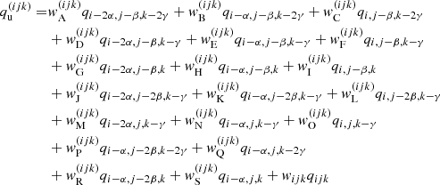
where dτ := χds is the optical-depth increment along a ray segment ds. Here and in the following, we suppress the notation for the frequency dependence, and explicitly distinguish between continuum and line only when appropriate. Equation (9) is integrated along a ray propagating through a current grid point p with Cartesian grid indices (ijk) and corresponding upwind point u(ijk). The geometry for a 3D Cartesian grid is shown in the upper panel of Fig. 1. In the following, upwind and downwind quantities corresponding to a considered grid point (ijk) are indicated by  and
and  , while local quantities are denoted either as
  or simply qijk. For a given ray segment, we then obtain:
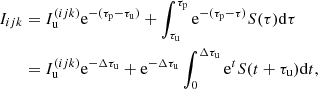 (10)
(10)
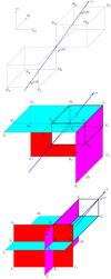 |
Fig. 1. Geometry of the SC method for a particular ray with direction n propagating from the upwind point u(ijk) to a considered grid point p(ijk). The downwind point d(ijk) is required to set the slope of a Bézier curve representing the opacities and source functions along the ray. The middle and lower panel display all possible downwind and upwind intersection surfaces for a short characteristic at a grid point p(ijk). For rays intersecting the xy-, xz-, and yz-planes, the 2D Bézier interpolation is obtained from given quantities at grid points located in the cyan, red, and magenta shaded surfaces, respectively. The coordinate system is indicated at the upper left, where α, β, γ determine the direction of the coordinate-axes and are defined in Sect. 3.3. |
with upwind optical-depth increment Δτu := τp − τu ≥ 0, and t := τ − τu. For the SC solution scheme, the location of the reference point, τ = 0, plays no role, since only the optical-depth increments, Δτu and Δτd (see below), are required. To calculate the source contribution, the source function is commonly approximated by first- or second-order polynomials (Kunasz & Auer 1988; van Noort et al. 2002), Bézier curves (Hayek et al. 2010; Holzreuter & Solanki 2012; Auer 2003) or cubic Hermite splines (Ibgui et al. 2013). While the 2nd- (and higher) order methods reproduce the diffusion limit in optically thick media, they suffer from overshoots and need to be monotonized with some effort to ensure that any interpolated quantity remains positive between two given grid points. Monotonicity is usually obtained by manipulating the interpolation scheme whenever overshoots occur. Thus, the actual interpolation crucially depends on the specific stratification of the considered quantity (e.g. the source function). The Λ-operator then becomes non-linear, because its elements now explicitly depend on the stratification of source functions (via corresponding interpolation/integration coefficients). Within any Λ-iteration scheme, this non-linearity can lead to oscillations. In extreme cases, “flip-flop situations” (Holzreuter & Solanki 2012, their Appendix A) may occur, which do not converge at all.
For the source contribution, we implement both a linear approximation as the fastest and most stable method (monotonicity is always provided), and a quadratic Bézier approximation (see Appendix B) for higher accuracy1, which allows us to preserve monotonicity in a rather simple way. The Bézier interpolation is constructed from two given data points and one control point, the latter setting the slope of the interpolating curve. The control point is located at the centre of the data-points abscissae, with the ordinate calculated by accounting for the information of a third data point to yield the parabola intersecting all three data points. Whenever overshoots occur, the value of the control point will be manipulated to ensure monotonicity (see Fig. B.2). The corresponding formulation is given in Appendix B, Eqs. (B.7)–(B.10). Applying these equations to describe the behaviour of the mean intensities along the optical path, and identifying the indices (i − 1), (i), (i + 1) with the upwind, current, and downwind points, we find, after reordering for the t0, t1, t2 terms:
![Mathematical equation: $$ \begin{aligned} \nonumber S(t+\tau _{\mathrm{u}}) =&S_{\mathrm{u}}^{({ijk})} + \Biggl [\dfrac{(\omega -2)}{\Delta \tau _{\mathrm{u}}}S_{\mathrm{u}}^{({ijk})} \\ \nonumber&+ \dfrac{(1-\omega )\Delta \tau _{\mathrm{u}}+(2-\omega )\Delta \tau _{\mathrm{d}}}{\Delta \tau _{\mathrm{u}}\Delta \tau _{\mathrm{d}}}S_{\mathrm{p}}^{({ijk})} + \dfrac{(\omega -1)}{\Delta \tau _{\mathrm{d}}}S_{\mathrm{d}}^{({ijk})} \Biggr ] \cdot t \\ \nonumber&+ \Biggl [ \dfrac{(1-\omega )}{\Delta \tau _{\mathrm{u}}^2}S_{\mathrm{u}}^{({ijk})} +\dfrac{(\omega -1)(\Delta \tau _{\mathrm{u}} + \Delta \tau _{\mathrm{d}})}{\Delta \tau _{\mathrm{u}}^2\Delta \tau _{\mathrm{d}}}S_{\mathrm{p}}^{({ijk})} \\&+\dfrac{(1-\omega )}{\Delta \tau _{\mathrm{u}}\Delta \tau _{\mathrm{d}}}S_{\mathrm{d}}^{({ijk})}\Biggr ] \cdot t^2 , \end{aligned} $$](/articles/aa/full_html/2020/01/aa36584-19/aa36584-19-eq19.gif) (11)
(11)
with downwind optical-depth increment, Δτd = τd − τp ≥ 0. The parameter ω defines the ordinate of the control point (Eq. (B.4)). Within the Bézier interpolation, we emphasize that ω may explicitly depend on  ,
,  , and
, and  to ensure monotonicity, and not solely on the grid spacing. A major advantage of this parameterization is that we can globally define a minimum allowed ω that can be adapted during the iteration process. The flip-flop situations discussed above can then be avoided by gradually increasing ωmin towards unity (ω ≡ 1 corresponds to a linear interpolation), that is, by suppressing the curvature of the Bézier interpolation. This way, we can construct an always-convergent iteration scheme, though with the drawback of using less accurate interpolations.
Integrating Eq. (10) together with a source function described by Eq. (11), we obtain the discretized equation of radiative transfer:
 (12)
(12)
with
The calculation of the upwind and downwind Δτ-steps proceeds similarly, where now the opacity is integrated using the Bézier interpolation. Using Eqs. (B.3), (B.4) for the upwind interval, and Eqs. (B.11), (B.12) for the downwind interval, one easily obtains:
![Mathematical equation: $$ \begin{aligned} \Delta \tau _{\mathrm{u}}&= \int _{\mathrm{u}}^{\mathrm{p}} \chi (s) \mathrm{d}s = \dfrac{\Delta s_{\mathrm{u}}}{3} (\chi _{\mathrm{u}} + \chi _{\mathrm{c}}^{[\mathrm{u},\mathrm{p}]} + \chi _{\mathrm{p}}) \end{aligned} $$](/articles/aa/full_html/2020/01/aa36584-19/aa36584-19-eq25.gif) (13)
(13)
![Mathematical equation: $$ \begin{aligned} \Delta \tau _{\mathrm{d}}&= \int _{\mathrm{p}}^{\mathrm{d}} \chi (s) \mathrm{d}s = \dfrac{\Delta s_{\mathrm{d}}}{3} (\chi _{\mathrm{p}} + \chi _{\mathrm{c}}^{[\mathrm{p},\mathrm{d}]} + \chi _{\mathrm{d}}), \end{aligned} $$](/articles/aa/full_html/2020/01/aa36584-19/aa36584-19-eq26.gif) (14)
(14)
where Δsu, Δsd describe the path lengths of the upwind and downwind intervals, respectively, and ![Mathematical equation: $ \chi_{{\text{ c}}}^{[{\text{ u}},{\text{ p}}]} $](/articles/aa/full_html/2020/01/aa36584-19/aa36584-19-eq27.gif) ,
, ![Mathematical equation: $ \chi_{{\text{ c}}}^{[{\text{ p}},{\text{ d}}]} $](/articles/aa/full_html/2020/01/aa36584-19/aa36584-19-eq28.gif) refer to the opacity at the control points in each interval.
refer to the opacity at the control points in each interval.
3.2. Grid refinement
Since the opacity of a line transition depends on the velocity field through the Doppler effect, regions of significant opacity may become spatially confined in a highly supersonic wind with strong acceleration. Thus, a grid refinement along the short characteristic might be required to correctly account for all so-called resonance zones. Because the profile function is approximated by a Doppler profile and rapidly vanishes for |xcmf/δ|≳3, a resonance zone is here defined by a region where xcmf/δ ∈ [ − 3, 3].
A numerically sufficient condition to resolve all such resonance zones along a given ray is to demand that |Δxcmf|/δ = |ΔVproj|/δ ≲ 1/3 if a resonance zone lies in between the points [u(ijk), p], where ΔVproj is the projected velocity step along the ray in units of  . Assuming a linear dependence of the projected velocities on the ray coordinate s, this condition directly translates to an equidistant refined spatial grid along the ray. For short ray segments (as is mostly the case within our calculations), neglecting the second-order (curvature) terms of the projected velocity influences the solution only weakly. The line source function on the refined grid is obtained by Bézier interpolation in s-space (Eqs. (B.7)–(B.9)):
 (15)
(15)
where the index ℓ refers to the points on the refined grid, and u(ijk), p(ijk), d(ijk) describe the original geometry of the short characteristic.  is obtained analogously, and the required Δτℓ steps are calculated with the trapezoidal rule, for simplicity. Contrasted to the Sobolev method (which also assumes a linear velocity law along the ray segment, e.g. Rybicki & Hummer 1978), our grid refinement procedure explicitly accounts for variations of the opacity and the source function.
Using Eq. (12) for the inter-grid points, such that the (local) upwind, current, and downwind quantities are now described by the indices [ℓ − 1, ℓ, ℓ + 1], we obtain:
 (16)
(16)
 (17)
(17)
 (18)
(18)
 (19)
(19)
For a number of Nref refinement points (including the upwind and current point) within the interval [u(ijk), p(ijk)], the intensity at point p(ijk) is finally given by:
 (20)
(20)
where the upwind and current points always correspond to the indices m = 1 and m = Nref, respectively, and the sum over m is performed over Nref − 1 intervals. The discretized radiative transfer equation for the refined grid obviously has the same form as for the standard short characteristic (Eq. (12)), with different coefficients though.
3.3. Upwind and downwind interpolations
To solve the discretized equation of radiative transfer, the opacities χC(u, d),  , source functions SC(u, d), SL(u, d), and velocity vectors V(u, d), are required at the upwind and downwind points, together with the incident intensity, Iu. We emphasize that the subscript C describes continuum quantities, and should not be confused with the subscript c denoting the control points of the interpolation scheme.
All required quantities are obtained from a 2D Bézier interpolation (see Appendix C) on the surfaces that intersect with a given ray. The intersection surfaces depend on the considered direction and the size of the upwind and downwind grid cells. For a given direction
 (21)
(21)
where θ is the co-latitude (measured from the Cartesian z-axis), and ϕ is the azimuth (measured from the x-axis), the distances from a considered grid point to the neighbouring xy-, xz-, and yz-planes are calculated from trigonometry and yield:
with α, β, γ set to ±1 for direction-vector components nx, ny, nz ≷ 0, respectively. The intersection surface on the upwind and downwind side are then found at the minimum of  , and the corresponding coordinates are easily calculated.
For each surface, the interpolation requires nine points within the corresponding plane (see Fig. 1 and Eq. (C.1)). In each considered plane, we generally use grid points running from (index-2) to (index) to determine upwind quantities, while downwind quantities are calculated from (index-1) to (index+1). Such a formulation greatly simplifies the calculation of the Λ-matrix elements (see Appendix D). In Fig. 1, we show an example for a ray intersecting the xy-plane at the upwind side. The 2D Bézier interpolation for the upwind point then consists of three 1D Bézier interpolations along the x-axis using the points (Ju, Ku, Lu), (Du, Eu, Fu), (Mu, Nu, Ou), followed by another 1D Bézier interpolation along the y-axis at the upwind x-coordinates. With the 2D Bézier interpolation given by Eq. (C.1), we find for each required quantity qu, d:
 (22)
(22)
 (23)
(23)
where the coefficients w(ijk) and  refer to the upwind and downwind interpolations corresponding to a considered point (ijk). Depending on the intersection surface, ten out of these 19 coefficients are set to zero. For the upwind interpolation, we have already included the local coefficient (ijk), which is only required when boundary conditions need to be specified (Sect. 3.4). We note that all (non-zero) interpolation coefficients may depend on the specific values of a considered quantity at the given grid points, via the interpolation parameter ω to ensure monotonicity. As in Sect. 3.1, also these monotonicity constraints result in non-linear Λ-operators.
3.4. Boundary conditions
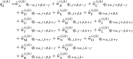
Since the inner boundary is usually not aligned with the 3D Cartesian grid (e.g. a spherical star at the origin), the upwind (and downwind) interpolations need to be adapted near the stellar surface. For the upwind point, the following two situations may occur (see Fig. 2 for an example in the xz-plane). Firstly, the considered ray originates from the stellar surface (direction n1 in Fig. 2). In this case, we use a core-halo approximation and set  , with
  the emergent intensity from the core, and Trad the radiation temperature. Unless explicitly noted, we assume Trad = Teff throughout this work. All other quantities are obtained from trilinear interpolation using the points (Eu, Fu, Hu, Iu, Nu, Ou, Su, p(ijk)) in Fig. 1, where representative estimates need to be defined at the core points (those points that are located inside the star). In hydrodynamic simulations, the analogue of these points are so-called “ghost points”. Secondly, the considered ray originates from a plane spanned by grid points that are partially located inside the star (direction n2 in Fig. 2). Then, the interpolation is performed as in Sect. 3.3, using again representative estimates at the core-points.
 |
Fig. 2. Boundary conditions for rays propagating in the xz-plane at y-level (j) with three different directions n1, n2, n3, and upwind points u1, u2, u3. For point u1, the intensity is set to |


Inside the core, we define  and set
  and all velocity components to zero, where
  is the inward directed intensity which needs to be specified only in rare situations (Fig. 2, direction n3). The opacities inside the star are found by extrapolation from the known values outside the star. While this procedure certainly introduces errors (e.g. by over- and underestimating the upwind source function in optically thin and thick cases, respectively), it is still favourable to extrapolating all values directly onto the stellar surface, mainly due to performance reasons2. In addition to the error introduced by the predefined values inside the core, the calculation of Δsr is a certain issue, where Δsr is the distance of the current grid point to the stellar surface. Since the radiative transfer near the stellar surface is (in most cases) very sensitive to the path length of a considered ray, Δsr needs to be known exactly. Depending on the shape of the surface, Δsr can be calculated analytically, or needs to be determined numerically. A numerical solution, however, might be time consuming and should be avoided when possible. Downwind quantities are always calculated from Eq. (23), using the estimates at the core points as defined above when necessary.
3.5. Angular and frequency integration
To obtain the mean intensity at each grid point in the atmosphere, we solve the discretized equation of radiative transfer for many directions and numerically integrate via:
 (24)
(24)
where wl is the integration weight corresponding to a considered direction Ωl = (θl, ϕl). The angular integration is particular challenging for optically thin atmospheres, since in such situations each (spatial) grid point is illuminated by the stellar surface, and the distribution of intensities Iijk(θ, ϕ) becomes a 2D step-function in the θ − ϕ-plane (if no upwind interpolation errors were present). Depending on the considered position, the shape of Iijk(θ, ϕ) greatly varies. Thus, elaborate integration methods are required to resolve the star and its edges at any point of the atmosphere.
Lobel & Blomme (2008) use the trapezoidal rule with a decreasing number of polar grid points at higher latitudes to reasonably distribute the direction vectors on the unit sphere. For the 3D FVM, we have shown in Paper I that a Gauss-Legendre integration performs (slightly) better. However, the corresponding directions are always clustered in certain regions since the nodes of the Gauss-Legendre quadrature are fixed. Additionally, the Gauss-Legendre integration should only be applied when the distribution of intensities can be described by high order polynomials, that is, when Iijk(θ, ϕ) is smoothed out (e.g. by numerical diffusion). When numerical diffusion errors are suppressed (e.g. by using elaborate upwind interpolation schemes), the Gauss-Legendre integration should not be used (see Table 1).
Mean relative error (defined in Sect. 4.2) of the mean intensity for a zero-opacity model, obtained using the Lebedev, Gauss-Legendre, and trapezoidal integration method, the latter with nodes from Lobel & Blomme (2008).
We have tested a multitude of other quadrature schemes, including trapezoidal and (pseudo)-Gaussian rules on triangles, and the so-called Lebedev quadrature (see, e.g. Ahrens & Beylkin 2009; Beentjes 2015, and references therein). The Lebedev quadrature is optimized to exactly integrate the spherical harmonics up to a certain degree, with a (nearly) optimum distribution of direction vectors on the unit sphere. In Table 1, we summarize the errors for an optically thin atmosphere using different integration methods. The incident intensities have been obtained exactly (i.e. by setting Iijk = Ic and Iijk = 0 for core and non-core rays, respectively), or from the 3D SC method using linear interpolations. Considering the SC solution scheme, the solution has only been slightly improved (if at all) when doubling the angular grid resolution from NΩ ≈ 1000 to NΩ ≈ 2000, for all applied integration methods. We note that the mean relative error does not converge to zero due to the upwind interpolation scheme (see Sect. 4.1). For the exact solution of the optically thin radiative transfer, the Lebedev-integration method performs best, and is therefore used within all our calculations. When calculating line transitions, the location of resonance zones depends on the considered direction. Thus, we generally use NΩ = 2030 direction vectors to ensure that no resonance zone has been overlooked. The corresponding angular resolution is typical when calculating 3D radiative transfer problems in extended stellar atmospheres. For instance, Lobel & Blomme (2008) used NΩ = 6400 within their 3D finite-volume method.
To obtain the scattering integral, we apply the trapezoidal rule for the frequency integration. The scattering integral then reads:
 (25)
(25)
with  and
and  the required frequency shift in the observer’s frame obtained from the maximum absolute velocity occurring in the atmosphere (see also Paper I), and wx the corresponding frequency integration weight. To resolve the profile function at each point in the atmosphere, we demand that |Δxobs|/δ ≲ 1/3. Since the profile function depends on the ratio of fiducial to actual thermal width, the fiducial velocity should be set to the minimum thermal velocity present in the atmosphere.
3.6. Λ-iteration
In Sect. 3.1, we have already noted that the Λ-operator becomes non-linear due to monotonicity constraints (implemented by the interpolation parameter ω). In this section, we present a suitable workaround, beginning with a recapitulation of some fundamental ideas.
3.6.1. Λ-matrix elements
With the discretized equation of radiative transfer, Eqs. (12)/(20), and the upwind and downwind quantities obtained from Eqs. (22) and (23), the intensity at each spatial, angular, and frequency grid point can be calculated for a given source function. We use the standard Λ-formalism to write the formal solution of the intensity, mean intensity, and scattering integral as:
![Mathematical equation: $$ \begin{aligned} I&= \Lambda _{\Omega ,\nu }[S_{\rm C, L}] \end{aligned} $$](/articles/aa/full_html/2020/01/aa36584-19/aa36584-19-eq59.gif) (26)
(26)
![Mathematical equation: $$ \begin{aligned} J&= \Lambda _{\nu }[S_{\rm C}] \end{aligned} $$](/articles/aa/full_html/2020/01/aa36584-19/aa36584-19-eq60.gif) (27)
(27)
![Mathematical equation: $$ \begin{aligned} \bar{J}&= \Lambda [S_{\rm L}], \end{aligned} $$](/articles/aa/full_html/2020/01/aa36584-19/aa36584-19-eq61.gif) (28)
(28)
with subscripts Ω and ν defining the dependence of the Λ-operator on direction and frequency, respectively. In the following, we focus on the line transport. The continuum can be derived analogously. When all interpolation parameters ω have been determined (for a given stratification of source functions and intensities), the Λ-operator is an affine operator described by the Λ-matrix and a constant displacement vector ΦB representing the propagation of boundary conditions (for a detailed discussion, see Paper I, Puls 1991, and references therein). The Λ-matrix elements can then be obtained by:
 (29)
(29)
with the nth unit vector en, and matrix indices m, n related to the 3D indices (i, j, k) by
 (30)
(30)
where Nx and Ny denote the number of spatial grid points of the x and y coordinate, respectively. Equation (30) simply transforms a data cube to a 1D array. The m, nth matrix-element describes the effect of a non-vanishing source function at grid point n onto grid point m. We emphasize that Eq. (29) holds only for pre-calculated interpolation parameters ω, obtained from an already known stratification of source functions.
3.6.2. Accelerated Λ-iteration
The classical Λ-iteration scheme is defined by calculating a formal solution for a given source function using Eq. (28), followed by the calculation of a new source function by means of Eq. (3). For optically thick, scattering dominated atmospheres, however, this iteration scheme suffers from severe convergence problems (see Fig. 5 for the convergence behaviour of spherically symmetric test models). To overcome these problems, we apply an accelerated Λ-iteration scheme based on operator-splitting methods (Cannon 1973). Within the ALI, the Λ-operator is written as
 (31)
(31)
where the first term is an appropriately chosen ALO acting on the new source function,  , and the second term acts on the previous one,
  . For the converged solution, this scheme becomes an exact relation. Using also, and in analogy to the exact Λ-operator, an affine representation for the approximate one, Λ(A)[S] = Λ* ⋅ S + ΦB (cf. above), and evaluating Λ(A) at the previous iteration step, k − 1, we obtain:
![Mathematical equation: $$ \begin{aligned} \nonumber {\boldsymbol{S}}^{(k)}_{\rm L}&= {\boldsymbol{\zeta }} \cdot \bar{{\boldsymbol{J}}}^{(k)} + {\boldsymbol{\Psi }} \\ \nonumber&\approx {\boldsymbol{\zeta }} \cdot \Lambda ^\mathrm{(A)}_{k-1}[{\boldsymbol{S}}_{\rm L}^{(k)}] + {\boldsymbol{\zeta }} \cdot (\Lambda _{k-1}-\Lambda ^\mathrm{(A)}_{k-1}) [{\boldsymbol{S}}_{\rm L}^{(k-1)}] + {\boldsymbol{\Psi }}\\ \nonumber&= {\boldsymbol{\zeta }} \cdot \Bigl ( {\boldsymbol{\Lambda }}^*_{k-1} {\boldsymbol{S}}_{\rm L}^{(k)} + {\boldsymbol{\Phi }}_{\rm B}^{(k-1)} + \bar{{\boldsymbol{J}}}^{(k-1)} - {\boldsymbol{\Lambda }}^*_{k-1} {\boldsymbol{S}}_{\rm L}^{(k-1)} - {\boldsymbol{\Phi }}_{\rm B}^{(k-1)} \Bigl )+ {\boldsymbol{\Psi }}. \\ \end{aligned} $$](/articles/aa/full_html/2020/01/aa36584-19/aa36584-19-eq67.gif) (32)
(32)
Here, the iteration indices k − 1 and k are indicated as sub- or superscripts, ζ := 1 − ϵL is a diagonal matrix, and Ψ := ϵL ⋅ Bν(T) is the thermal contribution vector. From Eq. (32), it is obvious that the ΦB terms cancel. For multi-level atoms, we emphasize that Λ and Λ(A) may change within the ALI-cycle due to the variation of opacities (induced by the subsequently updated occupation numbers). Furthermore, both operators might also change even for the simplified TLA approach considered in this paper, since the corresponding matrix elements depend on the source functions via the interpolation parameters ωk − 1, ωk. Rearranging terms, we find:
 (33)
(33)
Equation (33) is solved to obtain a new source function  (see below). Since, however,
  has been optimized only to ensure monotonicity in a specific step k − 1 (based on source function
  ), the iteration scheme can oscillate due to oscillations in
  and
and  . Even worse, the new source function might become negative. To overcome these problems, non-linear situations need to be avoided (by providing almost constant Λ*-matrices over subsequent iteration steps). The following approach has proved to lead to a stable and convergent scheme: We apply purely linear interpolations (ωk − 1 = ωk = 1 and thus
  ) in the first four iteration steps to obtain an already smooth stratification of source functions. Additionally, we globally define a minimum allowed interpolation parameter and demand that ω > ωmin. Then, ω becomes constant (namely ω = ωmin) in (most) critical situations, and again,
  approaches
  . Whenever negative source functions or oscillations occur within the iteration scheme, ωmin is gradually increased to one. With this approach, we obtain an always convergent iteration scheme, with a formal solution obtained by using linear interpolations only in most challenging cases.
3.6.3. Constructing the ALO
The rate of convergence achieved by the accelerated Λ-iteration scheme increases with the number of Λ-matrix elements included in the ALO. To minimize the computation time of the complete procedure, the choice of the ALO is always a compromise between the number of matrix-elements to be calculated, and the resulting convergence speed. While the inversion of a diagonal ALO reduces to a simple division, a multi-band ALO needs to be inverted with some more effort. When taking only the nearest neighbours into account, however, the ALO becomes a sparse matrix, and can be efficiently inverted by applying the Jacobi-Iteration for sparse systems (see Paper I). For 3D calculations, a multi-band ALO is required to obtain a rapidly converging iteration scheme (see Hauschildt & Baron 2006 and Paper I for solutions obtained with the LC method and the FVM, respectively), and thus implemented within our 3D SC framework. To calculate the corresponding Λ-matrix elements (including all upwind and downwind interpolations), we extend the procedure developed by Olson & Kunasz (1987) and Kunasz & Olson (1988). A detailed derivation is given in Appendix D. Equations (D.1)–(D.27) correspond to the exact Λ-matrix elements for a local point and its 26 neighbours, and thus should give an excellent rate of convergence when included in the ALO (see, e.g. the 26-neighbour ALO of PHOENIX/3D, Hauschildt & Baron 2006). Furthermore, all elements can be calculated in parallel to the formal solution. This property becomes important when the ALO varies during the iteration scheme, that is, when applying monotonic Bézier interpolations (as discussed above), or when accounting for multi-level atoms (for which the occupation numbers and thus opacities might change during the iteration)3.
In this paper, we analyse the convergence speed of the ALI for a diagonal ALO given by Eq. (D.14), a “direct-neighbour” (DN)-ALO given by Eqs. (D.5), (D.11), (D.13)–(D.15), (D.17), (D.23), and a “nearest-neighbour” (NN)-ALO obtained from all Eqs. (D.1)–(D.27). We note that only a moderate improvement of the computation time can be expected when using the diagonal or DN-ALO, since the diagonal and direct-neighbour elements depend on several other neighbours through the inclusion of downwind interpolations. Since, however, the downwind-integration weight is generally negative, neglecting these terms will overestimate the considered matrix elements, possibly resulting in a divergent iteration scheme. On the other hand, when using purely linear interpolations (for the source contribution and upwind interpolations), the calculation of the ALO is greatly simplified since all coefficients cijk and wA, wB, wC, wD, wG, wJ, wK, wL, wM, wP, wQ, wR vanish. For third-order upwind/downwind interpolations as used in IRIS (Ibgui et al. 2013), the calculation of the ALO coefficients becomes computationally prohibitive at some point. Considering both interpolation techniques used in this paper, the calculation of the diagonal, DN-, and NN-ALO, in parallel to the formal solution requires 20%, 30%, and 40% of the total computation time.
Finally, we have implemented the Ng-extrapolation (Ng 1974; Olson et al. 1986) to improve the convergence speed further. As in Paper I, the Ng-acceleration is applied in every fifth iteration step in order to use independent extrapolations.
3.7. Parallelization and timing
To minimize the computation time of our 3D code, we have implemented an elaborate grid construction procedure using a non-uniform grid-spacing that still enables a reasonably high spatial resolution (see Appendix A). Furthermore, when calculating line transitions, we have parallelized the code using OPENMP as in Paper I. The parallelization is implemented over the frequency grid. We note that OPENMP creates a local copy of the 3D arrays representing the intensity and the (nearest-neighbour) Λ-matrix. With 27 Λ-matrix elements (per spatial grid point) included for the ALO calculations, the (spatial) resolution becomes therefore memory limited. A typical resolution of Nx = Ny = Nz = 93, however, is still feasible, and gives reasonable results. For the models calculated in Sect. 4.2, typical computation times are  h and
h and  h per iteration when applying the 3D SC methods on an INTEL XEON X5650 (2.67 GHz) machine with 16 CPUs. As a reference, the FVM from Paper I “only” required roughly 50 min. A more meaningful comparison, however, is the computation time per iteration, per CPU, and per angular and frequency grid point using the same spatial grids for all methods. For an equidistant grid with Nx = Ny = Nz = 71 grid points, we find computation times of tFVM ≈ 0.037 s,
  s, and
  s. Thus, the computation times of the 3D SC methods using linear/Bézier interpolations are increased by a factor of roughly four/twelve, when compared to the 3D FVM. These differences originate from the computationally more challenging upwind/downwind interpolations, the integration of the discretized equation of radiative transfer on (possibly) refined grids along a given ray, and from the calculation of an ALO including 26 neighbouring elements (instead of the 6 direct neighbours as used for the 3D FVM).
4. Spherically symmetric models
With the numerical tools developed in Sect. 3, we are able to tackle 3D continuum and line scattering problems for arbitrary velocity fields. In the following, we discuss the performance of the code when applied to spherically symmetric test models. We compare the solutions obtained from the 3D SC method using linear and Bézier interpolations (hereafter denoted by SClin and SCbez, respectively), with those obtained from the 3D FVM and from accurate 1D solvers4. Although we are using the same models as in Paper I, the FVM solutions might differ slightly from those presented in this paper, since we are using a different grid, optimized for the 3D SC method.
4.1. Searchlight-beam test
A first test of our 3D SC methods is the searchlight-beam test (e.g. Kunasz & Auer 1988). Within this test, we set the opacity to zero and consider the illumination of the atmosphere by a central star for a single direction. For consistency (cf. Paper I), the direction vector corresponds to θ = 45°, ϕ = 0°. Since the discretized equation of radiative transfer, Eqs. (12)/(20), reduces to  , this test extracts the effects of the applied interpolation schemes for the upwind intensity. The upper panel of Fig. 3 shows the propagation of the specific intensity scaled by Ic in the xz-plane. Due to the upwind interpolation, the beam emerging from the stellar core becomes widened. These interpolation errors are connected with numerical diffusion, and could only be avoided by applying a LC method. To obtain a quantitative measure of this effect, the lower and middle panel of Fig. 3 display the specific intensity along the given direction at the centre of the beam, and the specific intensity through a circular area perpendicular to the ray direction as a function of impact parameter p. The corresponding exact solutions are given by a constant and rectangular function, respectively.
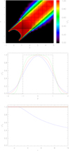 |
Fig. 3. Searchlight-beam test for direction n = (1, 0, 1) and a typical grid with Nx = Ny = Nz = 133 grid points. Upper panel: contour plot of the specific intensity as calculated with the SC method using Bézier interpolations in the xz-plane (cf. Paper I, Fig. 3, for the finite-volume method). Middle panel: specific intensity through the perpendicular area indicated by the straight line in the upper panel. The blue, red, and green profiles correspond to the FVM, SClin, and SCbez methods, respectively. The dashed line indicates the theoretical profile. Bottom panel: as middle panel, but along the centre of the searchlight beam. We note that the SC methods reproduce the exact solution at the centre of the beam, whereas the FVM solution decreases significantly for r ≳ 2.5 R*. |
Along the beam centre, the SC methods perfectly reproduce the exact solution, whereas the FVM solution decreases significantly due to the finite grid-cell size (see Paper I). Considering the intensity through the perpendicular area, both SC methods perform better than the FVM, with slight advantages of the SCbez method when compared with the SClin method. Within the 3D SC methods, however, energy conservation is violated for our zero opacity models, because the (nominal) specific intensity jumps from  to zero for rays intersecting the stellar surface or not, due to the core-halo approximation. As a consequence, almost all interpolations (and interpolation schemes) overestimate the specific intensity5. For optically thick models (where
  at the core plays a negligible or minor role), this effect should decrease though. The associated error can be quantified by calculating the corresponding flux, that is, by integrating the specific intensity for a given direction over a corresponding perpendicular area (defined as a circle with virtually infinite radius). We emphasize that the flux as defined here constitutes the most demanding test case, and should not be confused with the flux density (i.e. the first moment of the specific intensity). Figure 4 shows the resulting fluxes (normalized by the nominal value) for searchlight beams with different directions defined by θ = 45° and ϕ ∈ [0° ,90° ]. For different directions ϕ, the searchlight beams propagate through different domains of the spatial grid with accordingly different grid-cell sizes. Due to the distinct behaviour of numerical diffusion errors within these domains, the total flux varies as a function of ϕ. Overall, the total fluxes for the SClin and SCbez methods are larger than theoretically constrained, whereas the FVM gives (despite a small error) reasonable results. This effect is largest in regions far from the star and for diagonal directions. Thus, particularly in these regions, also the mean intensities (for optically thin atmospheres) are expected to be overestimated. The same problem arises when calculating line transitions, since photons may freely propagate over large distances before a resonance region is hit. Numerical diffusion errors can only be avoided by increasing the grid resolution, or using higher order upwind-interpolation methods.
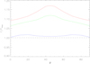 |
Fig. 4. Photon flux as a function of direction angle ϕ (with fixed θ = 45°) through corresponding perpendicular areas, and with the opacity set to zero. The central distance of all areas to the stellar surface has been set to 2 R*. The same colour coding as in Fig. 3 has been used. |
4.2. Spherically symmetric stellar winds
In this section, we test the performance of the 3D SC method when applied to spherically symmetric, stationary atmospheres. For consistency, the same test models as in Paper I have been calculated, with the wind described by a β-velocity law and the continuity equation:
For stellar and wind parameters, R* = 19 R⊙, Ṁ = 5 × 10⁻⁶ M⊙ yr−1, β = 1, vmin = 10 km s−1, v∞ = 2000 km s−1, the density stratification and the velocity field are completely determined. For the considered scattering problems (ϵC = ϵL = 10−6), effects of the temperature stratification are negligible. The continuum and (frequency integrated) line opacities have been calculated from Eqs. (7) and (8), with the electron density derived for a completely ionized H/He plasma with helium abundance NHe/NH = 0.1. We have calculated three different continuum models by scaling the opacity with kC = [1, 10, 100], respectively. These models correspond to an optically thin, marginally optically thick, and optically thick atmosphere, with radial optical depths τr = [0.17, 1.7, 17]. The line transport has been calculated for a weak, intermediate, and strong line, with line-strengths kL = [1, 103, 105]. To minimize the computation time, we use a microturbulent velocity vmicro = 100 km s−1 throughout this paper. Such a large velocity dispersion mimicks the effects of multiply non-monotonic velocity fields resulting from the line-driven instability (Paper I and references therein). The atomic mass has been set to mA = 12 mp. Finally, the emergent intensity from the stellar core is calculated from Trad = Teff = 40 kK.
4.2.1. Convergence behaviour
Figure 5 shows the maximum relative corrections of the mean intensity (left panel) and scattering integral (right panel) after each iteration step. Different methods (SClin, SCbez, and FVM), and different acceleration techniques (classical Λ-iteration, and diagonal-, direct-neighbour-, nearest-neighbour-ALO with the Ng-extrapolation switched on or off) have been applied. We display the continuum and line calculations for kC = [10, 100] and kL = [10, 105], respectively, using Nx = Ny = Nz = 93 spatial and NΩ = 974 angular grid points (to save computation time when calculating the slowly converging classical Λ-iteration). In the following, we only discuss the convergence behaviour of the SClin and SCbez methods, as the FVM has already been analysed in Paper I. We usually stop the iteration scheme when the maximum relative corrections become less than 10−3 between subsequent iteration steps, emphasizing that a truly converged solution is only found when the curve describing subsequent relative corrections is sufficiently steep6. For instance, the classical Λ-iteration (with Λ* = 0) fails to converge for strong scattering lines (Fig. 5, lower right panel), since the relative corrections become almost constant in each iteration step (“false convergence”, cf. Hubeny & Mihalas 2014).
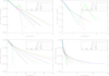 |
Fig. 5. Convergence behaviour of the standard spherically symmetric model calculated with the 3D FVM (blue) and the 3D SC method using linear (red) or Bézier (green) interpolations. Left and right panels: convergence behaviour of the continuum and line transfer for ϵC = ϵL = 10−6, respectively. While the upper row displays the optically thin models with kC = 10 and kL = 10, the lower row has been calculated using kC = 100 and kL = 105. Different acceleration techniques have been applied, where the NN-ALO is implemented only for the SC method. |
Overall, and as expected, the number of iterations needed to obtain the converged solution is decreasing with increasing number of matrix elements used to define the ALO (see also Hauschildt et al. 1994; Hauschildt & Baron 2006 for multi-band ALOs coupled to a 1D-SC and 3D-LC formal solution scheme, respectively). In most cases, the convergence of the SClin is faster than that of the SCbez method, because the interpolation scheme is intrinsically more localized (with stronger weights assigned to local Λ-matrix elements). The FVM always performs best, since only the direct neighbours directly influence the formal solution within this method.
For parameters kC, kL ≤ 10 (Fig. 5, upper panels), all ALOs yield a converged solution within Niter ≈ 10 iteration steps. When applying the SCbez method, the first peak results from switching the linear interpolations to Bézier interpolations at the fifth iteration step. This peak is less pronounced for parameters kC, kL = 100, 105, since the maximum relative corrections are still relatively large in the first few iteration steps.
For the optically thick continuum model (Fig. 5, lower left panel), the number of iterations until convergence is reduced from  to
to  and
and  when using the diagonal, DN-, and NN-ALO within the SClin and SCbez method, respectively. The Ng-extrapolation significantly reduces Niter further, and is required to obtain the converged solution in ≲20 iteration steps.
For the strong line, the convergence behaviour becomes slightly improved, because the radiative transfer is localized to (narrow) resonance regions. Thus, already the diagonal and DN-ALO yield a solution within  and
and  iteration steps. Again, the NN-ALO with the Ng-extrapolation scheme switched on performs best, and reduces the number of iteration steps until convergence to ≲20.
In total, we conclude that a NN-ALO together with the Ng-extrapolation is required for the SClin and SCbez methods, in order to obtain a fast convergence behaviour of the iteration scheme. This ALO also performs excellently for extreme test-cases, that is, for optically thick continua and strong lines in scattering dominated atmospheres.
4.2.2. Continuum and line solution
In the following, we discuss the errors resulting from the upwind and downwind interpolations, and from the integration of the discretized radiative transfer equation. We apply the NN-ALO together with the Ng-extrapolation to ensure convergence. When calculating the line, we used Nx = Ny = Nz = 93 spatial grid points. Since the continuum transport has been calculated at only one frequency point, we applied a higher grid resolution with Nx = Ny = Nz = 133 for such problems. Figure 6 shows the continuum and line solutions together with corresponding relative errors obtained for the spherically symmetric model when calculated with the FVM, SClin, and SCbez methods, and compared to the “exact” 1D solution. The mean and maximum relative errors are shown for different regions in Table 2, where the mean and maximum relative errors of any quantity are defined throughout this paper by
![Mathematical equation: $$ \begin{aligned}&\overline{\Delta q} := \dfrac{1}{N} \sum _{i=1}^N \dfrac{|q_i-q_i^\mathrm{(exact)}|}{q_i^\mathrm{(exact)}} \nonumber \\&\Delta q_{\rm max} := \max \limits _{\forall i \in [1,N]} \dfrac{|q_i-q_i^\mathrm{(exact)}|}{q_i^\mathrm{(exact)}},\nonumber \end{aligned} $$](/articles/aa/full_html/2020/01/aa36584-19/aa36584-19-eq90.gif)
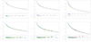 |
Fig. 6. Solutions for the standard spherically symmetric models as calculated with the 3D FVM (blue) and 3D SC methods using linear (red) or Bézier (green) interpolations, compared to an accurate 1D solution (black solid line). The dots represent the solutions at specific grid points (with different latitudes and longitudes), where only a subset of all grid points is displayed to compress the image. Corresponding errors are indicated at the bottom of each chart. Top panel: mean intensity for the continuum transfer as a function of radius, with ϵC = 10−6, and kC = [1, 10, 100] from left to right. Bottom panel: line source function with ϵL = 10−6, and kL = [100, 103, 105] from left to right. |
Mean and maximum relative errors of the FVM and SClin, SCbez methods, when applied to spherically symmetric test models.
with N the number of grid points within the considered region.
For the continuum models, the solutions obtained from the 3D SC methods are superior to the solution obtained from the FVM in most cases. Particularly near the stellar surface (at r ≲ 3 R*), both SC methods are in good agreement with the 1D solution (see Fig. 6, top panel, and bottom of each chart for the radial dependence of the relative errors). When considering the most challenging problem of optically thick, scattering dominated atmospheres, the mean relative errors of the SClin and SCbez method for the complete calculation region are on the 20- and 10%-level, respectively. For such models, the FVM breaks down due to the order of accuracy (see Paper I), and a (high order) SC method is indeed required to solve the radiative transfer with reasonable accuracy. For marginally optically thick continua, the mean relative errors of the SClin and SCbez methods are on the 5%-level and below. While the FVM allows for a qualitative interpretation of the radiation field for such models, the SC methods should be used for quantitative discussions. The optically thin model calculations give mean relative errors of the order of 5% for all methods, with the maximum relative error being lowest for the FVM. Since, additionally, the computation times of the SClin and SCbez methods are typically highest (see Sect. 3.7), the FVM is to be preferred when calculating optically thin continua. We note that all errors originate from the interplay between upwind and downwind interpolations of opacities, source functions, and intensities, and from the integration of the discretized radiative transfer equation. Numerical diffusion and the associated violation of energy conservation influences the converged solution particularly in the optically thin regime.
The mean relative errors for the line transition are of the order of 5 − 10%, with increasing accuracy from strong to weak lines, and slight advantages of the SCbez method when compared to the SClin method. The radial stratification of relative errors for each considered line is shown in the bottom panel of Fig. 6, bottom of each chart. While the FVM gives largest errors near the stellar surface (at r ≲ 3 R*), both SC techniques are in excellent agreement with the 1D solution in such regions. At larger radii, however, the SC solutions are generally overestimated when compared to the 1D solution due to numerical diffusion errors. The distinct behaviour of the applied solution schemes in different atmospheric regions finally determines the quality of emergent flux profiles.
4.2.3. Emergent flux profile
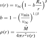
The converged source functions are used to calculate the emergent flux profile using the same postprocessing LC solver as in Paper I. Based on Lamers et al. (1987), Busche & Hillier (2005), and Sundqvist et al. (2012), this method solves the equation of radiative transfer in cylindrical coordinates with the z-axis being aligned with the line of sight of the observer’s direction under consideration. All quantities required on the rays are found by trilinear interpolation from the 3D grid, and the equation of radiative transfer is integrated using linear interpolations. To extract the error resulting from the FVM and SC methods alone, we interpolated the “exact” 1D solution onto our 3D grid and calculated the reference profile using the same technique. The continuum has been calculated from a zero-opacity model given by the unattenuated illumination from the projected stellar disc. Then, the differences of line profiles are exclusively related to the differences of line source functions. Figure 7 shows the line profiles with corresponding absolute and relative errors for the intermediate (kL = 103) and strong (kL = 105) line, obtained from the converged source functions from above.
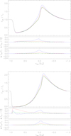 |
Fig. 7. Emergent flux profiles of an intermediate (kL = 103, top panel) and strong (kL = 105, bottom panel) line. The blue, red, and green curves correspond to the solution of the FVM, SClin, and SCbez methods, respectively. The reference profile (black solid line) has been derived from the “exact” 1D source function interpolated onto the 3D Cartesian grid. Corresponding relative and absolute errors are shown at the bottom of each chart. For all profiles, the continuum level has been determined from a zero-opacity model. |
The line profiles are in good agreement with the 1D solution for both applied SC methods, with slight advantages of the SCbez method when compared to the SClin. Major (relative) deviations arise particularly at large frequency shifts on the blue side due to the enlarged source functions in corresponding resonance regions (i.e. at large radii in front of the star). At such frequency shifts, however, the line profile is mainly controlled by absorption, and the absolute error remains small. At low frequency shifts, the emission peak becomes slightly overestimated, particularly when considering the strong line. The corresponding resonance regions are mainly located near to the star (at low absolute velocities) and in the whole plane perpendicular to the line of sight (with low projected velocities). For the intermediate line, the emission from this plane at large radii only plays a minor role due to relatively small optical-depth increments along the line of sight. Thus, both SC methods are in excellent agreement with the 1D reference profile. With increasing line strength, however, the emission from the outer wind region contributes significantly to the line formation, and the discrepancies between the 1D and the SClin/SCbez methods become more pronounced. For all test calculations, the Bézier method performs best, closely followed by the SClin method, and (far behind) the FVM.
With Fig. 7 and the argumentation from above, we conclude that (at least) a short-characteristics solution scheme is required to enable a quantitative interpretation of ultra-violet (UV) resonance line profiles, where both the linear and Bézier interpolation techniques perform similarly well. The less accurate (however computationally cheaper) FVM can still be applied for qualitative discussions.
5. Rotating winds
As a first application of the 3D SC method to non-spherical atmospheres, we consider the UV resonance line formation in the winds of (fast) rotating O stars. Fast rotation has two immediate consequences on the stellar geometry and wind structure. Firstly, the surface of any rotating star becomes distorted, with Req/Rpole approaching 3/2 for rotational speeds near the critical velocity (Collins 1963 assuming a Roche model, and the critical velocity defined by Eq. (36) for Ω = 1). Secondly, the emergent flux depends on the (local) effective gravity (corrected for the centrifugal acceleration), and thus, decreases towards the equator (“gravity darkening”, see von Zeipel 1924; Maeder 1999; Maeder & Meynet 2000 for uniform and shellular rotation, respectively). The first attempt to model the winds of fast rotating OB stars was made by Bjorkman & Cassinelli (1993). These authors considered a purely radial line force, and neglected gravity darkening and the surface distortion. Within these approximations, a “wind compressed disc” is formed in the equatorial plane. Cranmer & Owocki (1995) and Owocki et al. (1996) included the effects of non-radial line-forces into their 2D radiation-hydrodynamic simulations, and showed that the formation of the disc becomes suppressed due to a small, but significant polewards acceleration, giving rise to an associated polar velocity component that prevents the formation of a disc. When also accounting for gravity darkening (i.e. a decreased radial acceleration in equatorial regions), Owocki et al. (1996) further showed that a prolate wind structure develops, with decreased equatorial mass loss and velocity (see also the review by Owocki et al. 1998). Maeder (1999) proposed that an oblate wind structure might still be possible, when accounting for a polar variation of the ionization equilibrium induced by gravity darkening (the so-called κ-effect). This effect becomes particularly important when the local effective temperature drops below the bi-stability jump temperature7. Petrenz & Puls (2000) extended the hydrodynamic calculations from above by allowing for spatially varying line force multipliers, and showed that no major differences from the prolate wind structure arise, at least for OB stars above Teff ≳ 20 kK with an optically thin Lyman continuum. Recently, Gagnier et al. (2019) reinvestigated the effects of rotation using 2D ESTER models (see Rieutord et al. 2016 for a description of this code). Using a different implementation of gravity darkening (consistent with the so-called ω-model by Espinosa Lara & Rieutord 2011, which basically results in a slower decrease of effective temperature with co-latitude than obtained from the von Zeipel theorem), these authors predict either a “single-wind regime” (with enhanced polar mass loss) or a “two-wind regime” (with enhanced mass loss at latitudes where the effective temperature drops below the bi-stability jump temperature). To understand which of the different models represents reality best (in different temperature regimes), one needs to compare synthetic profiles with observations. In this respect, investigating the effects of prolate and oblate wind structures is particularly important to distinguish between different theories.
As a consequence of the distinct wind structure resulting from a particular model, the wind lines of rotating stars are expected to differ as a function of rotational speed and inclination. To predict UV resonance line profiles of fast rotating stars, we calculated the source function of a prototypical resonance line transition including the effects of gravity darkening and surface distortion for models with different rotational velocities. As a first step, we used a wind description that is consistent with the prolate wind model. For all calculations, we applied the SClin method.
5.1. Wind model
To obtain a model for the structure of rotating winds, we applied a 2D version of the VH-1 code8 developed by J. M. Blondin and co-workers. Our model includes the effects of gravity darkening and surface distortion (see below). Using a 1D input model derived from radiation driven wind theory including finite cone angle corrections (Castor et al. 1975; Pauldrach et al. 1986) for the first time step, the radiation hydrodynamic equations (accounting for non-radial line forces) are solved until a (quasi) stationary solution is obtained (see Cranmer & Owocki 1995; Owocki et al. 1996 for the description of the line force). Assuming azimuthal symmetry, the resulting 2D density and velocity structure is then used as input for our 3D SC code. Table 3 summarizes specific parameters used and obtained for our model calculations. While the surface integrated mass flux, Ṁ, becomes only slightly increased with increasing rotational speed, the polar (equatorial) terminal velocities are significantly enhanced (reduced). For the fastest rotating model (vrot = 432 km s−1), Fig. 8 shows corresponding density contours in the xz-plane. The z-axis is aligned with the rotation axis. To explicitly show the prolate wind structure, we have scaled the density by the density resulting from the non-rotating (spherically symmetric) model, as a function of distance from the stellar surface. For different rotational speeds, Fig. 9 displays the density and radial velocity along the polar axis and along an (arbitrarily defined) axis in the equatorial plane. When compared with the spherically symmetric wind, the densities of the rotating models are enhanced in polar regions, and become reduced along the equator. Further, the radial velocity along the polar axis remains nearly the same, except in regions far from the star, where the terminal velocity of all rotating models becomes enhanced with increasing vrot. We note that one would expect clearer differences of the (radial) velocity fields for different rotation rates, due to different accelerations induced, particularly, by the different radiative fluxes resulting from gravity darkening, and, though to a lesser extent, by the specific density structure and rotational velocities. Such differences can be barely observed within our simulations, most presumably because the wind structure in polar regions has not completely settled to a stationary state at the last time steps. In contrast, the radial velocity in equatorial regions is significantly reduced at all distances, when compared to the non-rotating wind, and the deviations from spherical symmetry become more pronounced with increasing rotational velocity. Although we have averaged the hydrodynamic simulations over the last 20 time steps, the atmospheric structure still suffers from small numerical artefacts.
 |
Fig. 8. Contours of the density in the xz-plane (z being the rotation axis) for a prototypical rotating O star with L* = 106 L⊙, M* = 52.5 M⊙, Rp = 19 R⊙, and vrot = 432 km s−1 (corresponding to Ω = 0.9). The density has been scaled by values from the non-rotating model with Ω = 0. While the thick solid line corresponds to the surface of the (distorted) star, the dashed line would correspond to a spherical surface. Additionally, the velocity vectors are displayed. |
 |
Fig. 9. Density and radial velocity as a function of distance from the stellar surface in polar (first and third panel) and equatorial (second and fourth panel) regions, for different rotation parameters Ω. |
Specific parameters used and obtained for the rotating wind models.
To calculate the stellar surface distortion, we consider the gravitational potential of the star accounting for the effects of centrifugal forces. Under reasonable assumptions, we can approximate this potential by a Roche model (e.g. Collins 1963, see also Cranmer & Owocki 1995):
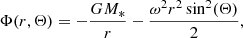 (34)
(34)
with angular velocity ω. The surface of the star is defined on equipotential lines and can be calculated by setting Φ(Rp, Θ = 0) = Φ(R*(Θ),Θ), with Rp the polar radius. Solving the resulting cubic equation, one finds:
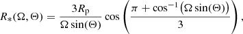 (35)
(35)
with Ω = ω/ωcrit the ratio of the actual to the critical (“breakup”) angular velocity. Defining the rotational speed at the equator vrot as input parameter, one easily obtains (cf. Cranmer & Owocki 1995, their Eq. (27)):
 (36)
(36)
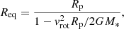 (37)
(37)
with equatorial radius Req. Following Maeder & Meynet (2000), we use the actual stellar mass to calculate the equatorial radius and critical velocity without correcting for Thomson-accelerations. Additionally, we note that our stellar models are well below the Eddington limit (Γ = 0.5). Thus, the critical angular velocity is simply given by 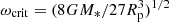 . Instead of using Eq. (35) in our final implementation, we approximated the stellar surface by a spheroid with semi-major axes a = b = Req and semi-minor axis c = Rp. Such a formulation greatly simplifies the calculation of the intersection of a given ray with the stellar surface (required for the boundary conditions, see Sect. 3.4). For the most extreme test case considered here (Ω = 0.9), the maximum error on R*(Θ) due to this approximation is well below the 2%-level, and rapidly decreases for lower rotational velocities.
To calculate the intensity emerging from the stellar core, we set  , with the effective temperature as a function of co-latitude. For a given luminosity of the star, L*, we obtain (see also Petrenz & Puls 1996):
![Mathematical equation: $$ \begin{aligned}&T_{\rm eff}(\Theta ) = \Bigl [ \dfrac{L_{*}}{2 \pi \sigma _{\rm B}\Sigma }|{\boldsymbol{g}} |^{4\beta _{Z}} \Bigr ]^{1/4}\nonumber \\&\Sigma = \int _0^\pi |{\boldsymbol{g}} |^{4\beta _{Z}} \dfrac{R_{*}^2(\Theta )\sin (\Theta )}{- g_r/|{\boldsymbol{g}} |} \mathrm{d}\Theta , \end{aligned} $$](/articles/aa/full_html/2020/01/aa36584-19/aa36584-19-eq103.gif) (38)
(38)
with σB the Stefan Boltzmann constant, and the surface integrated effective gravity Σ derived from g(Θ) = − ∇Φ(R*(Θ),Θ). The parameter βZ describes the gravity darkening law in terms of Teff(Θ)∝|g(Θ)|βZ. As originally formulated by von Zeipel (1924), βZ = 1/4. Though βZ might be significantly lower (e.g. Domiciano de Souza et al. 2014; Gagnier et al. 2019), for simplicity we nevertheless used βZ = 1/4. As long as we assume constant ionization fractions, the effect of βZ on the line profiles will be minor anyway.
5.2. Line formation
For our test models, we used vmicro = 100 km s−1, and calculated the frequency integrated opacity from Eq. (8) for an intermediate and a strong line with line-strength parameter kL = 103 and kL = 105. To obtain the source function, we applied the 3D SClin method and set ϵL = 10−6. The resulting (normalized) line profiles are shown in Fig. 10 for different rotational velocities and inclination angles. Additionally, we display the continuum flux used for normalization in Fig. 11. Due to gravity darkening and the surface distortion, the continuum depends on the rotation rate and inclination, with largest fluxes found for high rotation rates and low inclinations (resulting from the higher temperatures in polar regions and a larger projected stellar disc). In Figs. 10 and 11, the x-axes have been normalized to an (arbitrarily chosen) terminal velocity v∞ = 3000 km s−1. The behaviour of the line profiles can be qualitatively explained with the hydrodynamic structure:
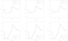 |
Fig. 10. Predicted emergent flux profiles for the rotating star models with Ω = [0, 0.5, 0.7, 0.9] (see Table 3). Upper and lower panels: intermediate and strong line with kL = 103 and kL = 105, respectively. The inclination angle has been set to sin(i) = [0, 0.707, 1] from left to right. |
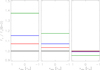 |
Fig. 11. Continuum fluxes for different inclinations sin(i) = [0, 0.707, 1] from left to right, and different rotation parameters (using the same colour coding as in Fig. 10). The continuum fluxes have been scaled by the corresponding flux obtained from the non-rotating model. |
-
(i)
For pole on observers (sin(i) = 0, left panel of Fig. 10), the absorption column in front of the star is enhanced with increasing rotational velocity due to the larger densities (and opacities) in polar regions. Thus, the absorption trough (of unsaturated lines) becomes more pronounced. The absorption edge of the intermediate lines is found at slightly lower velocities than expected from the hydrodynamic simulations, because the optical depths of the corresponding resonance regions are too low to efficiently contribute to the absorption. When considering the strong lines, the optical depth is larger, and the absorption edge is more consistent with the actual terminal velocity. For both applied line strength parameters, the emission peak becomes weaker with increasing rotation rate, particularly at low projected velocities on the red side of the line centre (for negative xobs). This effect can be partly explained by the reduced emission from the equatorial plane, due to the lower densities in these regions. More importantly, however, is the increased continuum flux that mainly determines the (normalized) height of the emission peak.
-
(ii)
When increasing the inclination towards equator-on observers (sin(i) = 1, right panel of Fig. 10), the behaviour is reversed. For such directions, the continuum plays an only minor role, since the lower (equatorial) effective temperatures of the rotating models are nearly compensated by the enlarged projected stellar disc. With increasing rotation parameter, the absorption trough of the intermediate line becomes reduced and shifted towards lower terminal velocities, consistent with the hydrodynamical model. When considering the strong line, the absorption becomes saturated, and only the impact of the different terminal velocities can be observed. Additionally, and for both line strengths, the absorption slightly extends towards the red side, because of (negative) projected line of sight velocities near the stellar surface induced by rotation. For the fastest rotating model with Ω = 0.9, this effect becomes suppressed due to an increased emission from the (dense) prolate wind structure. This latter effect is only moderate for lower rotational speeds. Based on the current hydrodynamic wind structure, we would therefore expect to observe either rather low terminal velocities or relatively deep absorption troughs for fast rotating stars, and we are able, at least in principle, to check the theory by comparing our synthetic spectra with (past or future) UV observations. This point, however, is beyond the scope of this paper.
Finally, if the projected rotational velocity is known (e.g. from photospheric lines), one might even estimate the actual rotational velocity from UV resonance lines. This latter point becomes clear from Fig. 12, where we predict the line profiles of models with different rotational speed for a given v sin (i) (set here to 200 km s−1). Since, at least for the intermediate line, the profile shapes differ, sin (i) could be derived if v sin (i) was known. Of course, such constraints will become feasible only if the underlying models correctly describe the wind structure (including possibly varying ionization stages) of rotating stars.
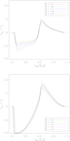 |
Fig. 12. Predicted emergent flux profiles for the rotating star models with Ω = [0.5, 0.6, 0.7, 0.8, 0.9], and different inclination angles such that v sin (i) = 200 km s−1 for all models. The upper and lower panels display the intermediate (kL = 103) and strong (kL = 105) line, respectively. |
6. Summary and conclusions
In this study, we have presented a 3D short-characteristics method tailored for the solution of continuum- and line-scattering problems in the winds of hot stars. To obtain the formal solution, we have implemented a purely linear interpolation scheme (for calculating upwind quantities and for the solution of the radiative transfer equation along a ray), as well as a second order, monotonic, Bézier technique. We use Cartesian coordinates with a non-uniform grid spacing to ensure a reasonable spatial resolution in important regions (i.e. where velocity and/or density gradients are large). As a first step towards full NLTE radiative transfer models, we consider a single resonance-line transition (approximated by a two-level-atom) assuming an optically thin background continuum, whereas for pure continuum problems we use the thermalization parameter, ϵC, and split the source function into a scattering and a thermal part. A generalization (including multi-level atoms) is planned for future applications.
To calculate strong scattering lines and optically thick, scattering dominated continua, we have implemented an accelerated Λ-iteration scheme using different non-local approximate Λ-operators (ALOs), together with applying the Ng-extrapolation method for subsequent iterations. With increasing complexity of the ALO (i.e. from a purely diagonal ALO to a nearest-neighbour ALO including also the 26 neighbouring terms), the rate of convergence is improved. When applying the NN-ALO, the converged solution is generally found within ≲20 iteration steps even for the most challenging test cases.
We have estimated the error of the applied methods in different regimes by calculating spherically symmetric test models within our 3D SC framework, and with a 3D finite-volume method. To our knowledge, this is the first study, where different 3D solution schemes for spherical problems have been compared, and their precision explored. When rated against the solution obtained from (accurate) 1D solvers, we found a mean relative error for the converged continuum source function of roughly 5 − 10% and 5 − 20% when using Bézier and linear interpolations, respectively. Particularly for optically thick continua, the (first order) FVM method breaks down, and a (high order) SC or LC method is required to accurately solve the radiative transfer. When considering the solution of the line source function for different line-strength parameters, the mean relative errors of both SC methods are on the 10%-level and below, with slight advantages of the Bézier technique compared to purely linear interpolations. The resulting synthetic line profiles are calculated with a long-characteristics postprocessing routine using the previously calculated converged source functions. The SC method using Bézier interpolations almost perfectly matches the 1D reference profiles for all our models (i.e. for weak and strong lines). When linear interpolations are used, we obtain slight deviations originating mainly in the outer wind regions. In contrast, the 3D FVM always overestimates the emission. Nevertheless, all methods have their own advantages and disadvantages, particularly when also accounting for the computation time (with fastest turn-around times for the FVM method). Thus, the 3D FVM method should be used for qualitative interpretations and for finding (rough) estimates of the parameters of interest, while the SC methods are to be preferred when aiming at a quantitative analysis of line profiles, and for optically thick continua.
As a first application of the 3D SC code to non-spherical problems, we considered the resonance line formation in the winds of (fast) rotating O stars. Assuming azimuthal symmetry, the hydrodynamic structure for a prototypical O star with different rotation rates has been calculated by means of the 2D VH-1 code. We have included the effects of surface distortion and gravity darkening into our 3D radiative transfer framework. Given the hydrodynamic models, we are able to predict the shape of line profiles for different rotational speeds and inclination angles. When compared with a (non-rotating) spherically symmetric wind (obtained using the same stellar parameters), rotating stars should either show relatively low terminal velocities (for equator-on observers) or deeper absorption troughs (for pole-on observers). The latter effect, however, would only be observable when considering intermediate (i.e. unsaturated) lines. Additionally, we showed that the line profile shapes vary as a function of rotational speed at a given v sin (i). Thus, assuming that v sin (i) was known (e.g. from photospheric line modelling), one could estimate the rotational speed, though with a rather large uncertainty, since the differences of the line profiles are only moderate. We emphasize that other effects (such as clumping or a flatter gravity darkening law) may additionally shape the line profiles. When analysing UV observations of fast rotating stars, the 3D SC code developed in this work certainly will help to understand the manifestations of various (aforementioned) effects, and to distinguish between different theoretical predictions (e.g. prolate vs. oblate wind structures). Ideal testbeds for future investigations of fast rotating winds are the stars VFTS102 (O9 Vnnne, Dufton et al. 2011) and VFTS285 (O7.5 Vnnn, Walborn et al. 2012), both rotating at nearly their critical velocity.
Finally, we note that our tools are, of course, not limited to rotating stars. Indeed, almost any kind of stellar wind that deviates from spherical symmetry (with non-relativistic velocity fields), such as magnetic winds or colliding winds in close binaries, can be investigated.
In this paper, different interpolation schemes are tested by considering simplified (though physically relevant) continuum and line scattering problems. We emphasize that our code will be further developed to enable the solution of more complex, multi-level problems in 3D. For such problems, highly accurate interpolation schemes are required to describe the variation of the mean intensities along a ray.
For a given grid point, the number of neighbouring grid points that can be used for extrapolation is not a priori clear, and depends on the shape of the stellar surface, and the considered direction of the ray. Indeed, there are 64 special cases that would have to be implemented explicitly. This is computationally not feasible.
For the simplified continuum and the TLA considered in this paper, the linear interpolation scheme is particularly advantageous in terms of computation time, since the corresponding ALO remains constant over all iteration steps, and therefore needs to be calculated only once.
The 1D solution for the continuum transport is found from the Rybicki-algorithm (combined with the solution of the moment equations using variable Eddington factors, see, e.g. Mihalas 1978). To calculate the line, a comoving-frame ray-by-ray solution scheme in pz-geometry is applied, ensuring convergence with a diagonal ALO.
In contrast, the number of photons entering and leaving a given grid cell is (nearly) conserved within the FVM by definition. This statement, however, is not completely true for the FVM as formulated by Adam (1990), Lobel & Blomme (2008), and Hennicker et al. (2018), since all these authors apply an (averaged) upwind approximation.
For linearly convergent iteration schemes, the steepness of the convergence curve is described by the relative corrections in subsequent iterations steps, Δk/Δk − 1 = const. = :q. To obtain a solution within a reasonable amount of computation time, we may demand that q ≲ 0.8, corresponding to a reduction of relative errors by a factor of 10−3 every 30th iteration step.
The jump temperature is theoretically motivated by a stronger radiative line-driving due to lower ionization stages of iron for Teff ≲ Tjump ≈ 25 kK (Vink et al. 1999). More recently, Petrov et al. (2016) predicted a somewhat lower jump temperature, Tjump ≈ 20 kK.
If xc was located at xc = xi − 1 + 3/4(xi − xi − 1), for instance, one can easily show that the resulting Bézier curve never reproduces the unit parabola for any ordinate value fc.
Sp ≠ 0 only when considering the grid point p ↔ (ijk). Then,  , and
, and  only when the upwind point is located on the stellar surface (Eq. (D.14)).
Acknowledgments
We thank our referee, Dr. Achim Feldmeier, for many helpful comments and suggestions, that improved the first version of this manuscript considerably. LH gratefully acknowledges support from the German Research Foundation, DFG, under grant PU 117/9-1. NDK acknowledges funding from the KU Leuven C1 grant MAESTRO C16/17/007. JOS acknowledges support from FWO Odysseus grant D4545-GH9218. Finally, we thank J. M. Blondin and co-workers for providing the VH-1 code.
References
- Abbott, B. P., Abbott, R., Abbott, T. D., et al. 2016, Phys. Rev. Lett., 116, 061102 [Google Scholar]
- Adam, J. 1990, A&A, 240, 541 [NASA ADS] [Google Scholar]
- Ahrens, C., & Beylkin, G. 2009, Proc. R. Soc. A: Math. Phys. Eng. Sci., 465 [Google Scholar]
- Auer, L. 2003, in Stellar Atmosphere Modeling, eds. I. Hubeny, D. Mihalas, & K. Werner, ASP Conf. Ser., 288, 3 [NASA ADS] [Google Scholar]
- Beentjes, C. H. L. 2015, Quadrature on a Spherical Surface (Oxford: University of Oxford) [Google Scholar]
- Bjorkman, J. E., & Cassinelli, J. P. 1993, ApJ, 409, 429 [NASA ADS] [CrossRef] [Google Scholar]
- Busche, J. R., & Hillier, D. J. 2005, AJ, 129, 454 [NASA ADS] [CrossRef] [Google Scholar]
- Cannon, C. J. 1973, ApJ, 185, 621 [NASA ADS] [CrossRef] [Google Scholar]
- Castor, J. I., Abbott, D. C., & Klein, R. I. 1975, ApJ, 195, 157 [NASA ADS] [CrossRef] [Google Scholar]
- Cherepashchuk, A. M. 1976, Sov. Astron. Lett., 2, 138 [NASA ADS] [Google Scholar]
- Collins, II., G. W. 1963, ApJ, 138, 1134 [NASA ADS] [CrossRef] [Google Scholar]
- Cranmer, S. R., & Owocki, S. P. 1995, ApJ, 440, 308 [NASA ADS] [CrossRef] [Google Scholar]
- David-Uraz, A., Erba, C., Petit, V., et al. 2019, MNRAS, 483, 2814 [NASA ADS] [CrossRef] [Google Scholar]
- de Mink, S. E., Langer, N., Izzard, R. G., Sana, H., & de Koter, A. 2013, ApJ, 764, 166 [NASA ADS] [CrossRef] [Google Scholar]
- Domiciano de Souza, A., Kervella, P., Moser Faes, D., et al. 2014, A&A, 569, A10 [NASA ADS] [CrossRef] [EDP Sciences] [Google Scholar]
- Dufton, P. L., Dunstall, P. R., Evans, C. J., et al. 2011, ApJ, 743, L22 [NASA ADS] [CrossRef] [Google Scholar]
- Dullemond, C. P., & Turolla, R. 2000, A&A, 360, 1187 [NASA ADS] [Google Scholar]
- Espinosa Lara, F., & Rieutord, M. 2011, A&A, 533, A43 [NASA ADS] [CrossRef] [EDP Sciences] [Google Scholar]
- Gagnier, D., Rieutord, M., Charbonnel, C., Putigny, G., & Espinosa Lara, F. 2019, A&A, 625, A88 [NASA ADS] [CrossRef] [EDP Sciences] [Google Scholar]
- Georgiev, L. N., Hillier, D. J., & Zsargó, J. 2006, A&A, 458, 597 [NASA ADS] [CrossRef] [EDP Sciences] [Google Scholar]
- Gräfener, G., Koesterke, L., & Hamann, W.-R. 2002, A&A, 387, 244 [NASA ADS] [CrossRef] [EDP Sciences] [Google Scholar]
- Hauschildt, P. H. 1992, J. Quant. Spec. Radiat. Transf., 47, 433 [Google Scholar]
- Hauschildt, P. H., & Baron, E. 2006, A&A, 451, 273 [NASA ADS] [CrossRef] [EDP Sciences] [Google Scholar]
- Hauschildt, P. H., Störzer, H., & Baron, E. 1994, J. Quant. Spec. Radiat. Transf., 51, 875 [NASA ADS] [CrossRef] [Google Scholar]
- Hayek, W., Asplund, M., Carlsson, M., et al. 2010, A&A, 517, A49 [NASA ADS] [CrossRef] [EDP Sciences] [Google Scholar]
- Heger, A., Fryer, C. L., Woosley, S. E., Langer, N., & Hartmann, D. H. 2003, ApJ, 591, 288 [NASA ADS] [CrossRef] [Google Scholar]
- Hennicker, L., Puls, J., Kee, N. D., & Sundqvist, J. O. 2018, A&A, 616, A140 [NASA ADS] [CrossRef] [EDP Sciences] [Google Scholar]
- Hillier, D. J., & Miller, D. L. 1998, ApJ, 496, 407 [NASA ADS] [CrossRef] [Google Scholar]
- Holzreuter, R., & Solanki, S. K. 2012, A&A, 547, A46 [NASA ADS] [CrossRef] [EDP Sciences] [Google Scholar]
- Hubeny, I., & Mihalas, D. 2014, Theory of Stellar Atmospheres (Princeton: Princeton University Press) [Google Scholar]
- Ibgui, L., Hubeny, I., Lanz, T., & Stehlé, C. 2013, A&A, 549, A126 [NASA ADS] [CrossRef] [EDP Sciences] [Google Scholar]
- Jones, H. P. 1973, ApJ, 185, 183 [NASA ADS] [CrossRef] [Google Scholar]
- Jones, H. P., & Skumanich, A. 1973, ApJ, 185, 167 [NASA ADS] [CrossRef] [Google Scholar]
- Keszthelyi, Z., Wade, G. A., & Petit, V. 2017, in The Lives and Death-Throes of Massive Stars, eds. J. J. Eldridge, J. C. Bray, L. A. S. McClelland, & L. Xiao, IAU Symp., 329, 250 [NASA ADS] [Google Scholar]
- Kunasz, P., & Auer, L. H. 1988, J. Quant. Spec. Radiat. Transf., 39, 67 [NASA ADS] [CrossRef] [Google Scholar]
- Kunasz, P. B., & Olson, G. L. 1988, J. Quant. Spec. Radiat. Transf., 39, 1 [NASA ADS] [CrossRef] [Google Scholar]
- Lamers, H. J. G. L. M., Cerruti-Sola, M., & Perinotto, M. 1987, ApJ, 314, 726 [NASA ADS] [CrossRef] [Google Scholar]
- Leenaarts, J., & Carlsson, M. 2009, in The Second Hinode Science Meeting: Beyond Discovery-Toward Understanding, eds. B. Lites, M. Cheung, T. Magara, J. Mariska, & K. Reeves, ASP Conf. Ser., 415, 87 [NASA ADS] [Google Scholar]
- Lobel, A., & Blomme, R. 2008, ApJ, 678, 408 [NASA ADS] [CrossRef] [Google Scholar]
- Maeder, A. 1999, A&A, 347, 185 [NASA ADS] [Google Scholar]
- Maeder, A., & Meynet, G. 2000, A&A, 361, 159 [NASA ADS] [Google Scholar]
- Marcolino, W. L. F., Bouret, J.-C., Sundqvist, J. O., et al. 2013, MNRAS, 431, 2253 [NASA ADS] [CrossRef] [Google Scholar]
- Mason, B. D., Hartkopf, W. I., Gies, D. R., Henry, T. J., & Helsel, J. W. 2009, AJ, 137, 3358 [NASA ADS] [CrossRef] [EDP Sciences] [Google Scholar]
- Mihalas, D. 1978, Stellar Atmospheres, 2nd edn. (San Francisco: W. H. Freeman and Co.) [Google Scholar]
- Ng, K.-C. 1974, J. Chem. Phys., 61, 2680 [NASA ADS] [CrossRef] [Google Scholar]
- Olson, G. L., & Kunasz, P. B. 1987, J. Quant. Spec. Radiat. Transf., 38, 325 [NASA ADS] [CrossRef] [Google Scholar]
- Olson, G. L., Auer, L. H., & Buchler, J. R. 1986, J. Quant. Spec. Radiat. Transf., 35, 431 [NASA ADS] [CrossRef] [Google Scholar]
- Owocki, S. P., Cranmer, S. R., & Gayley, K. G. 1996, ApJ, 472, L115 [NASA ADS] [CrossRef] [Google Scholar]
- Owocki, S. P., Gayley, K. G., & Cranmer, S. R. 1998, in Properties of Hot Luminous Stars, ed. I. Howarth, ASP Conf. Ser., 131, 237 [NASA ADS] [Google Scholar]
- Pauldrach, A., Puls, J., & Kudritzki, R. P. 1986, A&A, 164, 86 [NASA ADS] [Google Scholar]
- Pauldrach, A. W. A., Hoffmann, T. L., & Lennon, M. 2001, A&A, 375, 161 [NASA ADS] [CrossRef] [EDP Sciences] [Google Scholar]
- Petit, V., Owocki, S. P., Wade, G. A., et al. 2013, MNRAS, 429, 398 [NASA ADS] [CrossRef] [Google Scholar]
- Petit, V., Keszthelyi, Z., MacInnis, R., et al. 2017, MNRAS, 466, 1052 [NASA ADS] [CrossRef] [Google Scholar]
- Petrenz, P., & Puls, J. 1996, A&A, 312, 195 [NASA ADS] [Google Scholar]
- Petrenz, P., & Puls, J. 2000, A&A, 358, 956 [NASA ADS] [Google Scholar]
- Petrov, B., Vink, J. S., & Gräfener, G. 2016, MNRAS, 458, 1999 [NASA ADS] [CrossRef] [Google Scholar]
- Prilutskii, O. F., & Usov, V. V. 1976, Sov. Astron., 20, 2 [NASA ADS] [Google Scholar]
- Puls, J. 1991, A&A, 248, 581 [NASA ADS] [Google Scholar]
- Puls, J., Urbaneja, M. A., Venero, R., et al. 2005, A&A, 435, 669 [NASA ADS] [CrossRef] [EDP Sciences] [Google Scholar]
- Rieutord, M., Espinosa Lara, F., & Putigny, B. 2016, J. Comput. Phys., 318, 277 [NASA ADS] [CrossRef] [Google Scholar]
- Rivero González, J. G., Puls, J., Najarro, F., & Brott, I. 2012, A&A, 537, A79 [NASA ADS] [CrossRef] [EDP Sciences] [Google Scholar]
- Rybicki, G. B., & Hummer, D. G. 1978, ApJ, 219, 654 [NASA ADS] [CrossRef] [Google Scholar]
- Sana, H., de Koter, A., de Mink, S. E., et al. 2013, A&A, 550, A107 [NASA ADS] [CrossRef] [EDP Sciences] [Google Scholar]
- Schwarz, H. R. 1997, Numerische Mathematik (Stuttgart: B. G. Teubner) [CrossRef] [Google Scholar]
- Stevens, I. R., Blondin, J. M., & Pollock, A. M. T. 1992, ApJ, 386, 265 [NASA ADS] [CrossRef] [Google Scholar]
- Sundqvist, J. O., ud-Doula, A., Owocki, S. P., et al. 2012, MNRAS, 423, L21 [NASA ADS] [CrossRef] [Google Scholar]
- ud-Doula, A., & Owocki, S. P. 2002, ApJ, 576, 413 [NASA ADS] [CrossRef] [Google Scholar]
- ud-Doula, A., Owocki, S. P., & Townsend, R. H. D. 2008, MNRAS, 385, 97 [NASA ADS] [CrossRef] [Google Scholar]
- van Noort, M., Hubeny, I., & Lanz, T. 2002, ApJ, 568, 1066 [NASA ADS] [CrossRef] [Google Scholar]
- Vanbeveren, D. 1991, A&A, 252, 159 [NASA ADS] [Google Scholar]
- Vath, H. M. 1994, A&A, 284, 319 [NASA ADS] [Google Scholar]
- Vink, J. S., de Koter, A., & Lamers, H. J. G. L. M. 1999, A&A, 350, 181 [NASA ADS] [Google Scholar]
- von Zeipel, H. 1924, MNRAS, 84, 665 [NASA ADS] [CrossRef] [Google Scholar]
- Walborn, N. R., Sana, H., Taylor, W. D., Simón-Díaz, S., & Evans, C. J. 2012, in Proceedings of a Scientific Meeting in Honor of Anthony F. J. Moffat, eds. L. Drissen, C. Robert, N. St-Louis, & A. F. J. Moffat, ASP Conf. Ser., 465, 490 [NASA ADS] [Google Scholar]
- Zsargó, J., Hillier, D. J., & Georgiev, L. N. 2006, A&A, 447, 1093 [NASA ADS] [CrossRef] [EDP Sciences] [Google Scholar]
Appendix A: Grid construction
In this section, we describe the grid construction procedure used within our 3D code. Generally, we assume the wind structure (i.e. density, velocity field, and temperature) to be given by an input model obtained from hydrodynamic simulations or external (semi)-analytic calculations. Since the input grid is not necessarily compatible with our 3D SC solver, and to minimize interpolation errors when calculating upwind and downwind quantities, we construct an own grid that uses the distribution of the input-grid coordinates in an optimum way. When the input grid uses spherical coordinates (r, Θ, Φ), we define a joint probability distribution
 (A.1)
(A.1)
where f(r) and g(Θ) are the probability density functions derived from the distribution of the input coordinates, and  is the Jacobian determinant. Since we consider only axisymmetric atmospheres in this paper, we use the x-coordinate distribution also for the y-coordinates. To calculate the probability density functions for x and z, we simply marginalize h(x, z) over z and x, respectively. The discretized coordinates are finally determined by demanding that the probabilities of selecting a (continuous) coordinate in each (discrete) interval shall be the same. Figure A.1 shows the probability density functions of the x-coordinates for two different input distributions of the radial grid. Here, the polar angle Θ has been assumed to be uniformly distributed for both examples.
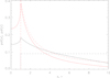 |
Fig. A.1. Probability density functions of radial (dashed) and x (solid) coordinates for different spherical and Cartesian grids. In this example, two spherical grids are given in 2D as input to our 3D code, with uniformly (black) or logarithmically (red) distributed r-coordinates, and a uniformly distributed polar angle. The corresponding distributions of x-coordinates are calculated within our grid construction procedure (see text). Large values of the probability density functions correspond to a high resolution of x and r-coordinates. |
Since the final number of core and non-core points depends on the slope of the probability density of the radial grid, yielding in worst cases a much larger number of core points than non-core points, and because the total number of used points is memory-limited, we define two input parameters Ncore and Nnon − core to keep control on the final grid. For all test calculations (including those presented in Sect. 4.2), the best solution has always been found for a number of Ncore/Nnon − core ∈ [0.25, 0.5]. An explicit choice of Ncore and Nnon − core corresponds to a re-normalization of the probability density function in the regimes x, z ∈ [0, R*] and x, z ∈ [R*, Rmax], where Rmax defines the border of the computational domain. We note that the same procedure can be used for an input grid given in Cartesian coordinates, with the probability density function of the input-grid coordinates derived directly from the corresponding (discrete) distribution.
Appendix B: 1D Bézier interpolation
In this section, we discuss an interpolation technique using quadratic Bézier curves (e.g. Auer 2003; Schwarz 1997). Such curves are generally constructed from three given points b0, b1, b2 (see Fig. B.1), and have the following useful properties:
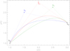 |
Fig. B.1. Bézier curves (solid lines) for three given points b0, b1, b2. The blue, red, and green lines represent the resulting curves for different control points b1. The straight connections of the control points with the data points are indicated by the dotted lines. |
-
(i)
The boundary points, b0 and b2 are reproduced exactly by the Bézier curve.
-
(ii)
The straight connections (b1−b0) and (b2−b1) define the tangent lines of the curve at b0 and b2, respectively.
-
(iii)
Any point on the Bézier curve is located in the convex hull of b0, b1, b2.
In a 2D plane described by coordinates x and y, the quadratic Bézier curve is parameterized as:
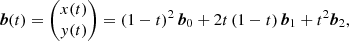 (B.1)
(B.1)
with t ∈ [0, 1], and b0 = (x0, y0), b1 = (x1, y1), b2 = (x2, y2). With Eq. (B.1), the properties (i)–(iii) can be exploited to construct a monotonic interpolation scheme by identifying b0,b2 with two given data points (x0, f0), (x2, f2), and defining b1 as a free (and tunable) parameter. Thus, b1 is commonly named control point, and is “only” required to set the slope of the Bézier curve. To reproduce the underlying function best, and to preserve monotonicity of the resulting curve, the control point should be chosen with care.
In the following, we present a Bézier-interpolation technique for an interval x ∈ [xi − 1, xi], given three data points, (xi − 1, fi − 1), (xi, fi), (xi + 1, fi + 1). The interpolation formulas corresponding to the interval x ∈ [xi, xi + 1] are given in Appendix B.2.
B.1. Interval [xi − 1, xi]
A quadratic Bézier curve in the interval [xi − 1, xi] is given from Eq. (B.1):
 (B.2)
(B.2)
with (xc, fc) the control point. The abscissa of the control point, xc, can be chosen arbitrarily (at least in principal). To obtain a second-order interpolation scheme, however, xc needs to be located at the centre of the data-point’s abscissae9, and is therefore set to xc = (xi − 1 + xi)/2. Then, the quadratic Bézier interpolation scheme is given by:
 (B.3)
(B.3)
where t has been determined from the definition of xc and Eq. (B.2). Since the straight connection of the control point (xc, fc) with the data point (xi, fi) defines the tangent line of the Bézier curve at this data point, fc is calculated as
with Δxi = xi − xi − 1. The unknown derivative at xi needs to be approximated. Using also the information from the next data point, (xi + 1, fi + 1), and assigning a weight ω to the forward and backward derivatives (obtained from finite differences), we find
 (B.4)
(B.4)
with Δxi + 1 = xi + 1 − xi. With a proper choice of ω, we can adjust the Bézier curve to our needs by shifting the control point up or down. For instance, setting ω = Δxi + 1/(Δxi + Δxi + 1) results in the unique parabola connecting the three given data points, while ω = 1 would yield the linear interpolation. To avoid overshoots and negative function values, we demand that the Bézier curve shall be monotonic in the interval [xi − 1, xi]. Noting that monotonicity is obtained when the control point is located in the interval fc ∈ [fi − 1, fi], corresponding ω-values should lie in between the following limits:
![Mathematical equation: $$ \begin{aligned} \omega _{{i-1}}^{[{i-1},{i}]}&:= \omega \left(f_{\mathrm{c}}^{[{i-1},{i}]}=f_{i-1}\right) = 1 + \dfrac{1}{1-\frac{f_{i+1}-f_{i}}{f_{i}-f_{i-1}}\frac{\Delta x_{i}}{\Delta x_{i+1}}} \end{aligned} $$](/articles/aa/full_html/2020/01/aa36584-19/aa36584-19-eq113.gif) (B.5)
(B.5)
![Mathematical equation: $$ \begin{aligned} \omega _{{i}}^{[{i-1},{i}]}&:= \omega \left(f_{\mathrm{c}}^{[{i-1},{i}]}=f_{i}\right) = \dfrac{1}{1-\frac{f_{i}-f_{i-1}}{f_{i+1}-f_{i}}\frac{\Delta x_{i+1}}{\Delta x_{i}}}, \end{aligned} $$](/articles/aa/full_html/2020/01/aa36584-19/aa36584-19-eq114.gif) (B.6)
(B.6)
where the superscript [i − 1, i] denotes that ω corresponds to the interpolation scheme in the left interval, [xi − 1, xi]. In the final implementation, we avoid the division by zero if fi = fi − 1 or fi = fi + 1, of course. Our standard interpolation is then performed as follows. At first, we calculate ω such that we obtain the unique parabola connecting all three data points. Secondly, if ω lies outside the allowed limits from Eq. (B.5) and (B.6), we adjust ω to yield monotonic interpolations. In Fig. B.2, we display the monotonic Bézier curve resulting from a ω-parameter calculated by means of Eq. (B.5), together with linear and quadratic interpolations (the latter connecting the three data points). Since monotonicity is always obtained for ω ∈ [ωi − 1, ωi], we can define even stricter limits in order to avoid oscillations during the iteration scheme, by setting ω = 1 to obtain purely linear interpolations, for instance (see Sect. 3.6).
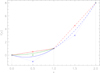 |
Fig. B.2. Different interpolation techniques for a set of three data points at x-coordinates indicated by the dotted vertical lines. The solid and dashed lines correspond to the interpolation in the different intervals [xi − 1, xi] and [xi, xi + 1], respectively. Linear interpolations, quadratic interpolations (connecting all three data points), and a monotonic Bézier curve (with ω calculated from Eq. (B.5) in the interval [xi − 1, xi]) are indicated in red, blue, and green. Since the quadratic interpolation is already monotonic in the interval [xi, xi + 1], the monotonic Bézier curve coincides with the dashed, blue line. Control points are indicated with coloured asterisks. |
To calculate the elements of the (approximate) Λ-matrix, the interpolation coefficients are required. Combining Eqs. (B.3) and (B.4) then gives:
![Mathematical equation: $$ \begin{aligned} f\bigl (x\in [x_{i-1},x_{i}]\bigr ) = \tilde{a}^{[{i-1},{i}]}f_{i-1}+ \tilde{b}^{[{i-1},{i}]}f_{i}+ \tilde{c}^{[{i-1},{i}]}f_{i+1}, \end{aligned} $$](/articles/aa/full_html/2020/01/aa36584-19/aa36584-19-eq115.gif) (B.7)
(B.7)
with
![Mathematical equation: $$ \begin{aligned} \tilde{a}^{[{i-1},{i}]} =&1 + (\omega -2)\dfrac{x-x_{i-1}}{x_{i}-x_{i-1}} + (1-\omega )\Biggl (\dfrac{x-x_{i-1}}{x_{i}-x_{i-1}}\Biggr )^2 \end{aligned} $$](/articles/aa/full_html/2020/01/aa36584-19/aa36584-19-eq116.gif) (B.8)
(B.8)
![Mathematical equation: $$ \begin{aligned} \nonumber \tilde{b}^{[{i-1},{i}]} =&\dfrac{(1-\omega )\Delta x_{i}+(2-\omega )\Delta x_{i+1}}{\Delta x_{i+1}}\dfrac{x-x_{i-1}}{x_{i}-x_{i-1}} \\&+ (\omega -1) \dfrac{\Delta x_{i}+\Delta x_{i+1}}{\Delta x_{i+1}}\Biggl ( \dfrac{x-x_{i-1}}{x_{i}-x_{i-1}} \Biggr )^2 \end{aligned} $$](/articles/aa/full_html/2020/01/aa36584-19/aa36584-19-eq117.gif) (B.9)
(B.9)
![Mathematical equation: $$ \begin{aligned} \nonumber \tilde{c}^{[{i-1},{i}]} =&\dfrac{(\omega -1)\Delta x_{i}}{\Delta x_{i+1}}\dfrac{x-x_{i-1}}{x_{i}-x_{i-1}} \\&-\dfrac{(\omega -1)\Delta x_{i}}{\Delta x_{i+1}}\Biggl (\dfrac{x-x_{i-1}}{x_{i}-x_{i-1}}\Biggr )^2\cdot \end{aligned} $$](/articles/aa/full_html/2020/01/aa36584-19/aa36584-19-eq118.gif) (B.10)
(B.10)
B.2. Interval [xi, xi + 1]
The interpolation formula for the right interval [xi, xi + 1] uses the same data points as above. Since the value of the control point needs to be calculated at a different x-coordinate, xc = (xi + 1 + xi)/2, we cannot simply substitute indices. Using
 (B.11)
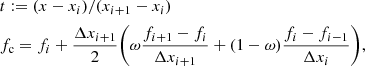 (B.12)
we obtain for this interval:
![Mathematical equation: $$ \begin{aligned} f(x\in [x_{i},x_{i+1}]) = \tilde{a}^{[{i},{i+1}]}f_{i-1}+ \tilde{b}^{[{i},{i+1}]}f_{i}+ \tilde{c}^{[{i},{i+1}]}f_{i+1}\,, \end{aligned} $$](/articles/aa/full_html/2020/01/aa36584-19/aa36584-19-eq121.gif) (B.13)
(B.13)
with
![Mathematical equation: $$ \begin{aligned} \tilde{a}^{[{i},{i+1}]} =&\dfrac{(\omega -1)\Delta x_{i+1}}{\Delta x_{i}}\dfrac{x-x_{i}}{x_{i+1}-x_{i}}\nonumber \\&- \dfrac{(\omega -1)\Delta x_{i+1}}{\Delta x_{i}}\Biggl (\dfrac{x-x_{i}}{x_{i+1}-x_{i}}\Biggr )^2 \end{aligned} $$](/articles/aa/full_html/2020/01/aa36584-19/aa36584-19-eq122.gif) (B.14)
(B.14)
![Mathematical equation: $$ \begin{aligned} {{\tilde b}^{[i,i + 1]}} = &\ 1 - \frac{{\omega \Delta {x_i} + (\omega - 1)\Delta {x_{i + 1}}}}{{\Delta {x_i}}}\frac{{x - {x_i}}}{{{x_{i + 1}} - {x_i}}}\nonumber\\& + (\omega - 1)\frac{{\Delta {x_i} + \Delta {x_{i + 1}}}}{{\Delta {x_i}}}{(\frac{{x - {x_i}}}{{{x_{i + 1}} - {x_i}}})^2} \end{aligned} $$](/articles/aa/full_html/2020/01/aa36584-19/aa36584-19-eq123.gif) (B.15)
(B.15)
![Mathematical equation: $$ \begin{aligned} \tilde{c}^{[{i},{i+1}]} =&\omega \dfrac{x-x_{i}}{x_{i+1}-x_{i}} + (1-\omega )\Biggl (\dfrac{x-x_{i}}{x_{i+1}-x_{i}}\Biggr )^2, \end{aligned} $$](/articles/aa/full_html/2020/01/aa36584-19/aa36584-19-eq124.gif) (B.16)
(B.16)
and
![Mathematical equation: $$ \begin{aligned} \omega _{{i}}^{[{i},{i+1}]}&:= \omega (f_{\mathrm{c}}^{[{i},{i+1}]}=f_{i}) = \dfrac{1}{1-\frac{f_{i+1}-f_{i}}{f_{i}-f_{i-1}}\frac{\Delta x_{i}}{\Delta x_{i+1}}} \end{aligned} $$](/articles/aa/full_html/2020/01/aa36584-19/aa36584-19-eq125.gif) (B.17)
(B.17)
![Mathematical equation: $$ \begin{aligned} \omega _{{i+1}}^{[{i},{i+1}]}&:= \omega (f_{\mathrm{c}}^{[{i},{i+1}]}=f_{i+1}) = 1 + \dfrac{1}{1-\frac{f_{i}-f_{i-1}}{f_{i+1}-f_{i}}\frac{\Delta x_{i+1}}{\Delta x_{i}}}\cdot \end{aligned} $$](/articles/aa/full_html/2020/01/aa36584-19/aa36584-19-eq126.gif) (B.18)
(B.18)
The corresponding Bézier curves for different ω-parameters (ω = 1 for linear and ω = Δxi/(Δxi + Δxi + 1) for continuous quadratic interpolations) are also shown in Fig. B.2. We note that the Bézier interpolation gives a continuous function in the complete interval [xi − 1, xi + 1] only for those ω-values that define the parabola connecting all three data points.
Appendix C: 2D Bézier interpolation
To interpolate upwind and downwind quantities, a 2D interpolation scheme is required. Figure C.1 displays the geometry for a 2D rectangular area, with grid points indicated by the black dots. With this setup, we perform a 2D Bézier interpolation by applying three 1D Bézier interpolations along the x-axis on each y-level at (j − 1), (j), (j + 1), followed by another 1D Bézier interpolation along y at the desired x-coordinate. Within the cyan shaded interval, we obtain with the 1D Bézier interpolation given by Eqs. (B.13)–(B.16):
 (C.1)
(C.1)
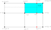 |
Fig. C.1. 2D interpolation for upwind or downwind quantities required in the cyan shaded area. The 2D Bézier interpolation consists of three 1D interpolations to obtain the values at the desired x-coordinate (indicated by red dots), followed by a 1D interpolation along the y-coordinate using the obtained values at the red dots. |
where the subscripts of the interpolation coefficients indicate the coordinate used for each 1D interpolation. We note that all upwind and downwind interpolations are performed in the upper right interval of a given surface, in order to obtain a simple representation of the Λ-matrix elements.
Appendix D: ALO coefficients
In this section, we derive the Λ-matrix coefficients used to construct the approximate Λ-operator. We note that the obtained matrix elements can also be used for any other (2nd or lower order) interpolation scheme using the same geometry, with different interpolation coefficients though.
For a source function set to unity at grid point (ijk) and zero everywhere else, we consider all 27 points ranging from (i − α, j − β, k − γ) to (i + α, j + β, k + γ). The corresponding matrix coefficients are derived from Eq. (29), using the discretized equation of radiative transfer, Eqs. (12)/(20), with upwind and downwind interpolations defined by Eqs. (22) and (23). We further consider only the ΛΩν-operator, since the integration over frequency and/or solid angle is straightforward. Each Λ-matrix element then corresponds to the intensity (resulting from Sijk = 1) at a considered grid point p (not necessarily identical to (ijk)), and consists of an emission term (defined by the interpolated source functions and optical-depth steps at the corresponding upwind, current, and downwind points), and the irradiation from the upwind point (defined by the upwind intensity and upwind optical-depth step). The upper and lower panel of Fig. D.1 show an example in 2D considering the points (i − α, j − β) and (i, j − β) for a source function Sij = 1.
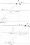 |
Fig. D.1. 2D example for calculating the ΛΩ, ν-matrix elements at a grid point (i − α, j − β) (upper panel) and (i, j − β) (lower panel). The matrix elements correspond to the intensity at the considered grid points calculated for a source function Sij = 1 and zero everywhere else. For such a configuration, the downwind source function is interpolated from grid points indicated with the green dots, while the upwind source function and upwind intensity are obtained from the red dots (for simplicity we here assume linear interpolations for determining upwind and downwind quantities). We emphasize that the upwind intensity vanishes only when considering the grid point (i − α, j − β). |
In the following, we sketch the derivation of the (3D) matrix element for the first neighbour, and only present the solution for the remaining ones. To save space, we skip the indices Ω, ν. The m, nth Λ-element is written as  , with matrix indices n, m calculated from Eq. (30). While n corresponds to the 3D indices of the local grid point (Sijk = Sn = 1), m represents the neighbouring point, (i − α, j − β, k − γ). Applying Eq. (29) to the specific intensity at point m, we obtain:
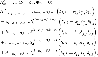
with boundary contribution ΦB, nth unit vector en, and  ,
,  ,
,  the Kronecker-δ for all possible
  ,
,  , and
, and  coordinates, respectively. Su and Sd are the upwind and downwind source functions corresponding to a considered short characteristic at grid point p ↔ (i − α, j − β, k − γ), Sp is the source function at the grid point10, Iu is the upwind intensity, and a, b, c, d are the integration coefficients for this particular short characteristic. All upwind and downwind quantities are to be interpolated from neighbouring grid points. We use the notation w,
  ,
,  , to identify different interpolation coefficients corresponding to the upwind source function, upwind intensity, and downwind source function, respectively. Using Eqs. (22) and (23) to interpolate upwind and downwind quantities, we find:
![Mathematical equation: $$ \begin{aligned} \Lambda _{{i-\alpha ,j-\beta ,k-\gamma }}^{{ijk}} =&a_{{i-\alpha ,j-\beta ,k-\gamma }}\times \bigl [ w_{\rm A} S_{{i-3\alpha ,j-2\beta ,k-3\gamma }}\\&+ w_{\rm B} S_{{i-2\alpha ,j-2\beta ,k-3\gamma }} +w_{\rm C} S_{{i-\alpha ,j-2\beta ,k-3\gamma }}\\&+ w_{\rm D} S_{{i-3\alpha ,j-2\beta ,k-2\gamma }} +w_{\rm E} S_{{i-2\alpha ,j-2\beta ,k-2\gamma }}\\&+ w_{\rm F} S_{{i-\alpha ,j-2\beta ,k-2\gamma }} +w_{\rm G} S_{{i-3\alpha ,j-2\beta ,k-\gamma }}\\&+ w_{\rm H} S_{{i-2\alpha ,j-2\beta ,k-\gamma }} +w_{\rm I} S_{{i-\alpha ,j-2\beta ,k-\gamma }}\\&+ w_{\rm J} S_{{i-3\alpha ,j-3\beta ,k-2\gamma }} +w_{\rm K} S_{{i-2\alpha ,j-3\beta ,k-2\gamma }}\\&+ w_{\rm L} S_{{i-\alpha ,j-3\beta ,k-2\gamma }} +w_{\rm M} S_{{i-3\alpha ,j-\beta ,k-2\gamma }}\\&+ w_{\rm N} S_{{i-2\alpha ,j-\beta ,k-2\gamma }} +w_{\rm O} S_{{i-\alpha ,j-\beta ,k-2\gamma }}\\&+ w_{\rm P} S_{{i-2\alpha ,j-3\beta ,k-3\gamma }} +w_{\rm Q} S_{{i-2\alpha ,j-\beta ,k-3\gamma }}\\&+ w_{\rm R} S_{{i-2\alpha ,j-3\beta ,k-\gamma }} +w_{\rm S} S_{{i-2\alpha ,j-\beta ,k-\gamma }}\\&+ w_{{i-\alpha ,j-\beta ,k-\gamma }} S_{{ i-\alpha ,j-\beta ,k-\gamma }} \bigr ]\\&+ b_{{i-\alpha ,j-\beta ,k-\gamma }} S_{{ i-\alpha , j-\beta ,k-\gamma }}\\&+ c_{{i-\alpha ,j-\beta ,k-\gamma }} \times \bigl [ \tilde{w}_{\rm A} S_{{ i-2\alpha ,j,k-2\gamma }}\\&+ \tilde{w}_{\rm B} S_{{ i-\alpha ,j,k-2\gamma }} +\tilde{w}_{\rm C} S_{{ i,j,k-2\gamma }}\\&+ \tilde{w}_{\rm D} S_{{ i-2\alpha ,j,k-\gamma }} +\tilde{w}_{\rm E} S_{{ i-\alpha ,j,k-\gamma }}\\&+ \tilde{w}_{\rm F} S_{{ i,j,k-\gamma }} +\tilde{w}_{\rm G} S_{{ i-2\alpha ,j,k}}\\&+ \tilde{w}_{\rm H} S_{{ i-\alpha ,j,k}} +\tilde{w}_{\rm I} S_{{ i,j,k}}\\&+ \tilde{w}_{\rm J} S_{{ i-2\alpha ,j-2\beta ,k}} +\tilde{w}_{\rm K} S_{{ i-\alpha ,j-2\beta ,k}}\\&+ \tilde{w}_{\rm L} S_{{ i,j-2\beta ,k}} +\tilde{w}_{\rm M} S_{{ i-2\alpha ,j-\beta ,k}}\\&+ \tilde{w}_{\rm N} S_{{ i-\alpha ,j-\beta ,k}} +\tilde{w}_{\rm O} S_{{ i,j-\beta ,k}}\\&+ \tilde{w}_{\rm P} S_{{ i,j-2\beta ,k-2\gamma }} +\tilde{w}_{\rm Q} S_{{ i,j-\beta ,k-2\gamma }}\\&+ \tilde{w}_{\rm R} S_{{ i,j-2\beta ,k-\gamma }} +\tilde{w}_{\rm S} S_{{ i,j-\beta ,k-\gamma }} \bigr ]\\&+ d_{{i-\alpha ,j-\beta ,k-\gamma }} \bigl [\hat{w}_{\rm A} I_{{i-3\alpha ,j-2\beta ,k-3\gamma }} (S_{{ijk}}=1) + \ldots \\&+ \hat{w}_{\rm S} I_{{i-2\alpha , j-\beta , k-\gamma }} (S_{{ ijk}} = 1)\bigr ], \end{aligned} $$](/articles/aa/full_html/2020/01/aa36584-19/aa36584-19-eq138.gif)
with the upwind intensity interpolated from the same points as the upwind source function, and a compact notation for the interpolation coefficients (with skipped superscripts). Since only Sijk = 1 (and zero everywhere else), and because the upwind intensity vanishes (for this particular grid point, see Fig. D.1 for an example in 2D), we finally obtain:
 (D.1)
(D.1)
The matrix element for a point (i − α, j − β, k − γ) with a non-vanishing source function at point (ijk) is thus solely given by the integration coefficient ci − α, j − β, k − γ from the discretized equation of radiative transfer multiplied with the interpolation coefficient for the downwind source function of point I (corresponding to grid point (ijk), see Fig. 1). The other neighbours are obtained analogously, without vanishing incident intensities, however. Accounting also for the interpolation of upwind source functions and intensities when necessary, we find:
 (D.2)
(D.2)
 (D.3)
(D.3)
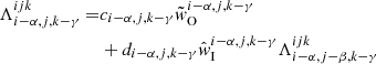 (D.4)
(D.4)
![Mathematical equation: $$ \begin{aligned} \Lambda _{{i,j,k-\gamma }}^{{ijk}} =&c_{{i,j,k-\gamma }}\tilde{w}_{\rm N}^{{i,j,k-\gamma }} + d_{{i,j,k-\gamma }} \times \Bigl [ \hat{w}_{\rm H}^{{i,j,k-\gamma }} \Lambda _{{i-\alpha ,j-\beta ,k-\gamma }}^{{ijk}}\nonumber \\&+ \hat{w}_{\rm I}^{{i,j,k-\gamma }} \Lambda _{{i,j-\beta ,k-\gamma }}^{{ijk}} + \hat{w}_{\rm S}^{{i,j,k-\gamma }} \Lambda _{{i-\alpha ,j,k-\gamma }}^{{ijk}} \Bigr ] \end{aligned} $$](/articles/aa/full_html/2020/01/aa36584-19/aa36584-19-eq143.gif) (D.5)
(D.5)
![Mathematical equation: $$ \begin{aligned} \Lambda _{{i+\alpha ,j,k-\gamma }}^{{ijk}} =&c_{{i+\alpha ,j,k-\gamma }}\tilde{w}_{\rm M}^{{i+\alpha ,j,k-\gamma }} + d_{{i+\alpha ,j,k-\gamma }}\nonumber \\&\times \Bigl [ \hat{w}_{\rm D}^{{i+\alpha ,j,k-\gamma }} \Lambda _{{i-\alpha ,j-\beta ,k-\gamma }}^{{ijk}} + \hat{w}_{\rm H}^{{i+\alpha ,j,k-\gamma }} \Lambda _{{i,j-\beta ,k-\gamma }}^{{ijk}}\nonumber \\&+ \hat{w}_{\rm I}^{{i+\alpha ,j,k-\gamma }} \Lambda _{{i+\alpha ,j-\beta ,k-\gamma }}^{{ijk}} + \hat{w}_{\rm S}^{{i+\alpha ,j,k-\gamma }} \Lambda _{{i,j,k-\gamma }}^{{ijk}} \Bigr ] \end{aligned} $$](/articles/aa/full_html/2020/01/aa36584-19/aa36584-19-eq144.gif) (D.6)
(D.6)
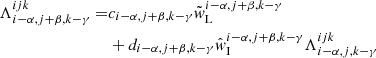 (D.7)
(D.7)
![Mathematical equation: $$ \begin{aligned} \Lambda _{{i,j+\beta ,k-\gamma }}^{{ijk}} =&c_{{i,j+\beta ,k-\gamma }}\tilde{w}_{\rm K}^{{i,j+\beta ,k-\gamma }} + d_{{i,j+\beta ,k-\gamma }}\nonumber \\&\times \Bigl [ \hat{w}_{\rm R}^{{i,j+\beta ,k-\gamma }}\Lambda _{{i-\alpha ,j-\beta ,k-\gamma }}^{{ijk}}+ \hat{w}_{\rm H}^{{i,j+\beta ,k-\gamma }}\Lambda _{{i-\alpha ,j,k-\gamma }}^{{ijk}}\nonumber \\&+ \hat{w}_{\rm I}^{{i,j+\beta ,k-\gamma }}\Lambda _{{i,j,k-\gamma }}^{{ijk}}+ \hat{w}_{\rm S}^{{i,j+\beta ,k-\gamma }}\Lambda _{{i-\alpha ,j+\beta ,k-\gamma }}^{{ijk}} \Bigr ] \end{aligned} $$](/articles/aa/full_html/2020/01/aa36584-19/aa36584-19-eq146.gif) (D.8)
(D.8)
![Mathematical equation: $$ \begin{aligned} \Lambda _{{i+\alpha ,j+\beta ,k-\gamma }}^{{ijk}} =&c_{{i+\alpha ,j+\beta ,k-\gamma }}\tilde{w}_{\rm J}^{{i+\alpha ,j+\beta ,k-\gamma }} + d_{{i+\alpha ,j+\beta ,k-\gamma }}\nonumber \\&\times \Bigl [ \hat{w}_{\rm R}^{{i+\alpha ,j+\beta ,k-\gamma }}\Lambda _{{i,j-\beta ,k-\gamma }}^{{ijk}}+ \hat{w}_{\rm G}^{{i+\alpha ,j+\beta ,k-\gamma }}\Lambda _{{i-\alpha ,j,k-\gamma }}^{{ijk}}\nonumber \\&+ \hat{w}_{\rm H}^{{i+\alpha ,j+\beta ,k-\gamma }}\Lambda _{{i,j,k-\gamma }}^{{ijk}}+ \hat{w}_{\rm I}^{{i+\alpha ,j+\beta ,k-\gamma }}\Lambda _{{i+\alpha ,j,k-\gamma }}^{{ijk}}\nonumber \\&+ \hat{w}_{\rm S}^{{i+\alpha ,j+\beta ,k-\gamma }}\Lambda _{{i,j+\beta ,k-\gamma }}^{{ijk}}\Bigr ] \end{aligned} $$](/articles/aa/full_html/2020/01/aa36584-19/aa36584-19-eq147.gif) (D.9)
(D.9)
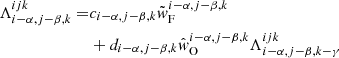 (D.10)
![Mathematical equation: $$ \begin{aligned} \Lambda _{{i,j-\beta ,k}}^{{ijk}} =&c_{{i,j-\beta ,k}}\tilde{w}_{\rm E}^{{i,j-\beta ,k}} + d_{{i,j-\beta ,k}} \times \Bigl [\hat{w}_{\rm N}^{{i,j-\beta ,k}}\Lambda _{{i-\alpha ,j-\beta ,k-\gamma }}^{{ijk}}\nonumber \\&+ \hat{w}_{\rm O}^{{i,j-\beta ,k}}\Lambda _{{i,j-\beta ,k-\gamma }}^{{ijk}} + \hat{w}_{\rm S}^{{i,j-\beta ,k}}\Lambda _{{i-\alpha ,j-\beta ,k}}^{{ijk}} \Bigr ] \end{aligned} $$](/articles/aa/full_html/2020/01/aa36584-19/aa36584-19-eq149.gif) (D.11)
(D.11)
![Mathematical equation: $$ \begin{aligned} \Lambda _{{i+\alpha ,j-\beta ,k}}^{{ijk}} =&c_{{i+\alpha ,j-\beta ,k}}\tilde{w}_{\rm D}^{{i+\alpha ,j-\beta ,k}} + d_{{i+\alpha ,j-\beta ,k}}\nonumber \\&\times \Bigl [\hat{w}_{\rm M}^{{i+\alpha ,j-\beta ,k}}\Lambda _{{i-\alpha ,j-\beta ,k-\gamma }}^{{ijk}}+ \hat{w}_{\rm N}^{{i+\alpha ,j-\beta ,k}}\Lambda _{{i,j-\beta ,k-\gamma }}^{{ijk}}\nonumber \\&+ \hat{w}_{\rm O}^{{i+\alpha ,j-\beta ,k}}\Lambda _{{i+\alpha ,j-\beta ,k-\gamma }}^{{ijk}}+ \hat{w}_{\rm S}^{{i+\alpha ,j-\beta ,k}}\Lambda _{{i,j-\beta ,k}}^{{ijk}} \Bigr ] \end{aligned} $$](/articles/aa/full_html/2020/01/aa36584-19/aa36584-19-eq150.gif) (D.12)
(D.12)
![Mathematical equation: $$ \begin{aligned} \Lambda _{{i-\alpha ,j,k}}^{{ijk}} =&c_{{i-\alpha ,j,k}}\tilde{w}_{\rm S}^{{i-\alpha ,j,k}} + d_{{i-\alpha ,j,k}} \times \Bigl [\hat{w}_{\rm F}^{{i-\alpha ,j,k}} \Lambda _{{i-\alpha ,j-\beta ,k-\gamma }}^{{ijk}}\nonumber \\&+ \hat{w}_{\rm O}^{{i-\alpha ,j,k}} \Lambda _{{i-\alpha ,j,k-\gamma }}^{{ijk}} + \hat{w}_{\rm I}^{{i-\alpha ,j,k}} \Lambda _{{i-\alpha ,j-\beta ,k}}^{{ijk}} \Bigr ] \end{aligned} $$](/articles/aa/full_html/2020/01/aa36584-19/aa36584-19-eq151.gif) (D.13)
(D.13)
![Mathematical equation: $$ \begin{aligned} \Lambda _{{ijk}}^{{ijk}} =&a_{{ijk}}w_{{ijk}} + b_{{ijk}} + d_{{ijk}}\nonumber \\&\times \Bigl [ \hat{w}_{\rm E}^{{ijk}} \Lambda _{{i-\alpha ,j-\beta ,k-\gamma }}^{{ijk}} + \hat{w}_{\rm F}^{{ijk}} \Lambda _{{i,j-\beta ,k-\gamma }}^{{ijk}}\nonumber \\&+ \hat{w}_{\rm N}^{{ijk}} \Lambda _{{i-\alpha ,j,k-\gamma }}^{{ijk}} + \hat{w}_{\rm O}^{{ijk}} \Lambda _{{i,j,k-\gamma }}^{{ijk}} + \hat{w}_{\rm H}^{{ijk}} \Lambda _{{i-\alpha ,j-\beta ,k}}^{{ijk}}\nonumber \\&+ \hat{w}_{\rm I}^{{ijk}} \Lambda _{{i,j-\beta ,k}}^{{ijk}} + \hat{w}_{\rm S}^{{ijk}} \Lambda _{{i-\alpha ,j,k}}^{{ijk}} \Bigr ] \end{aligned} $$](/articles/aa/full_html/2020/01/aa36584-19/aa36584-19-eq152.gif) (D.14)
(D.14)
![Mathematical equation: $$ \begin{aligned} \Lambda _{{i+\alpha ,j,k}}^{{ijk}} =&a_{{i+\alpha ,j,k}}w_{\rm S}^{{i+\alpha ,j,k}} + d_{{i+\alpha ,j,k}}\nonumber \\& \times \Bigl [ \hat{w}_{\rm D}^{{i+\alpha ,j,k}} \Lambda _{{i-\alpha ,j-\beta ,k-\gamma }}^{{ijk}} + \hat{w}_{\rm E}^{{i+\alpha ,j,k}} \Lambda _{{i,j-\beta ,k-\gamma }}^{{ijk}}\nonumber \\&+ \hat{w}_{\rm F}^{{i+\alpha ,j,k}} \Lambda _{{i+\alpha ,j-\beta ,k-\gamma }}^{{ijk}} + \hat{w}_{\rm M}^{{i+\alpha ,j,k}} \Lambda _{{i-\alpha ,j,k-\gamma }}^{{ijk}}\nonumber \\&+ \hat{w}_{\rm N}^{{i+\alpha ,j,k}} \Lambda _{{i,j,k-\gamma }}^{{ijk}} + \hat{w}_{\rm O}^{{i+\alpha ,j,k}} \Lambda _{{i+\alpha ,j,k-\gamma }}^{{ijk}}\nonumber \\&+ \hat{w}_{\rm G}^{{i+\alpha ,j,k}} \Lambda _{{i-\alpha ,j-\beta ,k}}^{{ijk}} + \hat{w}_{\rm H}^{{i+\alpha ,j,k}} \Lambda _{{i,j-\beta ,k}}^{{ijk}}\nonumber \\&+ \hat{w}_{\rm I}^{{i+\alpha ,j,k}} \Lambda _{{i+\alpha ,j-\beta ,k}}^{{ijk}} + \hat{w}_{\rm S}^{{i+\alpha ,j,k}} \Lambda _{{ijk}}^{{ijk}} \Bigr ] \end{aligned} $$](/articles/aa/full_html/2020/01/aa36584-19/aa36584-19-eq153.gif) (D.15)
(D.15)
![Mathematical equation: $$ \begin{aligned} \Lambda _{{i-\alpha ,j+\beta ,k}}^{{ijk}} =&c_{{i-\alpha ,j+\beta ,k}}\tilde{w}_{\rm R}^{{i-\alpha ,j+\beta ,k}} + d_{{i-\alpha ,j+\beta ,k}}\nonumber \\&\times \Bigl [ \hat{w}_{\rm L}^{{i-\alpha ,j+\beta ,k}} \Lambda _{{i-\alpha ,j-\beta ,k-\gamma }}^{{ijk}} + \hat{w}_{\rm F}^{{i-\alpha ,j+\beta ,k}} \Lambda _{{i-\alpha ,j,k-\gamma }}^{{ijk}}\nonumber \\&+ \hat{w}_{\rm O}^{{i-\alpha ,j+\beta ,k}} \Lambda _{{i-\alpha ,j+\beta ,k-\gamma }}^{{ijk}} + \hat{w}_{\rm I}^{{i-\alpha ,j+\beta ,k}} \Lambda _{{i-\alpha ,j,k}}^{{ijk}} \Bigr ] \end{aligned} $$](/articles/aa/full_html/2020/01/aa36584-19/aa36584-19-eq154.gif) (D.16)
(D.16)
![Mathematical equation: $$ \begin{aligned} \Lambda _{{i,j+\beta ,k}}^{{ijk}} =&a_{{i,j+\beta ,k}}w_{\rm I}^{{i,j+\beta ,k}} + d_{{i,j+\beta ,k}}\nonumber \\& \times \Bigl [ \hat{w}_{\rm E}^{{i,j+\beta ,k}} \Lambda _{{i-\alpha ,j,k-\gamma }}^{{ijk}} + \hat{w}_{\rm F}^{{i,j+\beta ,k}} \Lambda _{{i,j,k-\gamma }}^{{ijk}}\nonumber \\&+ \hat{w}_{\rm H}^{{i,j+\beta ,k}} \Lambda _{{i-\alpha ,j,k}}^{{ijk}} + \hat{w}_{\rm I}^{{i,j+\beta ,k}} \Lambda _{{ijk}}^{{ijk}}\nonumber \\&+ \hat{w}_{\rm K}^{{i,j+\beta ,k}} \Lambda _{{i-\alpha ,j-\beta ,k-\gamma }}^{{ijk}} + \hat{w}_{\rm L}^{{i,j+\beta ,k}} \Lambda _{{i,j-\beta ,k-\gamma }}^{{ijk}}\nonumber \\&+ \hat{w}_{\rm N}^{{i,j+\beta ,k}} \Lambda _{{i-\alpha ,j+\beta ,k-\gamma }}^{{ijk}} + \hat{w}_{\rm O}^{{i,j+\beta ,k}} \Lambda _{{i,j+\beta ,k-\gamma }}^{{ijk}}\nonumber \\&+ \hat{w}_{\rm R}^{{i,j+\beta ,k}} \Lambda _{{i-\alpha ,j-\beta ,k}}^{{ijk}} + \hat{w}_{\rm S}^{{i,j+\beta ,k}} \Lambda _{{i-\alpha ,j+\beta ,k}}^{{ijk}} \Bigr ] \end{aligned} $$](/articles/aa/full_html/2020/01/aa36584-19/aa36584-19-eq155.gif) (D.17)
(D.17)
![Mathematical equation: $$ \begin{aligned} \Lambda _{{i+\alpha ,j+\beta ,k}}^{{ijk}} =&a_{{i+\alpha ,j+\beta ,k}}w_{\rm H}^{{i+\alpha ,j+\beta ,k}} + d_{{i+\alpha ,j+\beta ,k}}\nonumber \\&\times \Bigl [ \hat{w}_{\rm D}^{{i+\alpha ,j+\beta ,k}} \Lambda _{{i-\alpha ,j,k-\gamma }}^{{ijk}} + \hat{w}_{\rm E}^{{i+\alpha ,j+\beta ,k}} \Lambda _{{i,j,k-\gamma }}^{{ijk}}\nonumber \\&+ \hat{w}_{\rm F}^{{i+\alpha ,j+\beta ,k}} \Lambda _{{i+\alpha ,j,k-\gamma }}^{{ijk}} + \hat{w}_{\rm G}^{{i+\alpha ,j+\beta ,k}} \Lambda _{{i-\alpha ,j,k}}^{{ijk}}\nonumber \\&+ \hat{w}_{\rm H}^{{i+\alpha ,j+\beta ,k}} \Lambda _{{ijk}}^{{ijk}} + \hat{w}_{\rm I}^{{i+\alpha ,j+\beta ,k}} \Lambda _{{i+\alpha ,j,k}}^{{ijk}}\nonumber \\&+\hat{w}_{\rm J}^{{i+\alpha ,j+\beta ,k}} \Lambda _{{i-\alpha ,j-\beta ,k-\gamma }}^{{ijk}} + \hat{w}_{\rm K}^{{i+\alpha ,j+\beta ,k}} \Lambda _{{i,j-\beta ,k-\gamma }}^{{ijk}}\nonumber \\&+ \hat{w}_{\rm L}^{{i+\alpha ,j+\beta ,k}} \Lambda _{{i+\alpha ,j-\beta ,k-\gamma }}^{{ijk}} + \hat{w}_{\rm M}^{{i+\alpha ,j+\beta ,k}} \Lambda _{{i-\alpha ,j+\beta ,k-\gamma }}^{{ijk}}\nonumber \\&+ \hat{w}_{\rm O}^{{i+\alpha ,j+\beta ,k}} \Lambda _{{i+\alpha ,j+\beta ,k-\gamma }}^{{ijk}} + \hat{w}_{\rm R}^{{i+\alpha ,j+\beta ,k}} \Lambda _{{i,j-\beta ,k}}^{{ijk}}\nonumber \\&+ \hat{w}_{\rm S}^{{i+\alpha ,j+\beta ,k}} \Lambda _{{i,j+\beta ,k}}^{{ijk}} \Bigr ] \end{aligned} $$](/articles/aa/full_html/2020/01/aa36584-19/aa36584-19-eq156.gif) (D.18)
(D.18)
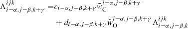 (D.19)
![Mathematical equation: $$ \begin{aligned} \Lambda _{{i,j-\beta ,k+\gamma }}^{{ijk}} =&c_{{i,j-\beta ,k+\gamma }}\tilde{w}_{\rm B}^{{i,j-\beta ,k+\gamma }} + d_{{i,j-\beta ,k+\gamma }}\nonumber \\& \times \Bigl [ \hat{w}_{\rm N}^{{i,j-\beta ,k+\gamma }} \Lambda _{{i-\alpha ,j-\beta ,k}}^{{ijk}} + \hat{w}_{\rm O}^{{i,j-\beta ,k+\gamma }} \Lambda _{{i,j-\beta ,k}}^{{ijk}}\nonumber \\&+ \hat{w}_{\rm Q}^{{i,j-\beta ,k+\gamma }} \Lambda _{{i-\alpha ,j-\beta ,k-\gamma }}^{{ijk}}\nonumber \\&+ \hat{w}_{\rm S}^{{i,j-\beta ,k+\gamma }} \Lambda _{{i-\alpha ,j-\beta ,k+\gamma }}^{{ijk}} \Bigr ] \end{aligned} $$](/articles/aa/full_html/2020/01/aa36584-19/aa36584-19-eq158.gif) (D.20)
(D.20)
![Mathematical equation: $$ \begin{aligned} \Lambda _{{i+\alpha ,j-\beta ,k+\gamma }}^{{ijk}} =&c_{{i+\alpha ,j-\beta ,k+\gamma }}\tilde{w}_{\rm A}^{{i+\alpha ,j-\beta ,k+\gamma }} + d_{{i+\alpha ,j-\beta ,k+\gamma }}\nonumber \\&\times \Bigl [ \hat{w}_{\rm M}^{{i+\alpha ,j-\beta ,k+\gamma }} \Lambda _{{i-\alpha ,j-\beta ,k}}^{{ijk}} + \hat{w}_{\rm N}^{{i+\alpha ,j-\beta ,k+\gamma }} \Lambda _{{i,j-\beta ,k}}^{{ijk}}\nonumber \\&+ \hat{w}_{\rm O}^{{i+\alpha ,j-\beta ,k+\gamma }} \Lambda _{{i+\alpha ,j-\beta ,k}}^{{ijk}} + \hat{w}_{\rm Q}^{{i+\alpha ,j-\beta ,k+\gamma }} \Lambda _{{i,j-\beta ,k-\gamma }}^{{ijk}}\nonumber \\&+ \hat{w}_{\rm S}^{{i+\alpha ,j-\beta ,k+\gamma }} \Lambda _{{i,j-\beta ,k+\gamma }}^{{ijk}} \Bigr ] \end{aligned} $$](/articles/aa/full_html/2020/01/aa36584-19/aa36584-19-eq159.gif) (D.21)
(D.21)
![Mathematical equation: $$ \begin{aligned} \Lambda _{{i-\alpha ,j,k+\gamma }}^{{ijk}} =&c_{{i-\alpha ,j,k+\gamma }}\tilde{w}_{\rm Q}^{{i-\alpha ,j,k+\gamma }} + d_{{i-\alpha ,j,k+\gamma }}\nonumber \\&\times \Bigl [ \hat{w}_{\rm C}^{{i-\alpha ,j,k+\gamma }} \Lambda _{{i-\alpha ,j-\beta ,k-\gamma }}^{{ijk}} + \hat{w}_{\rm F}^{{i-\alpha ,j,k+\gamma }} \Lambda _{{i-\alpha ,j-\beta ,k}}^{{ijk}}\nonumber \\&+ \hat{w}_{\rm I}^{{i-\alpha ,j,k+\gamma }} \Lambda _{{i-\alpha ,j-\beta ,k+\gamma }}^{{ijk}} +\hat{w}_{\rm O}^{{i-\alpha ,j,k+\gamma }} \Lambda _{{i-\alpha ,j,k}}^{{ijk}}\Bigr ] \end{aligned} $$](/articles/aa/full_html/2020/01/aa36584-19/aa36584-19-eq160.gif) (D.22)
(D.22)
![Mathematical equation: $$ \begin{aligned} \Lambda _{{i,j,k+\gamma }}^{{ijk}} =&a_{{i,j,k+\gamma }}w_{\rm O}^{{i,j,k+\gamma }} + d_{{i,j,k+\gamma }}\nonumber \\& \times \Bigl [ \hat{w}_{\rm B}^{{i,j,k+\gamma }} \Lambda _{{i-\alpha ,j-\beta ,k-\gamma }}^{{ijk}} + \hat{w}_{\rm C}^{{i,j,k+\gamma }} \Lambda _{{i,j-\beta ,k-\gamma }}^{{ijk}}\nonumber \\&+ \hat{w}_{\rm E}^{{i,j,k+\gamma }} \Lambda _{{i-\alpha ,j-\beta ,k}}^{{ijk}} + \hat{w}_{\rm F}^{{i,j,k+\gamma }} \Lambda _{{i,j-\beta ,k}}^{{ijk}}\nonumber \\&+ \hat{w}_{\rm H}^{{i,j,k+\gamma }} \Lambda _{{i-\alpha ,j-\beta ,k+\gamma }}^{{ijk}} + \hat{w}_{\rm I}^{{i,j,k+\gamma }} \Lambda _{{i,j-\beta ,k+\gamma }}^{{ijk}}\nonumber \\&+ \hat{w}_{\rm N}^{{i,j,k+\gamma }} \Lambda _{{i-\alpha ,j,k}}^{{ijk}} + \hat{w}_{\rm O}^{{i,j,k+\gamma }} \Lambda _{{ijk}}^{{ijk}}\nonumber \\&+ \hat{w}_{\rm Q}^{{i,j,k+\gamma }} \Lambda _{{i-\alpha ,j,k-\gamma }}^{{ijk}} + \hat{w}_{\rm S}^{{i,j,k+\gamma }} \Lambda _{{i-\alpha ,j,k+\gamma }}^{{ijk}} \Bigr ] \end{aligned} $$](/articles/aa/full_html/2020/01/aa36584-19/aa36584-19-eq161.gif) (D.23)
(D.23)
![Mathematical equation: $$ \begin{aligned} \Lambda _{{i+\alpha ,j,k+\gamma }}^{{ijk}} =&a_{{i+\alpha ,j,k+\gamma }}w_{\rm N}^{{i+\alpha ,j,k+\gamma }} + d_{{i+\alpha ,j,k+\gamma }}\nonumber \\& \times \Bigl [ \hat{w}_{\rm A}^{{i+\alpha ,j,k+\gamma }} \Lambda _{{i-\alpha ,j-\beta ,k-\gamma }}^{{ijk}} + \hat{w}_{\rm B}^{{i+\alpha ,j,k+\gamma }} \Lambda _{{i,j-\beta ,k-\gamma }}^{{ijk}}\nonumber \\&+\hat{w}_{\rm C}^{{i+\alpha ,j,k+\gamma }} \Lambda _{{i+\alpha ,j-\beta ,k-\gamma }}^{{ijk}} + \hat{w}_{\rm D}^{{i+\alpha ,j,k+\gamma }} \Lambda _{{i-\alpha ,j-\beta ,k}}^{{ijk}}\nonumber \\&+\hat{w}_{\rm E}^{{i+\alpha ,j,k+\gamma }} \Lambda _{{i,j-\beta ,k}}^{{ijk}} +\hat{w}_{\rm F}^{{i+\alpha ,j,k+\gamma }} \Lambda _{{i+\alpha ,j,k}}^{{ijk}}\nonumber \\&+\hat{w}_{\rm G}^{{i+\alpha ,j,k+\gamma }} \Lambda _{{i-\alpha ,j-\beta ,k+\gamma }}^{{ijk}} +\hat{w}_{\rm H}^{{i+\alpha ,j,k+\gamma }} \Lambda _{{i,j-\beta ,k+\gamma }}^{{ijk}}\nonumber \\&+\hat{w}_{\rm I}^{{i+\alpha ,j,k+\gamma }} \Lambda _{{i+\alpha ,j-\beta ,k+\gamma }}^{{ijk}} +\hat{w}_{\rm M}^{{i+\alpha ,j,k+\gamma }} \Lambda _{{i-\alpha ,j,k}}^{{ijk}}\nonumber \\&+ \hat{w}_{\rm N}^{{i+\alpha ,j,k+\gamma }} \Lambda _{{ijk}}^{{ijk}} + \hat{w}_{\rm O}^{{i+\alpha ,j,k+\gamma }} \Lambda _{{i+\alpha ,j,k}}^{{ijk}}\nonumber \\&+ \hat{w}_{\rm Q}^{{i+\alpha ,j,k+\gamma }} \Lambda _{{i,j,k-\gamma }}^{{ijk}} +\hat{w}_{\rm S}^{{i+\alpha ,j,k+\gamma }} \Lambda _{{i,j,k+\gamma }}^{{ijk}}\Bigr ] \end{aligned} $$](/articles/aa/full_html/2020/01/aa36584-19/aa36584-19-eq162.gif) (D.24)
(D.24)
![Mathematical equation: $$ \begin{aligned} \Lambda _{{i-\alpha ,j+\beta ,k+\gamma }}^{{ijk}} =&c_{{i-\alpha ,j+\beta ,k+\gamma }}\tilde{w}_{\rm P}^{{i-\alpha ,j+\beta ,k+\gamma }} + d_{{i-\alpha ,j+\beta ,k+\gamma }}\nonumber \\&\times \Bigl [ \hat{w}_{\rm C}^{{i-\alpha ,j+\beta ,k+\gamma }} \Lambda _{{i-\alpha ,j,k-\gamma }}^{{ijk}} + \hat{w}_{\rm F}^{{i-\alpha ,j+\beta ,k+\gamma }} \Lambda _{{i-\alpha ,j,k}}^{{ijk}}\nonumber \\&+ \hat{w}_{\rm I}^{{i-\alpha ,j+\beta ,k+\gamma }} \Lambda _{{i-\alpha ,j,k+\gamma }}^{{ijk}} + \hat{w}_{\rm L}^{{i-\alpha ,j+\beta ,k+\gamma }} \Lambda _{{i-\alpha ,j-\beta ,k}}^{{ijk}}\nonumber \\&+ \hat{w}_{\rm O}^{{i-\alpha ,j+\beta ,k+\gamma }} \Lambda _{{i-\alpha ,j+\beta ,k}}^{{ijk}} \Bigr ] \end{aligned} $$](/articles/aa/full_html/2020/01/aa36584-19/aa36584-19-eq163.gif) (D.25)
(D.25)
![Mathematical equation: $$ \begin{aligned} \Lambda _{{i,j+\beta ,k+\gamma }}^{{ijk}} =&a_{{i,j+\beta ,k+\gamma }}w_{\rm F}^{{i,j+\beta ,k+\gamma }} + d_{{i,j+\beta ,k+\gamma }}\nonumber \\&\times \Bigl [ \hat{w}_{\rm B}^{{i,j+\beta ,k+\gamma }} \Lambda _{{i-\alpha ,j,k-\gamma }}^{{ijk}} + \hat{w}_{\rm C}^{{i,j+\beta ,k+\gamma }} \Lambda _{{i,j,k-\gamma }}^{{ijk}}\nonumber \\&+\hat{w}_{\rm E}^{{i,j+\beta ,k+\gamma }} \Lambda _{{i-\alpha ,j,k}}^{{ijk}} + \hat{w}_{\rm F}^{{i,j+\beta ,k+\gamma }} \Lambda _{{ijk}}^{{ijk}}\nonumber \\&+ \hat{w}_{\rm H}^{{i,j+\beta ,k+\gamma }} \Lambda _{{i-\alpha ,j,k+\gamma }}^{{ijk}} + \hat{w}_{\rm I}^{{i,j+\beta ,k+\gamma }} \Lambda _{{i,j,k+\gamma }}^{{ijk}}\nonumber \\&+ \hat{w}_{\rm K}^{{i,j+\beta ,k+\gamma }} \Lambda _{{i-\alpha ,j-\beta ,k}}^{{ijk}} + \hat{w}_{\rm L}^{{i,j+\beta ,k+\gamma }} \Lambda _{{i,j-\beta ,k}}^{{ijk}}\nonumber \\&+ \hat{w}_{\rm N}^{{i,j+\beta ,k+\gamma }} \Lambda _{{i-\alpha ,j+\beta ,k}}^{{ijk}} + \hat{w}_{\rm O}^{{i,j+\beta ,k+\gamma }} \Lambda _{{i,j+\beta ,k}}^{{ijk}}\nonumber \\&+ \hat{w}_{\rm P}^{{i,j+\beta ,k+\gamma }} \Lambda _{{i-\alpha ,j-\beta ,k-\gamma }}^{{ijk}} + \hat{w}_{\rm Q}^{{i,j+\beta ,k+\gamma }} \Lambda _{{i-\alpha ,j+\beta ,k-\gamma }}^{{ijk}}\nonumber \\&+ \hat{w}_{\rm R}^{{i,j+\beta ,k+\gamma }} \Lambda _{{i-\alpha ,j-\beta ,k+\gamma }}^{{ijk}}\nonumber \\&+\hat{w}_{\rm S}^{{i,j+\beta ,k+\gamma }} \Lambda _{{i-\alpha ,j+\beta ,k-\gamma }}^{{ijk}} \Bigr ] \end{aligned} $$](/articles/aa/full_html/2020/01/aa36584-19/aa36584-19-eq164.gif) (D.26)
(D.26)
![Mathematical equation: $$ \begin{aligned} \Lambda _{{i+\alpha ,j+\beta ,k+\gamma }}^{{ijk}} =&a_{{i+\alpha ,j+\beta ,k+\gamma }}w_{\rm E}^{{i+\alpha ,j+\beta ,k+\gamma }} + d_{{i+\alpha ,j+\beta ,k+\gamma }} \nonumber \\&\times \Bigl [ \hat{w}_{\rm A}^{{i+\alpha ,j+\beta ,k+\gamma }} \Lambda _{{i-\alpha ,j,k-\gamma }}^{{ijk}} + \hat{w}_{\rm B}^{{i+\alpha ,j+\beta ,k+\gamma }} \Lambda _{{i,j,k-\gamma }}^{{ijk}}\nonumber \\&+\hat{w}_{\rm C}^{{i+\alpha ,j+\beta ,k+\gamma }} \Lambda _{{i+\alpha ,j,k-\gamma }}^{{ijk}} + \hat{w}_{\rm D}^{{i+\alpha ,j+\beta ,k+\gamma }} \Lambda _{{i-\alpha ,j,k}}^{{ijk}}\nonumber \\&+ \hat{w}_{\rm E}^{{i+\alpha ,j+\beta ,k+\gamma }} \Lambda _{{ijk}}^{{ijk}} + \hat{w}_{\rm F}^{{i+\alpha ,j+\beta ,k+\gamma }} \Lambda _{{i+\alpha ,j,k}}^{{ijk}}\nonumber \\&+ \hat{w}_{\rm G}^{{i+\alpha ,j+\beta ,k+\gamma }} \Lambda _{{i-\alpha ,j,k+\gamma }}^{{ijk}} + \hat{w}_{\rm H}^{{i+\alpha ,j+\beta ,k+\gamma }} \Lambda _{{i,j,k+\gamma }}^{{ijk}}\nonumber \\&+ \hat{w}_{\rm I}^{{i+\alpha ,j+\beta ,k+\gamma }} \Lambda _{{i+\alpha ,j,k+\gamma }}^{{ijk}} + \hat{w}_{\rm J}^{{i+\alpha ,j+\beta ,k+\gamma }} \Lambda _{{i-\alpha ,j-\beta ,k}}^{{ijk}} \nonumber \\&+ \hat{w}_{\rm K}^{{i+\alpha ,j+\beta ,k+\gamma }} \Lambda _{{i,j-\beta ,k}}^{{ijk}} + \hat{w}_{\rm L}^{{i+\alpha ,j+\beta ,k+\gamma }} \Lambda _{{i+\alpha ,j-\beta ,k}}^{{ijk}} \nonumber \\&+\hat{w}_{\rm M}^{{i+\alpha ,j+\beta ,k+\gamma }} \Lambda _{{i-\alpha ,j+\beta ,k}}^{{ijk}} + \hat{w}_{\rm N}^{{i+\alpha ,j+\beta ,k+\gamma }} \Lambda _{{i,j+\beta ,k}}^{{ijk}}\nonumber \\&+ \hat{w}_{\rm O}^{{i+\alpha ,j+\beta ,k+\gamma }} \Lambda _{{i+\alpha ,j+\beta ,k}}^{{ijk}} + \hat{w}_{\rm P}^{{i+\alpha ,j+\beta ,k+\gamma }} \Lambda _{{i,j-\beta ,k-\gamma }}^{{ijk}}\nonumber \\&+ \hat{w}_{\rm Q}^{{i+\alpha ,j+\beta ,k+\gamma }} \Lambda _{{i,j+\beta ,k-\gamma }}^{{ijk}} + \hat{w}_{\rm R}^{{i+\alpha ,j+\beta ,k+\gamma }} \Lambda _{{i,j-\beta ,k+\gamma }}^{{ijk}}\nonumber \\&+\hat{w}_{\rm S}^{{i+\alpha ,j+\beta ,k+\gamma }} \Lambda _{{i,j+\beta ,k+\gamma }}^{{ijk}} \Bigr ]. \end{aligned} $$](/articles/aa/full_html/2020/01/aa36584-19/aa36584-19-eq165.gif) (D.27)
(D.27)
Since the integration and interpolation coefficients need to be calculated only once at each considered grid point (here denoted by (u, v, w), to avoid confusion), we obtain the Λ-matrix coefficients by substituting indices. For Eq. (D.1), we find:
 (D.28)
and proceed analogously for all other elements in Eqs. (D.2)–(D.27). Thus, the ALO can be calculated in parallel to the formal solution scheme.
All Tables
Mean relative error (defined in Sect. 4.2) of the mean intensity for a zero-opacity model, obtained using the Lebedev, Gauss-Legendre, and trapezoidal integration method, the latter with nodes from Lobel & Blomme (2008).
Mean and maximum relative errors of the FVM and SClin, SCbez methods, when applied to spherically symmetric test models.
All Figures
|
Fig. 1. Geometry of the SC method for a particular ray with direction n propagating from the upwind point u(ijk) to a considered grid point p(ijk). The downwind point d(ijk) is required to set the slope of a Bézier curve representing the opacities and source functions along the ray. The middle and lower panel display all possible downwind and upwind intersection surfaces for a short characteristic at a grid point p(ijk). For rays intersecting the xy-, xz-, and yz-planes, the 2D Bézier interpolation is obtained from given quantities at grid points located in the cyan, red, and magenta shaded surfaces, respectively. The coordinate system is indicated at the upper left, where α, β, γ determine the direction of the coordinate-axes and are defined in Sect. 3.3. |
| In the text | |
|
Fig. 2. Boundary conditions for rays propagating in the xz-plane at y-level (j) with three different directions n1, n2, n3, and upwind points u1, u2, u3. For point u1, the intensity is set to |
| In the text | |
|
Fig. 3. Searchlight-beam test for direction n = (1, 0, 1) and a typical grid with Nx = Ny = Nz = 133 grid points. Upper panel: contour plot of the specific intensity as calculated with the SC method using Bézier interpolations in the xz-plane (cf. Paper I, Fig. 3, for the finite-volume method). Middle panel: specific intensity through the perpendicular area indicated by the straight line in the upper panel. The blue, red, and green profiles correspond to the FVM, SClin, and SCbez methods, respectively. The dashed line indicates the theoretical profile. Bottom panel: as middle panel, but along the centre of the searchlight beam. We note that the SC methods reproduce the exact solution at the centre of the beam, whereas the FVM solution decreases significantly for r ≳ 2.5 R*. |
| In the text | |
|
Fig. 4. Photon flux as a function of direction angle ϕ (with fixed θ = 45°) through corresponding perpendicular areas, and with the opacity set to zero. The central distance of all areas to the stellar surface has been set to 2 R*. The same colour coding as in Fig. 3 has been used. |
| In the text | |
|
Fig. 5. Convergence behaviour of the standard spherically symmetric model calculated with the 3D FVM (blue) and the 3D SC method using linear (red) or Bézier (green) interpolations. Left and right panels: convergence behaviour of the continuum and line transfer for ϵC = ϵL = 10−6, respectively. While the upper row displays the optically thin models with kC = 10 and kL = 10, the lower row has been calculated using kC = 100 and kL = 105. Different acceleration techniques have been applied, where the NN-ALO is implemented only for the SC method. |
| In the text | |
|
Fig. 6. Solutions for the standard spherically symmetric models as calculated with the 3D FVM (blue) and 3D SC methods using linear (red) or Bézier (green) interpolations, compared to an accurate 1D solution (black solid line). The dots represent the solutions at specific grid points (with different latitudes and longitudes), where only a subset of all grid points is displayed to compress the image. Corresponding errors are indicated at the bottom of each chart. Top panel: mean intensity for the continuum transfer as a function of radius, with ϵC = 10−6, and kC = [1, 10, 100] from left to right. Bottom panel: line source function with ϵL = 10−6, and kL = [100, 103, 105] from left to right. |
| In the text | |
|
Fig. 7. Emergent flux profiles of an intermediate (kL = 103, top panel) and strong (kL = 105, bottom panel) line. The blue, red, and green curves correspond to the solution of the FVM, SClin, and SCbez methods, respectively. The reference profile (black solid line) has been derived from the “exact” 1D source function interpolated onto the 3D Cartesian grid. Corresponding relative and absolute errors are shown at the bottom of each chart. For all profiles, the continuum level has been determined from a zero-opacity model. |
| In the text | |
|
Fig. 8. Contours of the density in the xz-plane (z being the rotation axis) for a prototypical rotating O star with L* = 106 L⊙, M* = 52.5 M⊙, Rp = 19 R⊙, and vrot = 432 km s−1 (corresponding to Ω = 0.9). The density has been scaled by values from the non-rotating model with Ω = 0. While the thick solid line corresponds to the surface of the (distorted) star, the dashed line would correspond to a spherical surface. Additionally, the velocity vectors are displayed. |
| In the text | |
|
Fig. 9. Density and radial velocity as a function of distance from the stellar surface in polar (first and third panel) and equatorial (second and fourth panel) regions, for different rotation parameters Ω. |
| In the text | |
|
Fig. 10. Predicted emergent flux profiles for the rotating star models with Ω = [0, 0.5, 0.7, 0.9] (see Table 3). Upper and lower panels: intermediate and strong line with kL = 103 and kL = 105, respectively. The inclination angle has been set to sin(i) = [0, 0.707, 1] from left to right. |
| In the text | |
|
Fig. 11. Continuum fluxes for different inclinations sin(i) = [0, 0.707, 1] from left to right, and different rotation parameters (using the same colour coding as in Fig. 10). The continuum fluxes have been scaled by the corresponding flux obtained from the non-rotating model. |
| In the text | |
|
Fig. 12. Predicted emergent flux profiles for the rotating star models with Ω = [0.5, 0.6, 0.7, 0.8, 0.9], and different inclination angles such that v sin (i) = 200 km s−1 for all models. The upper and lower panels display the intermediate (kL = 103) and strong (kL = 105) line, respectively. |
| In the text | |
|
Fig. A.1. Probability density functions of radial (dashed) and x (solid) coordinates for different spherical and Cartesian grids. In this example, two spherical grids are given in 2D as input to our 3D code, with uniformly (black) or logarithmically (red) distributed r-coordinates, and a uniformly distributed polar angle. The corresponding distributions of x-coordinates are calculated within our grid construction procedure (see text). Large values of the probability density functions correspond to a high resolution of x and r-coordinates. |
| In the text | |
|
Fig. B.1. Bézier curves (solid lines) for three given points b0, b1, b2. The blue, red, and green lines represent the resulting curves for different control points b1. The straight connections of the control points with the data points are indicated by the dotted lines. |
| In the text | |
|
Fig. B.2. Different interpolation techniques for a set of three data points at x-coordinates indicated by the dotted vertical lines. The solid and dashed lines correspond to the interpolation in the different intervals [xi − 1, xi] and [xi, xi + 1], respectively. Linear interpolations, quadratic interpolations (connecting all three data points), and a monotonic Bézier curve (with ω calculated from Eq. (B.5) in the interval [xi − 1, xi]) are indicated in red, blue, and green. Since the quadratic interpolation is already monotonic in the interval [xi, xi + 1], the monotonic Bézier curve coincides with the dashed, blue line. Control points are indicated with coloured asterisks. |
| In the text | |
|
Fig. C.1. 2D interpolation for upwind or downwind quantities required in the cyan shaded area. The 2D Bézier interpolation consists of three 1D interpolations to obtain the values at the desired x-coordinate (indicated by red dots), followed by a 1D interpolation along the y-coordinate using the obtained values at the red dots. |
| In the text | |
|
Fig. D.1. 2D example for calculating the ΛΩ, ν-matrix elements at a grid point (i − α, j − β) (upper panel) and (i, j − β) (lower panel). The matrix elements correspond to the intensity at the considered grid points calculated for a source function Sij = 1 and zero everywhere else. For such a configuration, the downwind source function is interpolated from grid points indicated with the green dots, while the upwind source function and upwind intensity are obtained from the red dots (for simplicity we here assume linear interpolations for determining upwind and downwind quantities). We emphasize that the upwind intensity vanishes only when considering the grid point (i − α, j − β). |
| In the text | |
Current usage metrics show cumulative count of Article Views (full-text article views including HTML views, PDF and ePub downloads, according to the available data) and Abstracts Views on Vision4Press platform.
Data correspond to usage on the plateform after 2015. The current usage metrics is available 48-96 hours after online publication and is updated daily on week days.
Initial download of the metrics may take a while.