| Issue |
A&A
Volume 627, July 2019
|
|
|---|---|---|
| Article Number | A17 | |
| Number of page(s) | 15 | |
| Section | Planets and planetary systems | |
| DOI | https://doi.org/10.1051/0004-6361/201935220 | |
| Published online | 25 June 2019 | |
Inverse Lidov-Kozai resonance for an outer test particle due to an eccentric perturber
1
Instituto de Astrofísica de La Plata,
CCT La Plata-CONICET-UNLP Paseo del Bosque s/n (1900),
La Plata, Argentina
e-mail: This email address is being protected from spambots. You need JavaScript enabled to view it.
2
Facultad de Ciencias Astronómicas y Geofísicas, Universidad Nacional de La Plata Paseo del Bosque s/n (1900),
La Plata, Argentina
3
Department of Physics and Astronomy, University of California,
Los Angeles,
CA
90095,
USA
Received:
6
February
2019
Accepted:
19
April
2019
Abstract
Aims. We analyze the behavior of the argument of pericenter ω2 of an outer particle in the elliptical restricted three-body problem, focusing on the ω2 resonance or inverse Lidov-Kozai resonance.
Methods. First, we calculated the contribution of the terms of quadrupole, octupole, and hexadecapolar order of the secular approximation of the potential to the outer particle’s ω2 precession rate (dω2∕dτ). Then, we derived analytical criteria that determine the vanishing of the ω2 quadrupole precession rate (dω2/dτ)quad for different values of the inner perturber’s eccentricity e1. Finally, we used such analytical considerations and described the behavior of ω2 of outer particles extracted from N-body simulations developed in a previous work.
Results. Our analytical study indicates that the values of the inclination i2 and the ascending node longitude Ω2 associated with the outer particle that vanish (dω2/dτ)quad strongly depend on the eccentricity e1 of the inner perturber. In fact, if e1 < 0.25 (>0.40825), (dω2/dτ)quad is only vanished for particles whose Ω2 circulates (librates). For e1 between 0.25 and 0.40825, (dω2/dτ)quad can be vanished for any particle for a suitable selection of pairs (Ω2, i2). Our analysis of the N-body simulations shows that the inverse Lidov-Kozai resonance is possible for small, moderate, and high values of e1. Moreover, such a resonance produces distinctive features in the evolution of a particle in the (Ω2, i2) plane. In fact, if ω2 librates and Ω2 circulates, the extremes of i2 at Ω2 = 90° and 270° do not reach the same value, while if ω2 and Ω2 librate, the evolutionary trajectory of the particle in the (Ω2, i2) plane shows evidence of an asymmetry with respect to i2 = 90°. The evolution of ω2 associated with the outer particles of the N-body simulations can be very well explained by the analytical criteria derived in our investigation.
Key words: planets and satellites: dynamical evolution and stability / minor planets, asteroids: general / methods: numerical
© ESO 2019
1 Introduction
The approximation of secular dynamics is a powerful tool for studying a wide diversity of astrophysical problems. In particular, the works carried out by Lidov (1962) and Kozai (1962) were the first ones aimed at exploring the secular perturbations produced by a far away massive planet on a circular orbit over an inner test particle. In their works, the authors showed that, if the minimum inclination of the inner massless particle is between 39.23° and 140.77°, its eccentricity e, inclination i, and argument of pericenterω experience coupled oscillations. This secular effect associated with the evolution of the inner test particle is known as the Lidov-Kozaimechanism.
When the hypothesis of the circular orbit for the outer perturber relaxes, interesting dynamical modes of behavior of the inner test particle become visible. Several authors have focused on the so-called inner eccentric Lidov-Kozai mechanism, analyzing the evolution of an inner particle in the elliptical restricted three-body problem. In particular, Harrington (1968), Soderhjelm (1984), Krymolowski & Mazeh (1999), Ford et al. (2000), and Naoz et al. (2013) derived general expressions for the secular hamiltonian, while Lithwick & Naoz (2011) and Katz et al. (2011) explored the case of the dynamical evolution of an inner test particle that orbits a star under the effects of an outer and eccentric massive perturber up to the octupole level of secular approximation. In such studies, it is possible understand that if the outer massive perturber has an eccentric orbit, the vertical angular momentum of the inner massless particle is not conserved and thus, its orbital plane can change the orientation from prograde to retrograde and back again, reaching very high eccentricities close to the unity.
The study of the secular dynamics of an outer test particle in the elliptical restricted three-body problem also shows significant results concerning the evolution of its orbital parameters. In this sense, Ziglin (1975) was the first to describe several aspects concerning the so-called outer eccentric Lidov-Kozai mechanism, analyzing the secular evolution of a distant planet orbiting a binary star system. From a doubly averaged disturbing function and under the context of the restricted three-body problem, the author showed that the evolution of the inclination i and the ascending node longitude Ω of the outerplanet is coupled, and furthermore, the width of libration region associated with Ω only depends on the eccentricity of the inner binary. Recently, Farago & Laskar (2010) analyzed the dynamical evolution for a distant test particle that orbits a central star under the gravitational effects of an internal massive planet up to the quadrupole level of the secular approximation. These authors confirmed the results obtained by Ziglin (1975) and extended their studies to the general case of the three-body problem.
The outer restricted three-body problem was also studied by Li et al. (2014), who obtained general solutions to some orbital parameters up to the quadrupole level of the secular approximation. Furthermore, Li et al. (2014) explored the contribution of the octupole term of the secular hamiltonian and determined the evolution of the eccentricity of the outer massless particle for slightly inclined orbits and near polar configurations, and different values associated with the inner binary’s eccentricity.
More recently, Naoz et al. (2017) and Zanardi et al. (2017) carried out two joint works aimed at studying the effects produced by an inner and eccentric massive perturber over the dynamical evolution of an outer massless particle, which both orbit around a given central star. On the one hand, Naoz et al. (2017) derived analytical expressions up to the octupole level of the secular approximation for an outer test particle in the elliptical restricted three-body problem. From this, the authors showed that the analysis of the system under consideration is consistent with that derived by Ziglin (1975) up to the quadrupole level of the approximation, and they discussed in detail the sensitivity of the octupole terms of the secular hamiltonian to the results. On the other hand, Zanardi et al. (2017) studied the formation and evolution of outer small body populations in systems that suffer strong scattering events between giant planets around 0.5 M⊙ stars from N-body simulations. In particular, the authors focused the investigation on systems composed of a single inner Jupiter-mass planet and a far away reservoir of small bodies after the dynamical instability event. According to such a study, a natural result observed in these systems is the generation of particles with prograde and retrograde orbits whose ascending node longitude Ω circulates, and particles whose orbit plane flips1 from prograde to retrograde and back again throughout the evolution with coupled librations associated with Ω. It is worth noting that the comparative analysis carried out by Zanardi et al. (2017) shows that the numerical results obtained in their research are supported by the analytical expressions derived by Naoz et al. (2017).
Then, Zanardi et al. (2018) analyzed the role of general relativity (GR) on outer small body reservoirs under the effects of an inner and eccentric Jupiter-mass planet around low-mass stars. From N-body simulations and analytical criteria, the authors showed that the GR may significantly modify the dynamical properties of the outer test particles. In fact, if the GR is included in the analysis, the range of prograde (retrograde) inclinations of the libration region associated with the ascending node longitude is reduced (increased) in comparison with that observed in the absence of GR.
Finally, Vinson & Chiang (2018) performed a study concerning the secular dynamics of an outer test particle in the elliptical restricted three-body problem from the expansion of the potential up to hexadecapolar level of the approximation. In this research, the authors described the quadrupole orbital-flipping resonance, the octupole resonances associated with librations of ω + Ω and ω − Ω around 0°, and the hexadecapolar ω resonance, in which ω librates around 90° or 270° and is the so-called inverse Lidov-Kozai resonance.
The inverse Lidov-Kozai resonance in the transneptunian region of the solar system was analyzed by Gallardo et al. (2012) assuming the gravitational effects of the giant planets on circular and coplanar orbits. As we mentioned in the previous paragraph, Vinson & Chiang (2018) extended the study of the inverse Lidov-Kozai resonance for the case of an inner perturber moving on an eccentric orbit. These authors found the inverse Lidov-Kozai resonance only up to a value of the inner perturber’s eccentricity of 0.1 in N-body experiments. However, Zanardi et al. (2017) noted the existence of a few flipping particles that experience simultaneous librations of the ascending node longitude Ω and the argument of pericenterω, which are associated with an inner perturber’s eccentricity greater than 0.2 in their N-body simulations.
From such results, the main goal of this research is to analyze in detail the inverse Lidov-Kozai resonance as a function of the inner perturber’s eccentricity from analytical criteria and N-body simulations. Working on the basis of the elliptical restricted three-body problem, we will show that the inverse Lidov-Kozai resonance can be found for small, moderate, and high values of the orbital eccentricity associated with the inner perturber.
The present paper is structured as follows. In Sect. 2, we present a brief, up-to-date overview of the outer eccentric Lidov-Kozai mechanism. The analytical treatment concerning the precession rate of the argument of pericenter of an outer test particle is described in Sect. 3. A detailed analysis of results derived from N-body simulations is shown in Sect. 4. Finally, Sect. 5 describes the discussions and conclusions of our study.
2 Overview
Recently, Naoz et al. (2017) analyzed in detail the secular dynamics of an outer test particle evolving under the gravitational influence of an inner and eccentric perturber of mass m1 orbiting a central star of mass m0. If the orbital parameters e2, i2, ω2, and Ω2 represent the eccentricity, the inclination with respect to the inner orbit, the argument of pericenter, and the ascending node longitude of the outer test particle relative to the inner perturber’s periapse, respectively, the equations of motion can be written as partial derivatives of an energy function f in the following way:
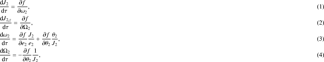
where θ2 = cos i2,  ,
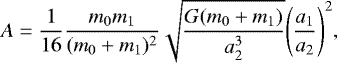
,  , and τ is a parameter proportionalto the true time t, which is given by τ = At, with
 (5)
(5)
G being the gravitational constant, and a1 and a2 the semimajor axis of the inner perturber and the outer test particle, respectively. The energy function f derived by Naoz et al. (2017) up to the octupole level of the secular approximation is given by
 (6)
(6)
where the ɛ parameter is written by
 (7)
(7)
and the functions fquad and foct 2 adopt the expressions
 (8)
(8)
![Mathematical equation: \begin{eqnarray*} f_{\text{oct}} &=& \frac{-15e_1}{4(1-e^2_2)^{3/2}}\Bigg\{10(1-e^2_1)\theta_2(1-\theta^2_2)\sin\omega_2\sin\Omega_2 \Bigg.\nonumber\\ &&+\, \frac{1}{2}\bigg[2+19e^2_1-5(2+5e^2_1)\theta^2_2-35e^2_1(1-\theta^2_2)\cos(2\Omega_2)\bigg]\nonumber\\ &&\times\, \Bigg.(\theta_2\sin\omega_2\sin\Omega_2-\cos\omega_2\cos\Omega_2)\Bigg\}, \end{eqnarray*}](/articles/aa/full_html/2019/07/aa35220-19/aa35220-19-eq12.png) (9)
(9)
where e1 is the eccentricity of the inner massive perturber.
At the quadrupole level of the secular approximation, Naoz et al. (2017) found that the inclination i2 and the ascending node longitude Ω2 of the outer test particle evolve with precession rates given by di2∕dτ ∝ sin(2Ω2) and dΩ2∕dτ ∝ θ2. According to this, on the one hand, the inclination i2 adopts extreme values for Ω2 = 0°, 90° or 270°. On the other hand, the ascending node longitude Ω2 reaches minimum and maximum values for i2 = 90°, which represents a very important result to understand the secular behavior of an outer test particle. In fact, from this, the ascending node longitude Ω2 can evolve following two different regimes: circulation or libration. In a circulation trajectory, Ω2 adopts values between 0° and 360°, and the outer test particle always evolves on prograde or retrograde orbits. In a libration trajectory, Ω2 is constrained between two specific values, and the orbital plane of the outer test particle flips from prograde to retrograde and back again along its evolution. This orbit-flipping quadrupole resonance, in which Ω2 librates around 90° or 270°, was mentioned originally in the pioneering work carried out by Ziglin (1975) and a detailed description of this can be found in Naoz et al. (2017).
The critical trajectory that divides the circulation and libration regimes in an inclination i2 versus ascending node longitude Ω2 plane is called the separatrix. According to that described in last paragraph, the separatrix has associated a value of i2 = 90° for Ω2 = 0°. By taking into account that the extreme values of the inclination i2 on the separatrix (hereafter referred by  ) are obtained for Ω2 = 90° or 270°, the conservation of energy at the quadrupole level of the approximation indicates that fquad(Ω2 = 0°, i2 = 90°) = fquad(Ω2 = 90° or 270
 , where fquad is given by Eq. (8). From this,
 (10)
(10)
and then, the range of inclinations that lead to libration trajectories of Ω2 has a width Δi2 given by
 (11)
(11)
According to this expression, the more eccentric the inner perturber, the larger the range of inclinations that lead to libration trajectories of Ω2. In particular, it is worth remarking that a perturber on a circular orbit cannot produce this orbit-flipping resonance that involves librations of Ω2 since the width Δi2 = 0°.
Recently, Vinson & Chiang (2018) studied the dynamics of an outer test particle in the secular three-body problem expanding the hamiltonian of the system up to hexadecapolar order. To do this, the authors adapted the disturbing function for an outer perturber derived by Yokoyama et al. (2003). According to this, the hexadecapolar term of the secular approximation associated with the energy function f for an outer test particle adopts the expression3
 (12)
(12)
where c3 is given by
 (13)
(13)
and
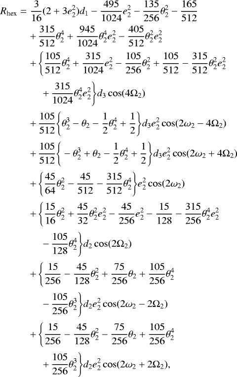 (14)
(14)
where

From the analysis carried out by Vinson & Chiang (2018), it is worth noting that the ω2 resonance or inverse Lidov-Kozai resonance appears at hexadecapole order in the secular treatment due to the existence of the term in Eq. (14) proportionalto  .
.
Vinson & Chiang (2018) derived interesting conclusions concerning the inverse Lidov-Kozai resonance for different values corresponding to the eccentricity e1 of the inner perturber. In fact, from a secular analysis truncated up to the hexadecapolar order, the authors inferred that the inverse Lidov-Kozai resonance persists up to a value of e1 = 0.3. However, from N-body simulations, the authors found the inverse Lidov-Kozai resonance only up to a value of e1 = 0.1. From these results, Vinson & Chiang (2018) suggested that the inverse Lidov-Kozai resonance seems to disappear at higher e1 being overwhelmed by the octupole effects. It is important to remark that the experiments carried out by these authors did not use a wide range of initial conditions associated with the orbital parameters of the outer test particle for each value of the eccentricity of the inner perturber.
3 Determination of the ω2 precession rate
In the previous section, we described the expression of the energy function f associated with an outer test particle orbiting around a central star and evolving under the influence of an inner perturber with an arbitrary eccentricity. In particular, we presented the quadrupole and octupole terms of the energy function calculated by Naoz et al. (2017), and the hexadecapolar term derived by Vinson & Chiang (2018). From such expressions and the equations of motion given by Eqs. (1)–(4), it is possible to determine the change rate of the eccentricity e2, the inclination i2, the argument of pericenter ω2, and the ascending node longitude Ω2 associated with the outer test particle. As we have said before, our main research focuses on the inverse Lidov-Kozai resonance, for which we are only interested in computing the ω2 precession rate in the present study.
3.1 General treatment
Taking into account the quadrupole, octupole, and hexadecapolar terms of the energy function, it is possible to determine the contribution of each order of the secular approximation to the ω2 precession rate. Thus, the ω2 quadrupole precession rate is given by
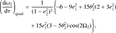 (18)
(18)
Then, the contribution of the octupole term to the ω2 precession rate adopts the expression
![Mathematical equation: \begin{eqnarray*} \Bigg(\frac{\textrm{d}\omega_2}{\textrm{d}\tau}\Bigg)_{\text{oct}}\Bigg.&=& \frac{\epsilon}{(1-e^2_2)^{1/2}}\Bigg\{(4+\frac{1}{e^2_2})f_{\text{oct}}\Bigg\} \nonumber \\ &&-\, \frac{15\epsilon e_1 \theta_2}{4(1-e^2_2)^2}\Bigg\{10(1-e^2_1)(1-3\theta^2_2)\sin\omega_2\sin\Omega_2 \nonumber \\ &&+\, \frac{1}{2}\bigg[-10\theta_2(2+5e^2_1)+70e^2_1\theta_2\cos(2\Omega_2)\bigg] \nonumber \\ &&\times\, (\theta_2\sin\omega_2\sin\Omega_2-\cos\omega_2\cos\Omega_2) \nonumber \\ &&+\, \frac{1}{2}\bigg[2+19e^2_1-5\theta^2_2(2+5e^2_1) \bigg.\nonumber \\ &&-\, \bigg.\Bigg.35e^2_1(1-\theta^2_2)\cos(2\Omega_2)\bigg]\sin\omega_2\sin\Omega_2\Bigg\}.\end{eqnarray*}](/articles/aa/full_html/2019/07/aa35220-19/aa35220-19-eq23.png) (19)
(19)
Finally,the contribution of the hexadecapolar term to the ω2 precession rate is given by
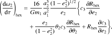 (20)
(20)
where c3 and Rhex are given by Eqs. (13) and (14), respectively, and
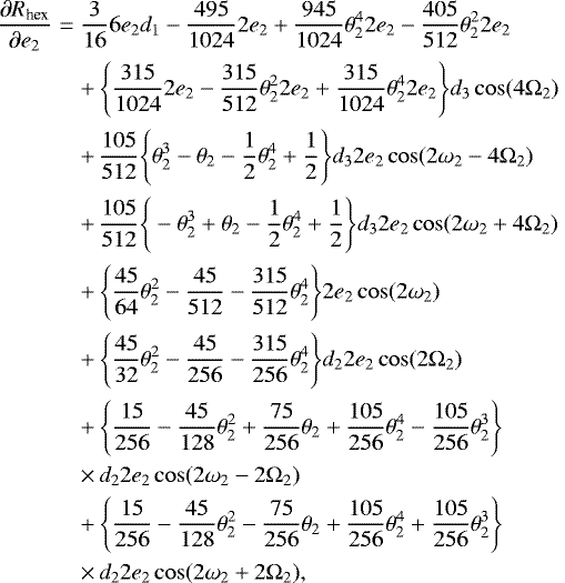 (21)
(21)
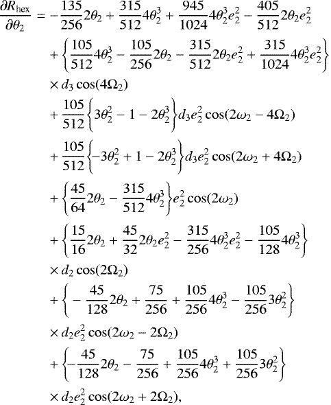 (22)
(22)
 (23)
(23)
Once  ,
,  , and
, and  are calculated from Eqs. (18), (19), and (20), respectively, the ω2 precession rate up to the hexadecapolar order of the secular approximation is derived by
 (24)
(24)
It is important to remark that if we want to compute the ω2 precession rate with respect to the true time t, it is necessary to multiply Eq. (24) by the factor A given by Eq. (5).
3.2 Vanishing of the ω2 quadrupole precession rate
In general terms, in a secular treatment, the quadrupole precession rate of the argument of pericenter of the outer test particle is that of greater magnitude since it is proportional to  . Thus, it is very interesting to determine the orbital parameter space that leads to the vanishing of
  .
.
Setting  in Eq. (18), we find that the values of the inclination i2 that satisfy this condition are given by
![Mathematical equation: \begin{eqnarray*} i_2=\arccos\left\{\pm\sqrt{\frac{2+3e^2_1[1-5\cos(2\Omega_2)]}{10+5e^2_1[3-5\cos(2\Omega_2)]}}\right\}.\end{eqnarray*}](/articles/aa/full_html/2019/07/aa35220-19/aa35220-19-eq35.png) (25)
(25)
This expression allows us to derive several considerations of interest concerning the temporal evolution of ω2. The simplest case is produced when the orbit of the inner perturber is circular. In fact, if e1 = 0, the quadrupole precession rate of the argument of pericenter of the outer test particle vanishes for orbital inclinations i2 = 63.4° and 116.6°. This result is consistent with the critical inclinations that lead to the inverse Lidov-Kozai resonance derived by Gallardo et al. (2012), who analyzed the Kozai dynamics in the transneptunian region of the solar system taking into account the gravitational perturbations of the giant planets moving in circular and coplanar orbits. More recently, Vinson & Chiang (2018) studied the outer elliptical restricted three-body problem and also determined such critical inclinations associated with the vanishing of the ω2 quadrupole precession rate analyzing the particular case of an inner perturber on a circular orbit.
The problem is more complex when the inner perturber’s orbit is eccentric. In fact, if e1 > 0, the values of the inclination i2 that vanish the quadrupole precession rate of the argument of pericenter of the outer test particle depend on the ascending node longitude Ω2. The blue curve illustrated in Fig. 1 represents the pairs (Ω2, i2) that vanish the ω2 quadrupole precession rate for different values of the eccentricity e1 associated with the inner perturber. Moreover, the red curve illustrates the separatrix, while the red shaded region represents the pairs (Ω2, i2) that lead to the orbit-flipping resonance.
From this, Fig. 1 allows us to appreciate important results concerning the vanishing of the ω2 quadrupole precession rate. On the one hand, for a value of e1 < e1,NF, all pairs (Ω2, i2) that vanish the quadrupole precession rate of the argument of pericenter ω2 are located outside the red shaded region that corresponds to orbital flips. To calculate e1,NF, we equate Eq. (25) at Ω2 = 90° and Eq. (10), which implies that  . According to this expression, e1,NF adopts a value of 0.25.
On the other hand, it is also important to remark that for a value of e1 > e1,F, the ω2 quadrupole precession rate is vanished only for pairs (Ω2, i2) associated with the orbital flip, red-shaded region. As Fig. 1 shows, to determine e1,F, it is enough to evaluate Eq. (25) at (Ω2 = 0°, i2 = 90°), which is a pair corresponding to the separatrix. This condition implies that  , which is satisfied for a value of e1,F = 0.40825.
This simple analysis allows us to observe that the eccentricity e1 of the inner perturber determines what kind of outer test particles vanish the ω2 quadrupole precession rate. In fact, if the perturber’s eccentricity e1 < e1,NF = 0.25, the ω2 quadrupole precession rate is only vanished for outer test particles on prograde and retrograde orbits whose Ω2 evolves on a circulatory regime, while when e1 > e1,F = 0.40825, only outer test particles on flipping orbits vanish the ω2 quadrupole precession rate. For perturbers with eccentricities e1 between 0.25 and 0.40825, the ω2 quadrupole precession rate can be vanished for outer test particles on prograde and retrograde orbits whose Ω2 circulates, as well as for particles that experience an orbit-flipping resonance, for values of the pair (Ω2, i2) that satisfy Eq. (25).
In the next section, we make use of these analytical considerations with the aim of describing results obtained from N-body simulations. In fact, we use the expressions of the ω2 precession rate obtained in Sect. 3.1 and the criterion derived from the vanishing of the ω2 quadrupole precession rate to analyze the dynamical behavior of outer test particles that orbit around a central star and evolve under the effects of an inner and eccentric massive perturber in a given set of N-body experiments.
4 Results of N-body simulations
Recently, Zanardi et al. (2017) carried out N-body simulations4 aimed at studying the behavior of planetary systems that initially harbor three Jupiter-mass giants located close to their dynamical instability limit and an outer disk of test particles on quasicircular and coplanar orbits around a 0.5 M⊙ star. In thiswork, the authors analyzed the dynamical properties of such systems after undergoing strong planetary scattering events involving the three gaseous giants, and they focused their study on a set of N-body simulations, in which a single Jupiter-mass planet survives after the dynamical instability event. In particular, Zanardi et al. (2017) studied in detail a total of 12 N-body simulations, each of which began with 1000 test particles, being some of them removed during the evolution due to strong scattering events from collisions with the planets or the central star, or ejections from the system. In general terms, the 12 N-body simulations developed by Zanardi et al. (2017) produce systems with outer reservoirs composed of three different kinds of test particles: (1) particles on prograde orbits and whose Ω2 circulates (hereafter Type-P particles), (2) particles on retrograde orbits and whose Ω2 circulates (hereafter Type-R particles), and (3) particles whose orbital plane flips from prograde to retrograde and back again along their evolution and whose Ω2 librates (hereafter Type-F particles).
In the present work, we study the evolution of the argument of pericenter ω2 of the surviving outer test particles associated with the 12 N-body simulations analyzed in detail by Zanardi et al. (2017), in each of which a single Jupiter-mass planet survives in the system with different values of the semimajor axis a1 and the eccentricity e1. In particular, our main research is based on outer test particles with values of (a1 ∕a2) and ɛ parameter ≲ 0.1. With these conditions, we seek to minimize the existence of non-secular effects in the sample of test particles of work extracted from the N-body simulations.
It is important to remark that the Jupiter-mass planets surviving in the 12 N-body simulations that represent our sample of work show a wide diversity of orbital eccentricities. From such a sample, we can distinguish three different sets of N-body simulations:
-
Set 1: two of 12 N-body simulations, in which the inner Jupiter-mass planet has an eccentricity e1 < e1,NF = 0.25,
-
Set 2: one of 12 N-body simulations, in which the inner Jupiter-mass planet has an eccentricity 0.25 < e1 < 0.40825, and
-
Set 3: nine of 12 N-body simulations, in which the inner Jupiter-mass planet has an eccentricity e1 > e1,F = 0.40825.
Taking into account the analytical considerations derived in Sect. 3, we analyze the evolution of the argument of pericenter ω2 of the Type-P, -R, and -F outer test particles in each of these three different sets of N-body simulations. It is worth mentioning that we do not find test particles of interest concerning the evolution of the argument of pericenter ω2 in the N-body simulation associated with Set 2. From this, our study focuses on the Sets 1 and 3 of N-body simulations, which show test particles with a wide diversity of dynamical behavior.
We want to note two very important points concerning the N-body simulations used in the present research. On the one hand, the initial conditions of the test particles refer to orbital parameters immediately after the dynamical instability event, when a single Jupiter-mass planet survives in the system. In fact, we study the dynamical properties of each test particle in the framework of a restricted three-body problem (star + planet + test particle) and its initial conditions must correspond to such a system. A detailed discussion on this is developed by Zanardi et al. (2017), and an illustration of the initial conditions of the test particles associated with the 12 N-body simulations used in the present work can be found in Fig. 2 of Zanardi et al. (2018). On the other hand, in order to compare properly the numerical results to the analytical expressions obtained in Sect. 3, we emphasize that the orbital parameters of the outer test particles and the surviving planet of each N-body simulation are assumed to be referenced to the barycenter and invariant plane of the system (star + planet), whose x-axis is selected to coincide with the surviving planet’s periapse. To do this, we set the longitude of pericenter of the inner perturber ϖ1 = 0 in agreement with Naoz et al. (2017) and Vinson & Chiang (2018).
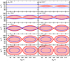 |
Fig. 1 Pairs (Ω2, i2) that vanish the ω2 quadrupole precession rate are illustrated by a blue curve for different values of the eccentricity e1 associated with the inner perturber, which is specified at the top left corner of every panel. For each scenario, the separatrix of the system, which is computed up to the quadruple level of the secular approximation, is represented by a red curve, while the red shaded region illustrates the pairs (Ω2, i2) that lead to the orbit-flipping quadrupole resonance. |
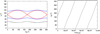 |
Fig. 2 Left panel: evolutionary trajectory of a Type-P particle associated with the Set 1 of N-body simulations is represented by the black curve in an inclination i2 versus ascending node longitude Ω2 plane. The initial orbital elements of this particle are a2 = 21.935 au, e2 = 0.452, i2 = 37.129°, ω2 = 165.966°, and Ω2 = 97.285°. The inner Jupiter-mass planet of such a system has a semimajor axis a1 = 1.011 au and an eccentricity e1 = 0.237. The red curve represents the separatrix of the system, while the blue curve illustrates the pairs (Ω2, i2) that vanish the ω2 quadrupole precession rate for an inner perturber of e1 = 0.237. Right panel: temporal evolution of the argument of pericenter ω2 of the same particle. |
4.1 Inner perturber with an eccentricity e1 < e1,NF = 0.25
As we said above, in two out of 12 N-body simulations, the eccentricity e1 of the inner Jupiter-mass planet is less than e1,NF = 0.25. Specifically, the values of e1 associated with such simulations are 0.227 and 0.237. We carried out a detailed analysis of the outer reservoirs ofsuch systems with the aim of describing the evolution of the argument of pericenter ω2 of the Type-P, -R, and -F particles.
In particular, Figs. 2–4 show the evolution of three different kinds of Type-P particles associated with a simulation whose inner perturber has an eccentricity e1 of 0.237. The left panel of Fig. 2 describes the evolution of a given Type-P particle in the (Ω2, i2) plane, which is represented by the black curve. Moreover, the red curve illustrates the separatrix of the system, which is computed up to the quadrupole level of the secular approximation such as was described in Sect. 2, and the blue curve shows the pairs (Ω2, i2) that vanish the ω2 quadrupole precession rate for an inner perturber with an eccentricity e1 of 0.237. As the reader can see, the ascending node longitude Ω2 of the test particle evolves in a circulation mode, while its inclination i2 always adopts prograde values. It is important to note that the trajectory of the test particle never crosses the blue curve, which indicates that its ω2 quadrupole precession rate does not vanish along its evolution. From this, the right panel of Fig. 2 shows that the argument of pericenter ω2 of the test particle circulates over 108 yr of evolution.
In the same way, the black curve in the top panel of Fig. 3 illustrates the evolution of a test particle representative of a second kind of Type-P particle in the inclination i2 versus ascending node longitude Ω2 plane. In this case, the evolutionary trajectory of the particle periodically crosses the blue curve, which determines pairs (Ω2, i2) that lead to the vanishing of the ω2 quadrupole precession rate. The middle panel of Fig. 3 shows that the argument of pericenter ω2 of this Type-P particle circulates reaching local minimum and maximum values.
To understand the existence of these local minima and maxima associated with the evolution of argument of pericenter ω2 of the outer test particle under consideration, we compute the values of i2, Ω2, and ω2 corresponding to the vanishing of the ω2 quadrupole precession rate  , which is given by Eq. (18), and the vanishing of the ω2 precession rate calculated up to the hexadecapolar level of the secular approximation (d ω2∕dτ), which is represented by Eq. (24). From this, on the one hand, the bottom panel of Fig. 3 shows a zoom of the middle panel between 200 and 300 Myr and it illustrates the values of ω2 associated with the vanishing of
  and (dω2∕dτ) by yellow and green circles, respectively. As the reader can see, the local minimum and maximum observed in the evolution of ω2 are in a good agreement with the green circles, while the yellow ones are very close to them. On the other hand, the top panel of Fig. 3 shows the pairs (Ω2, i2) associated with the vanishing of
  and (dω2∕dτ) by yellow and green circles, respectively. From this, the green circles represent values of i2 and Ω2 very similar to those illustrated by the yellow ones, which are located on the blue curve.
Finally, the top panel of Fig. 4 shows the evolution of a test particle representative of a third kind of Type-P particles in the (Ω2, i2) plane, which is illustrated by the black curve. According to this, the intersection points of the evolutionary trajectory of the particle with the blue curve define pairs (Ω2, i2) that vanish the ω2 quadrupole precession rate. Once this is done, we analyze the temporal evolution of the argument of pericenter ω2 of the test particle, which is illustrated in the middle panel of Fig. 4. In this particular case, ω2 librates around 270°, reaching local minimum and maximum values. This behavior defines an inverse Lidov-Kozai resonance, and it represents the only example that we find in the sample of particles with values of (a1 ∕a2) and ɛ parameter less than 0.1 in our two N-body simulations with an inner perturber whose eccentricity e1 is less than e1,NF = 0.25. In fact, the inverse Lidov Kozai resonance is more restrictive than the conventional Lidov-Kozai resonance, and the orbital parameters (in particular, the values ofΩ2 and i2) that lead to a ω2 resonance for an outer test particle are more limited.
For this particular case, we also derive the values of the inclination i2, the ascending node longitude Ω2, and the argument of pericenterω2 associated with the vanishing of the ω2 quadrupole precession rate  (yellow circles), and the ω2 precession rate computed up to the hexadecapolar level of the secular approximation (d ω2∕dτ) (green circles). On the one hand, the yellow circles illustrated in the top panel of Fig. 4 are logically located on the blue curve, while the green ones represent pairs (Ω2, i2) close to them. On the other hand, the bottom panel of Fig. 4 shows that the local minimum and maximum values of the temporal evolution of ω2 are in a good agreement with the green circles, but the yellow ones are close.
We must note a very important difference observed between Type-P particles whose argument of pericenter ω2 circulates, and those Type-P particles that experience an inverse Lidov-Kozai resonance. In fact, on the one hand, if ω2 circulates, the minimum values of theorbital inclination i2 at Ω2 = 90° and 270° are the same. This result is very well illustrated in the left and top panels of Figs. 2 and 3, respectively.Beyond this, the top panel of Fig. 5, which represents a zoom of the top panel of Fig. 3, allows us a better appreciation of the equivalence between the minimum values of the inclination i2 at Ω2 = 90° and 270° of a test particle whose ω2 evolves in a circulatory regime. On the other hand, if ω2 librates, the minimum values of theorbital inclination i2 at Ω2 = 90° and 270° are different, which can be seen in the middle and bottom panels of Fig. 5, which illustrate evolutionary trajectories of two different particles whose ω2 librates around 270° and 90°, respectively.According to what we observe in these panels, the value of the ascending node longitude Ω2 associated with the absolute minimum of the inclination i2 of a Type-P particle in a ω2 resonance depends on the libration center of ω2. In fact, if an outer test particle experiences an inverse Lidov-Kozai resonance, the minimum value of the inclination i2 corresponds to Ω2 = 270° (90°) if ω2 librates around 270° (90°). We would like to note that the middle panel of Fig. 5 is a zoom of the top panel of Fig. 4, which illustrates the evolution of the only particle with values of (a1 ∕a2) and ɛ parameter less than 0.1 in an inverse Lidov-Kozai resonance in our two N-body simulations with an inner perturber’s eccentricity e1 < e1,NF = 0.25. The bottom panel of Fig. 5 is associated with the evolution of a test particle that experiences a ω2 resonance with values of (a1∕a2) and ɛ parameter slightly greater than 0.1 in a system whose inner perturber’s eccentricity e1 = 0.227. While our main investigation did not take into account such test particles, we decided to include it in order to explicitly show the sensitivity of the results exposed in Fig. 5 to the libration center of ω2.
The Type-R outer test particles observed in this set of N-body simulations show a behavior similar to that described for the Type-P particles illustrated in Figs. 2 and 3 concerning the evolution of the argument of pericenter ω2. In fact, as we said above, we do not find Type-R outer test particles that experience an inverse Lidov-Kozai resonance in our sample of work. It is important to remember that the initial conditions of the test particles of the N-body simulations used in the present study correspond to orbital parameters immediately after the dynamical instability event, when a single Jupiter-mass planet survives in the system. As Zanardi et al. (2017) described and Zanardi et al. (2018) illustrated in their Fig. 2, the number of particles with initial orbital inclinations higher than 90° is much lower than the number associated with initial inclinations less than 90°. According to this and taking into account the restrictive conditions associated with an inverse Lidov-Kozairesonance, it is easy to understand that no Type-R test particle was found in a ω2 resonance inthe present set of N-body simulations.
Finally, in general terms, the behavior of the argument of pericenter ω2 of the Type-F particles associated with Set 1 of N-body simulations is very simple. In fact, Fig. 6 shows the evolution of a given Type-F particle associated with a system with an inner perturber whose eccentricity e1 is 0.237. The left panel illustrates the trajectory of such a particle in an inclination i2 versus ascending node longitude Ω2 plane. According to Naoz et al. (2017) and Zanardi et al. (2017), if the inclination i2 of the outer particle’s orbital plane flips from prograde to retrograde values and back again, the ascending node longitude Ω2 librates between two specific values. Thus, if the orbital plane of the particle flips along the entire evolution, its evolutionary trajectory is confined to the inner region of the separatrix in an i2 versus Ω2 plane, and it never crosses the blue curve, which indicates that the ω2 quadrupole precession rate does not vanish. From this, we analyze the temporal evolution of the argument of pericenter ω2 of such a Type-F particle. Our study shows that ω2 circulates over 108 yr, which is illustrated in the right panel of Fig. 6.
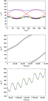 |
Fig. 3 Top panel: evolutionary trajectory of a Type-P particle associated with Set 1 of N-body simulations in the (Ω2, i2) plane (black curve). The initial orbital parameters of this particle are a2 = 20.306 au, e2 = 0.556, i2 = 66.612°, ω2 = 148.109°, and Ω2 = 328.286°. The values of a1 and e1 associated with the inner Jupiter-mass planet, and the red and blue curves are defined in the caption of Fig. 2. The yellow and green circles illustrate the pairs (Ω2, i2) of the particle’s trajectory associated with the vanishing of |


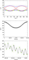 |
Fig. 4 Top panel: trajectory of a Type-P particle associated with Set 1 of N-body simulations in the (Ω2, i2) plane (black curve). The initial orbital parameters of this particle are a2 = 17.424 au, e2 = 0.371, i2 = 69.930°, ω2 = 325.686°, and Ω2 = 159.785°. The values of a1 and e1 associatedwith the inner perturber, and the red and blue curves are defined in the caption of Fig. 2. Middle panel: temporal evolution of the argument of pericenter ω2 of such a particle, which librates by defining an inverse Lidov-Kozai resonance. Bottom panel: zoom of the middle panel between 480 and 600 Myr. The yellow and green circles illustrated in the top and bottom panels are defined in the caption of Fig. 3. |
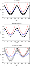 |
Fig. 5 Evolutionary trajectories in the (Ω2, i2) plane of Type-P particles associated with Set 1 of N-body simulations are displayed in a zoom. In every panel, the black curve illustrates the test particle’s trajectory, while the red and blue curves represent the separatrix and the pairs (Ω2, i2) that vanish the ω2 quadrupole precession rate of the system under consideration. The particles illustrated in the top and middle panels are those represented in Figs. 3 and 4, respectively. Bottom panel: initial orbital parameters of the test particle are a2 = 13.833 au, e2 = 0.672, i2 = 63.712°, ω2 = 33.2°, and Ω2 = 138.95°, while the values of a1 and e1 of the inner Jupiter-mass planet are 1.561 au and 0.227, respectively. |
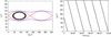 |
Fig. 6 Left panel: trajectory of a Type-F particle corresponding to Set 1 of N-body simulations in the (Ω2, i2) plane (black curve). The initial orbital elements of this particle are a2 = 14.116 au, e2 = 0.262, i2 = 83.136°, ω2 = 156.0°, and Ω2 = 133.263°. The values of a1 and e1 associatedwith the inner perturber, and the red and blue curves are defined in the caption of Fig. 2. Right panel: evolution in time of the argument of pericenter ω2 of the particle. |
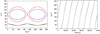 |
Fig. 7 Left panel: trajectory of a Type-P particle associated with Set 3 of N-body simulations in the (Ω2, i2) plane (black curve). The initial orbital elements of this particle are a2 = 38.098 au, e2 = 0.676, i2 = 18.455°, ω2 = 134.168°, and Ω2 = 119.149°. The inner Jupiter-mass planet of such a system has a semimajor axis a1 = 1.778 au and an eccentricity e1 = 0.475. The red curve represents the separatrix of the system, while the blue curve illustrates the pairs (Ω2, i2) that vanish the ω2 quadrupole precession rate for an inner perturber of e1 = 0.475. Right panel: temporal evolution of the argument of pericenter ω2 of the particle. |
4.2 Inner perturber with an eccentricity e1 > e1,F = 0.40825
As we said at the beginning of the present section, the inner massive perturber has an eccentricity e1 greater than e1,F = 0.40825 in nine out of 12 N-body simulations. We also analyze in detail the evolution of the argument of pericenter ω2 of the Type-P, -R, and -F particles associated with the outer small body populations of those resulting systems.
In general terms, the evolution of the argument of pericenter ω2 of the Type-P and -R particles associated with N-body simulations of Set 3 is very simple. In fact, Fig. 7 illustrates the evolution of a given Type-P particle associated with a system with an inner Jupiter-mass planet whose eccentricity e1 is 0.4753. In particular, the left panel exposes the trajectory of such a particle in the (Ω2, i2) plane, which is represented by the black curve. The evolution of such a particle is very similar to that described for the Type-P particle illustrated in Fig. 2. In fact, as the reader can see, the evolutionary trajectory of the particle never crosses the blue curve, which indicates that the ω2 quadrupole precession rate does not vanish. Finally, the right panel of Fig. 7 shows that the argument of pericenter ω2 circulates.
It is worth mentioning that in the nine systems under consideration with an inner massive perturber whose orbit is more eccentric than e1,F = 0.40825, we observe three different kinds of Type-F particles in the resulting outer reservoirs. We note that all Type-F particles produced in our simulations show an orbit-flipping resonance that involves librations of the ascending node longitude Ω2 and variations of the inclination i2 between prograde and retrograde values. The differences observed in those three kinds of Type-F particles are primarily associated with the temporal evolution of the argument of pericenter ω2.
Figure 8 shows the evolution of a Type-F particle representative of the first kind. In particular, the black curve in the left panel illustrates the trajectory of such a particle in the inclination i2 versus ascending node longitude Ω2 plane. While the evolution of the particle is confined to the inner region of the separatrix, it never crosses the blue curve and the ω2 quadrupole precession rate is not vanished for any pair (Ω2, i2) along the entire evolution. The right panel of Fig. 8 shows that the argument of pericenter ω2 of such a Type-F particle evolves in a circulatory regime.
One representative example of a second kind of Type-F particle can be observed in Fig. 9. In particular, the top panel of Fig. 9 describes the evolution of such a particle in the inclination i2 versus ascending node longitude Ω2 plane by a black curve. As the reader can see, the evolutionary trajectory periodically crosses the blue curve, which defines values associated with i2 and Ω2 that vanish the ω2 quadrupole precession rate. For this particular case, the argument of pericenter ω2 circulates reaching local minimum and maximum values, which is illustrated in the middle panel of Fig. 9. As the reader can see, the yellow and green circles, which are associated with the vanishing of  (Eq. (18)) and (dω2∕dτ) (Eq. (24)), respectively, are close and they are in good agreement with the local minimum and maximum values of ω2 observed in the bottom panel of Fig. 9. Moreover, the yellow and green circles are also very close in the (Ω2, i2) plane, which can be seen in the top panel of Fig. 9.
Figure 10 shows the evolution of a Type-F particle representative of the third kind, which is the most interesting one concerning the behavior of the argument of pericenter ω2. In particular, the evolution of such a Type-F particle in the (Ω2, i2) plane is illustrated by a black curve in the top panel of Fig. 10. As in the previous example, the blue curve is periodically crossed by the trajectory associated with the particle, which determines pairs (Ω2, i2) that lead to the vanishing of the ω2 quadrupole precession rate. However, in this particular case, the argument of pericenter ω2 librates around 90° reaching local minimum and maximum values, which can be observed in the temporal evolution of ω2 represented in the middle panel of Fig. 10. From this, the Type-F particles corresponding to this third kind experience an inverse Lidov-Kozai resonance associated with librations of ω2. It is important to remark that these particles are of particular interest since both the ascending node longitude Ω2 as well as the argument of pericenter ω2 evolve in a libration regime, while the inclination i2 oscillates from prograde to retrograde values and back again around 90°.
As in the examples represented in the Figs. 3, 4, and 9, we determine the values of i2, Ω2, and ω2 of the particle’s trajectory associated with the vanishing of  (yellow circles) and (dω2∕dτ) (green circles). On the one hand, according to what is observed in the top panel of Fig. 10, the green and yellow circles are close but they slightly differ from each other in comparison with what is observed in the top panel ofFig. 9, which represents the case of a Type-F particle whose argument of pericenter ω2 circulates. On the other hand, the bottom panel of Fig. 10 shows that the local minimum and maximum values of the temporal evolution of ω2 of a Type-F particle that experiences an inverse Lidov-Kozai resonance are in good agreement with the green circles, while the yellow ones are close.
It is important to describe a peculiar property of the Type-F particles that experience an inverse Lidov-Kozairesonance in comparison with those Type-F particles whose argument of pericenter ω2 circulates. In fact, if ω2 evolves on a circulatory regime, the ascending node longitude Ω2 of the test particle adopts extreme values for orbital inclinations i2 around 90°. Thus, the evolutionary trajectory of such a particle in an inclination i2 versus ascending node longitude Ω2 plane is symmetrical with respect to i2 = 90°. The behavior is very different if the Type-F particle experiences an inverse Lidov-Kozai resonance. In fact, if ω2 evolves on a librating regime, the extreme values of the ascending node longitude Ω2 are not obtained for orbital inclinations i2 around 90°. In such a case, Ω2 adopts extreme values for prograde or retrograde inclinations depending on the center of libration associated with Ω2 and ω2. Thus, the evolutionary trajectory of such a particle in an inclination i2 versus ascending node longitude Ω2 plane shows evidence of an asymmetry with respect to i2 = 90°.
The topic concerning the asymmetrical orbital flips in a (Ω2, i2) plane with respect to i2 = 90° is very interesting. In fact, Zanardi et al. (2018) showed that, when the general relativity is included, the extreme values of the ascending node longitude Ω2 associated with a given outer test particle are obtained for retrograde inclinations, leading to an asymmetrical orbital flip in a (Ω2, i2) plane with respect to i2 = 90°. From this, it is very important to remark that the results derived in the present research indicate that, in the absence of general relativity, the existence of an asymmetrical orbital flip in a (Ω2, i2) plane with respect to an inclination i2 = 90° is a clear sign of an inverse Lidov-Kozai resonance.
We can understand the correlation between the asymmetrical orbital flips and the inverse Lidov-Kozai resonance from analytical considerations. To do this, it is important to remark that it is not enough to analyze the extreme values of the ascending node longitude Ω2 from the vanishing of the Ω2 quadrupole precession rate. In fact, as we mention in Sect. 2, the Ω2 quadrupole precession rate vanishes for an inclination i2 = 90°, which would lead to symmetrical orbital flips in a (Ω2, i2) plane with respect to i2 = 90°, regardless of the evolution of the argument of pericenter ω2. To describe in detail the symmetry or asymmetry of the trajectories associated with Type-F particles in an inclination i2 versus ascending node longitude Ω2 plane with respect to i2 = 90°, we must compute the extreme values of the ascending node longitude Ω2 from the vanishing of the Ω2 precession rate calculated (at least) up to the octupole level of the secular approximation. From Eq. (4) and the expression of the energy function given by Eq. (6), the Ω2 precession rate computed up to the octupole level of the approximation is expressed by
![Mathematical equation: \begin{eqnarray*} \frac{\textrm{d}\Omega_2}{\textrm{d}\tau} &=& -\frac{\partial f_{\text{quad}}}{\partial \theta_2}\frac{1}{J_2}-\frac{\partial f_{\text{oct}}}{\partial \theta_2}\frac{\epsilon}{J_2} \nonumber \\[2pt] &=& \frac{1}{(1-e^2_2)^2}\Bigg\{\alpha\theta_2^2 + \beta\theta_2 + \gamma\Bigg\},\end{eqnarray*}](/articles/aa/full_html/2019/07/aa35220-19/aa35220-19-eq44.png) (26)
(26)
where
![Mathematical equation: \begin{eqnarray*} \alpha &=& \frac{15}{4}e_1\epsilon\Bigg[-45-\frac{15}{2}e^2_1+\frac{105}{2}e^2_1\cos(2\Omega_2)\Bigg]\sin\omega_2\sin\Omega_2, \nonumber \\ \beta &=& -6(2+3e^2_1)+30e^2_1\cos(2\Omega_2) \nonumber \\ &&+\,\frac{15}{4}e_1\epsilon\Bigg[5(2+5e^2_1)-35e^2_1\cos(2\Omega_2)\Bigg]\cos\omega_2\cos\Omega_2, \nonumber \\ \gamma &=& \frac{15}{4}e_1\epsilon\Bigg[11-\frac{e^2_1}{2}-\frac{35}{2}e^2_1\cos(2\Omega_2)\Bigg] \sin\omega_2\sin\Omega_2.\end{eqnarray*}](/articles/aa/full_html/2019/07/aa35220-19/aa35220-19-eq45.png) (27)
(27)
For the particular case of Type-F particles, the ascending node longitude Ω2 evolves in a librating regime. The presence of sines and cosines of the argument of pericenter ω2 in α, β, and γ parameters indicates that the vanishing of the Ω2 precession rate depends on the evolutionary regime associated with ω2.
To understand this, we analyze five Type-F particles of Set 3 of N-body simulations with different modes of behavior concerning the evolution of the argument of pericenter ω2, which are illustrated in Fig. 11. This figure shows five rows, which are numbered from 1 to 5 from top to bottom. Every row refers to a given Type-F particle. The left panels of each row describe the evolution in time of the argument of pericenter ω2 and the ascending node longitude Ω2 of the test particle under study by black and gray curves, respectively. Then, the middle panels represent the evolutionary trajectory in the (Ω2, i2) plane of each Type-F particle by a black curve, while the separatrix and the pairs (Ω2, i2) that vanish the ω2 quadrupole precession rate for the system under consideration are also illustrated by red and blue curves, respectively. Finally, the right panels display a zoom of the middle panels by including the pairs (Ω2, i2) of the trajectory of the corresponding test particle that vanish the Ω2 precession rate computed up to the octupole level of the approximation (Eq. (26)), which are represented by violet circles. Table 1 summarizes the initial orbital parameters associated with the five Type-F particles analyzed in Fig. 11, and the values of the semimajor axis a1 and the eccentricity e1 of the inner Jupiter-mass planet of each system corresponding to such particles.
Row 1 of Fig. 11 illustrates the particular case of a Type-F particle whose argument of pericenter ω2 circulates. According to this, the extreme values of the ascending node longitude Ω2 are obtained for inclinations i2 around 90°, which leads to symmetrical orbital flips in the (Ω2, i2) plane with respect to i2 = 90°.
Row 2 of Fig. 11 describes the evolution of a Type-F particle whose ω2 (Ω2) librates around 90° (270°). From this, the extreme values of Ω2 are associated with retrograde inclinations, which produce asymmetrical orbital flips in the (Ω2, i2) plane with respect to i2 = 90°. This also can be observed in row 3 of Fig. 11. In this case, the particle being studied experiences librations of ω2 (Ω2) around 270° (90°). As in row 2, retrograde inclinations determine the extreme values of Ω2, which leads to an asymmetry in the evolutionary trajectory of the Type-F particle in the (Ω2, i2) plane with respect to i2 = 90°.
Rows 4 and 5 of Fig. 11 show a different result in comparison with that above described. In fact, both the argument of pericenter ω2 as well as the ascending node longitude Ω2 of the Type-F particle analyzed in row 4 (5) librate around 270° (90°). When ω2 and Ω2 have the same center of libration, the extreme values of Ω2 are associated with prograde inclinations, which produces asymmetrical orbital flips in the (Ω2, i2) plane with respect to i2 = 90°.
We would like to remark that the test particle represented in row 4 of Fig. 11 is associated with a system with an inner massive perturber whose eccentricity e1 is of 0.739. This simple example is of significant interest and it illustrates that the inverse Lidov-Kozairesonance can be found even for high values of the inner perturber’s eccentricity e1 from a suitable selection of initial conditions.
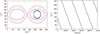 |
Fig. 8 Left panel: evolutionary trajectory of a Type-F particle associated with Set 3 of N-body simulations in the (Ω2, i2) plane (black curve). The initial orbital parameters of this particle are a2 = 23.580 au, e2 = 0.331, i2 = 72.326°, ω2 = 134.249°, and Ω2 = 247.646°. The values of a1 and e1 of the inner Jupiter-mass planet of the system are 1.333 au and 0.566, respectively. The red and blue curves illustrate the separatrix and the pairs (Ω2, i2) that vanish the ω2 quadrupole precession rate for an inner perturber of e1 = 0.566, respectively. Right panel: temporal evolution of the argument of pericenter ω2 of such a particle. |
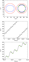 |
Fig. 9 Top panel: trajectory of a Type-F particle associated with Set 3 of N-body simulations in the (Ω2, i2) plane (black curve). The initial orbital parameters of this particle are a2 = 20.332 au, e2 = 0.468, i2 = 56.236°, ω2 = 99.392°, and Ω2 = 233.557°. The values of a1 and e1 associatedwith the inner perturber, and the red and blue curves are defined in the caption of Fig. 8. Middle panel: evolution in time of the argument of pericenter ω2 of such a particle. Bottom panel: zoom of the middle panel between 20 and 50 Myr. The references associated with the yellow and green circles illustrated in the top and bottom panels are described in the caption of Fig. 3. |
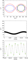 |
Fig. 10 Top panel: evolutionary trajectory of a Type-F particle associated with Set 3 of N-body simulations in the (Ω2, i2) plane (black curve). The initial orbital parameters of this particle are a2 = 34.201 au, e2 = 0.696, i2 = 52.853°, ω2 = 120.147°, and Ω2 = 254.671°. The values of a1 and e1 associatedwith the inner perturber, and the red and blue curves are defined in the caption of Fig. 7. Middle panel: evolution in time of the argument of pericenter ω2 of such a particle, which librates around 90° by defining an inverse Lidov-Kozai resonance. Bottom panel: zoom of the middle panel between 1.44 and 1.52 Gyr. The references associated with the yellow and green circles represented in the top and bottom panels are described in the caption of Fig. 3. |
5 Discussion and conclusions
In the present research, we study the evolution of the argument of pericenter ω2 of outer test particles that orbit a given central star and undergo the effects of an inner massive perturber. In particular, we describe the behavior of ω2 as a function of the orbital eccentricity e1 of the inner perturber. The key result derived in our study indicates that the inverse Lidov-Kozai or ω2 resonance can appear for small, moderate, and high values of e1 as long as suitable initial conditions mainly associated with i2 and Ω2 are adopted.
First, we carried out our investigation from analytical considerations. To do this, we adopted the expression of the potential expanded up to the octupole level of the secular approximation derived by Naoz et al. (2017), as well as the term of hexadecapolar order included later by Vinson & Chiang (2018). From this, we computed equations that express the contributionof the terms of quadrupole, octupole, and hexadecapolar order of the secular approximation to the ω2 precession rate. Our study suggests that the pairs (Ω2, i2) that vanish the ω2 quadrupole precession rate  strongly depend on the eccentricity e1 of the inner perturber. In fact, if e1 < 0.25,
  is only vanished for test particles on prograde and retrograde orbits whose ascending node longitude Ω2 evolves in a circulatory regime, while, if e1 > 0.40825,
  is only vanished for test particles that experience an orbit-flipping resonance, in which Ω2 librates. For inner perturber eccentricities e1 between 0.25 and 0.40825, our analysis indicates that any test particle can vanish the ω2 quadrupole precession rate regardless of the evolutionary regime of the ascending node longitude Ω2, for pairs (Ω2, i2) that satisfy the relation given by Eq. (25).
Furthermore, we used the analytical considerations derived in our research with the aim of describing the behavior of test particles, which result from a set of N-body simulations presented by Zanardi et al. (2017). On the basis of such simulations, we analyzed the evolution of the argument of pericenter ω2 of outer test particles that evolve under the effects of a Jupiter-mass planet around a 0.5 M⊙ star. The eccentricity e1 of the inner perturber associated with the sample of simulations of work ranges from 0.227 to 0.94. We remark that the evolution of ω2 of the outer test particles extracted from the N-body simulations carried out by Zanardi et al. (2017) is in very good agreement with the analytical criteria derived in the present investigation.
It is very important to mention that, unlike the results proposed by Vinson & Chiang (2018), who found the inverse Lidov-Kozai resonance only up to e1 = 0.1 in N-body experiments, we observed outer test particles that experience a ω2 resonance for an inner perturber’s eccentricity e1 as high as 0.8 in the N-body simulations that represent our frame of work. As we remarked at the beginning of this section, our research indicates that the inverse Lidov-Kozai resonance can be found even for high values of e1 as long as a correct choice of the initial conditions is made.
It is worth noting that the inverse Lidov-Kozai resonance produces some distinctive features in the evolution of a test particle in the inclination i2 versus ascending node longitude Ω2 plane. On the one hand, if a given particle experiences an inverse Lidov-Kozai resonance and its ascending node longitude Ω2 evolves in a circulatory regime, the extreme values of the inclination i2 at Ω2 = 90° and 270° are not equal. Our study shows that the value of Ω2 associated with the absolute extreme of i2 depends on the center of libration of ω2. On the other hand, if a test particle is in an inverse Lidov-Kozai resonance and its ascending node longitude Ω2 librates, the evolutionary trajectory of such a particle in the inclination i2 versus ascending node longitude Ω2 plane shows evidence of an asymmetry with respect to i2 = 90°. Our analysis shows that the extreme values of Ω2 are obtainedfor values of i2 less or higher than 90°, which depends on the centers of libration associated with Ω2 and ω2. We remark that such distinctive features observed in the evolution of test particles extracted from the N-body experiments are very well described from the analytical expressions derived in our investigation.
It is important to mention that our investigation shows that the vanishing of ω2 quadrupole precession rate is not a sufficient condition for the inverse Lidov-Kozai resonance. A more detailed study is beyond the scope of this paper.
The dynamics discussed in this research could play a key role in understanding the evolution of debris disks associated with extrasolar systems that host an inner and eccentric giant planet. In this sense, planetary systems such as HD 10647, HD 39091, HD 50499, HD 50554, and HD 210277 can serve as valuable laboratories to contrast theoretical results with observational evidence from dynamical and collisional models associated with the evolution of debris disks.
The present work represents a detailed investigation that combines analytical considerations and numerical results derived from N-body simulations concerning the inverse Lidov-Kozai resonance. Such a treatment allows us to obtain a better understanding of the evolution of the argument of pericenter ω2 of an outer test particle in the elliptical restricted three-body problem.
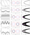 |
Fig. 11 Evolution of different Type-F particles associated with Set 3 of N-body simulations. The rows are numbered from 1 to 5 from top to bottom. In every row, the black and gray curves of the left panel illustrate the evolution in time of ω2 and Ω2, respectively. Then, the black and red curves of the middle panel represent the trajectory of the particle and the separatrix in the plane (Ω2, i2), respectively, while the blue curve shows the pairs (Ω2, i2) of the particle’s trajectory that vanish the ω2 quadrupole precession rate of the system under consideration. Finally, the violet circles of the right panel illustrate the pairs (Ω2, i2) of the particle’s trajectory that vanish the Ω2 precession rate calculated up to the octupole level of the approximation. The initial orbital parameters of the test particles and the values of a1 and e1 associated with the inner Jupiter-mass planet are specified for every row in Table 1. |
Initial orbital parameters.
Acknowledgements
This work was partially financed by CONICET through PIP 0436/13, and Agencia de Promoción Científica, through PICT 2014-1292 and PICT 201-0505. We thank the anonymous referee for valuable suggestions, which helped us to improve the manuscript. Moreover, G.C.dE, M.Z., and A.D. acknowledge the financial support by FCAGLP and IALP for extensive use of their computing facilities, and S.N. acknowledges the partial support from the NSF through Grant No. AST-173916. Finally, G.C.dE and M.Z. wish to dedicate the present paper to the memory of Carlos Rafael de Elía.
References
- Chambers, J. E. 1999, MNRAS, 304, 793 [NASA ADS] [CrossRef] [MathSciNet] [Google Scholar]
- Everhart, E. 1985, in Dynamics of Comets: Their Origin and Evolution, Proceedings of IAU Colloq. 83, held in Rome, Italy, June 11–15, 1984, eds. A. Carusi & G. B. Valsecchi (Dordrecht: Reidel) Astrophys. Space Sci. Lib., 115, 185 [NASA ADS] [CrossRef] [Google Scholar]
- Farago, F., & Laskar, J. 2010, MNRAS, 401, 1189 [NASA ADS] [CrossRef] [Google Scholar]
- Ford, E. B., Kozinsky, B., & Rasio, F. A. 2000, ApJ, 535, 385 [NASA ADS] [CrossRef] [Google Scholar]
- Gallardo, T., Hugo, G., & Pais, P. 2012, Icarus, 220, 392 [NASA ADS] [CrossRef] [Google Scholar]
- Harrington, R. S. 1968, AJ, 73, 190 [NASA ADS] [CrossRef] [Google Scholar]
- Katz, B., Dong, S., & Malhotra, R. 2011, Phys. Rev. Lett., 107, 181101 [NASA ADS] [CrossRef] [Google Scholar]
- Kozai, Y. 1962, AJ, 67, 591 [Google Scholar]
- Krymolowski, Y., & Mazeh, T. 1999, MNRAS, 304, 720 [NASA ADS] [CrossRef] [Google Scholar]
- Li, D., Zhou, J.-L., & Zhang, H. 2014, MNRAS, 437, 3832 [NASA ADS] [CrossRef] [Google Scholar]
- Lidov, M. L. 1962, Planet. Space Sci., 9, 719 [NASA ADS] [CrossRef] [Google Scholar]
- Lithwick, Y., & Naoz, S. 2011, ApJ, 742, 94 [NASA ADS] [CrossRef] [Google Scholar]
- Naoz, S., Farr,W. M., Lithwick, Y., Rasio, F. A., & Teyssandier, J. 2013, MNRAS, 431, 2155 [NASA ADS] [CrossRef] [Google Scholar]
- Naoz, S., Li, G., Zanardi, M., de Elía, G. C., & Di Sisto, R. P. 2017, AJ, 154, 18 [NASA ADS] [CrossRef] [Google Scholar]
- Soderhjelm, S. 1984, A&A, 141, 232 [NASA ADS] [Google Scholar]
- Vinson, B. R., & Chiang, E. 2018, MNRAS, 474, 4855 [NASA ADS] [CrossRef] [Google Scholar]
- Yokoyama, T., Santos, M. T., Cardin, G., & Winter, O. C. 2003, A&A, 401, 763 [NASA ADS] [CrossRef] [EDP Sciences] [Google Scholar]
- Zanardi, M., de Elía, G. C., Di Sisto, R. P., et al. 2017, A&A, 605, A64 [NASA ADS] [CrossRef] [EDP Sciences] [Google Scholar]
- Zanardi, M., de Elía, G. C., Di Sisto, R. P., & Naoz, S. 2018, A&A, 615, A21 [NASA ADS] [CrossRef] [EDP Sciences] [Google Scholar]
- Ziglin, S. L. 1975, Sov. Astron. Lett., 1, 194 [NASA ADS] [Google Scholar]
We define flipped orbits as those whose inclination i oscillates from below 90° to above 90°. In other words, our definition focuses on the i = 90° transition rather than the location and phase of i in the surface of section.
We note that Naoz et al. (2017) had a typographical error in their Eq. (7) concerning foct, which should have been preceded with a minus sign. It is worth noting that the equations of motion were calculated using the correct hamiltonian.
It is important to remark that the terms of the energy function derived by Vinson & Chiang (2018) differ from those obtained by Naoz et al. (2017) in a constant factor. In particular, if we compare the quadrupole terms proposed in both works, it is possible to observe that the quadrupole term from Naoz et al. (2017) is obtained dividing the quadrupole term from Vinson & Chiang (2018) by
 . Thus, we divide by such a factor the hexadecapolar term from Vinson & Chiang (2018) given by c3 Rhex in order to use the equations of motion derived by Naoz et al. (2017) with the aim of calculating the hexadecapolar contribution of the secular approximation to the ω2 precession rate.
Zanardi et al. (2017) carried out the N-body simulations using the MERCURY code (Chambers 1999). In particular, the authors used the RA15 version of the RADAU numerical integrator with an accuracy parameter of 10−12 (Everhart 1985).
All Tables
All Figures
|
Fig. 1 Pairs (Ω2, i2) that vanish the ω2 quadrupole precession rate are illustrated by a blue curve for different values of the eccentricity e1 associated with the inner perturber, which is specified at the top left corner of every panel. For each scenario, the separatrix of the system, which is computed up to the quadruple level of the secular approximation, is represented by a red curve, while the red shaded region illustrates the pairs (Ω2, i2) that lead to the orbit-flipping quadrupole resonance. |
| In the text | |
|
Fig. 2 Left panel: evolutionary trajectory of a Type-P particle associated with the Set 1 of N-body simulations is represented by the black curve in an inclination i2 versus ascending node longitude Ω2 plane. The initial orbital elements of this particle are a2 = 21.935 au, e2 = 0.452, i2 = 37.129°, ω2 = 165.966°, and Ω2 = 97.285°. The inner Jupiter-mass planet of such a system has a semimajor axis a1 = 1.011 au and an eccentricity e1 = 0.237. The red curve represents the separatrix of the system, while the blue curve illustrates the pairs (Ω2, i2) that vanish the ω2 quadrupole precession rate for an inner perturber of e1 = 0.237. Right panel: temporal evolution of the argument of pericenter ω2 of the same particle. |
| In the text | |
|
Fig. 3 Top panel: evolutionary trajectory of a Type-P particle associated with Set 1 of N-body simulations in the (Ω2, i2) plane (black curve). The initial orbital parameters of this particle are a2 = 20.306 au, e2 = 0.556, i2 = 66.612°, ω2 = 148.109°, and Ω2 = 328.286°. The values of a1 and e1 associated with the inner Jupiter-mass planet, and the red and blue curves are defined in the caption of Fig. 2. The yellow and green circles illustrate the pairs (Ω2, i2) of the particle’s trajectory associated with the vanishing of |
| In the text | |
|
Fig. 4 Top panel: trajectory of a Type-P particle associated with Set 1 of N-body simulations in the (Ω2, i2) plane (black curve). The initial orbital parameters of this particle are a2 = 17.424 au, e2 = 0.371, i2 = 69.930°, ω2 = 325.686°, and Ω2 = 159.785°. The values of a1 and e1 associatedwith the inner perturber, and the red and blue curves are defined in the caption of Fig. 2. Middle panel: temporal evolution of the argument of pericenter ω2 of such a particle, which librates by defining an inverse Lidov-Kozai resonance. Bottom panel: zoom of the middle panel between 480 and 600 Myr. The yellow and green circles illustrated in the top and bottom panels are defined in the caption of Fig. 3. |
| In the text | |
|
Fig. 5 Evolutionary trajectories in the (Ω2, i2) plane of Type-P particles associated with Set 1 of N-body simulations are displayed in a zoom. In every panel, the black curve illustrates the test particle’s trajectory, while the red and blue curves represent the separatrix and the pairs (Ω2, i2) that vanish the ω2 quadrupole precession rate of the system under consideration. The particles illustrated in the top and middle panels are those represented in Figs. 3 and 4, respectively. Bottom panel: initial orbital parameters of the test particle are a2 = 13.833 au, e2 = 0.672, i2 = 63.712°, ω2 = 33.2°, and Ω2 = 138.95°, while the values of a1 and e1 of the inner Jupiter-mass planet are 1.561 au and 0.227, respectively. |
| In the text | |
|
Fig. 6 Left panel: trajectory of a Type-F particle corresponding to Set 1 of N-body simulations in the (Ω2, i2) plane (black curve). The initial orbital elements of this particle are a2 = 14.116 au, e2 = 0.262, i2 = 83.136°, ω2 = 156.0°, and Ω2 = 133.263°. The values of a1 and e1 associatedwith the inner perturber, and the red and blue curves are defined in the caption of Fig. 2. Right panel: evolution in time of the argument of pericenter ω2 of the particle. |
| In the text | |
|
Fig. 7 Left panel: trajectory of a Type-P particle associated with Set 3 of N-body simulations in the (Ω2, i2) plane (black curve). The initial orbital elements of this particle are a2 = 38.098 au, e2 = 0.676, i2 = 18.455°, ω2 = 134.168°, and Ω2 = 119.149°. The inner Jupiter-mass planet of such a system has a semimajor axis a1 = 1.778 au and an eccentricity e1 = 0.475. The red curve represents the separatrix of the system, while the blue curve illustrates the pairs (Ω2, i2) that vanish the ω2 quadrupole precession rate for an inner perturber of e1 = 0.475. Right panel: temporal evolution of the argument of pericenter ω2 of the particle. |
| In the text | |
|
Fig. 8 Left panel: evolutionary trajectory of a Type-F particle associated with Set 3 of N-body simulations in the (Ω2, i2) plane (black curve). The initial orbital parameters of this particle are a2 = 23.580 au, e2 = 0.331, i2 = 72.326°, ω2 = 134.249°, and Ω2 = 247.646°. The values of a1 and e1 of the inner Jupiter-mass planet of the system are 1.333 au and 0.566, respectively. The red and blue curves illustrate the separatrix and the pairs (Ω2, i2) that vanish the ω2 quadrupole precession rate for an inner perturber of e1 = 0.566, respectively. Right panel: temporal evolution of the argument of pericenter ω2 of such a particle. |
| In the text | |
|
Fig. 9 Top panel: trajectory of a Type-F particle associated with Set 3 of N-body simulations in the (Ω2, i2) plane (black curve). The initial orbital parameters of this particle are a2 = 20.332 au, e2 = 0.468, i2 = 56.236°, ω2 = 99.392°, and Ω2 = 233.557°. The values of a1 and e1 associatedwith the inner perturber, and the red and blue curves are defined in the caption of Fig. 8. Middle panel: evolution in time of the argument of pericenter ω2 of such a particle. Bottom panel: zoom of the middle panel between 20 and 50 Myr. The references associated with the yellow and green circles illustrated in the top and bottom panels are described in the caption of Fig. 3. |
| In the text | |
|
Fig. 10 Top panel: evolutionary trajectory of a Type-F particle associated with Set 3 of N-body simulations in the (Ω2, i2) plane (black curve). The initial orbital parameters of this particle are a2 = 34.201 au, e2 = 0.696, i2 = 52.853°, ω2 = 120.147°, and Ω2 = 254.671°. The values of a1 and e1 associatedwith the inner perturber, and the red and blue curves are defined in the caption of Fig. 7. Middle panel: evolution in time of the argument of pericenter ω2 of such a particle, which librates around 90° by defining an inverse Lidov-Kozai resonance. Bottom panel: zoom of the middle panel between 1.44 and 1.52 Gyr. The references associated with the yellow and green circles represented in the top and bottom panels are described in the caption of Fig. 3. |
| In the text | |
|
Fig. 11 Evolution of different Type-F particles associated with Set 3 of N-body simulations. The rows are numbered from 1 to 5 from top to bottom. In every row, the black and gray curves of the left panel illustrate the evolution in time of ω2 and Ω2, respectively. Then, the black and red curves of the middle panel represent the trajectory of the particle and the separatrix in the plane (Ω2, i2), respectively, while the blue curve shows the pairs (Ω2, i2) of the particle’s trajectory that vanish the ω2 quadrupole precession rate of the system under consideration. Finally, the violet circles of the right panel illustrate the pairs (Ω2, i2) of the particle’s trajectory that vanish the Ω2 precession rate calculated up to the octupole level of the approximation. The initial orbital parameters of the test particles and the values of a1 and e1 associated with the inner Jupiter-mass planet are specified for every row in Table 1. |
| In the text | |
Current usage metrics show cumulative count of Article Views (full-text article views including HTML views, PDF and ePub downloads, according to the available data) and Abstracts Views on Vision4Press platform.
Data correspond to usage on the plateform after 2015. The current usage metrics is available 48-96 hours after online publication and is updated daily on week days.
Initial download of the metrics may take a while.