| Issue |
A&A
Volume 689, September 2024
|
|
|---|---|---|
| Article Number | A99 | |
| Number of page(s) | 12 | |
| Section | Celestial mechanics and astrometry | |
| DOI | https://doi.org/10.1051/0004-6361/202450912 | |
| Published online | 06 September 2024 | |
Von Zeipel-Lidov-Kozai secondary resonances can enhance the excitation of planetary eccentricity
1
School of Astronomy and Space Science, Nanjing University,
Nanjing
210023,
China
2
Key Laboratory of Modern Astronomy and Astrophysics in Ministry of Education, Nanjing University,
Nanjing
210023,
China
Received:
29
May
2024
Accepted:
28
June
2024
Abstract
The von Zeipel-Lidov-Kozai (ZLK) effect has been applied to a wide range of dynamical circumstances, covering satellites and planets to supermassive black holes, in order to explain physical phenomena. The evolution of periodic orbit families associated with ZLK resonance under the octupole-level approximation exhibits distinctly different dynamical structures from the standard ZLK effect. In particular, bifurcations of periodic-orbit families commonly exist in planetary systems with a wide range of mass ratios. It is shown that such a phenomenon of bifurcation is triggered by ZLK secondary resonance, which is a new dynamical mechanism that has not appeared in previous studies. Numerical analysis shows that ZLK secondary resonance leads to a stronger excitation of eccentricity and/or inclination than the standard ZLK effect and that the level of enhancement is dependent on the initial eccentricity. The technique of perturbative treatments is adopted to study dynamical structures of ZLK secondary resonances, showing that there is an excellent agreement between analytical structures arising in phase portraits and numerical structures arising in Poincaré sections. Phase-space structures are produced for actual exoplanetary systems including HAT-P-11, HAT-P-13, and HAT-P-44, where large excitation of planetary eccentricity and/or inclination is expected due to the emergence of ZLK secondary resonance.
Key words: methods: miscellaneous / celestial mechanics / planets and satellites: dynamical evolution and stability
Corresponding author; This email address is being protected from spambots. You need JavaScript enabled to view it.
© The Authors 2024
 Open Access article, published by EDP Sciences, under the terms of the Creative Commons Attribution License (https://creativecommons.org/licenses/by/4.0), which permits unrestricted use, distribution, and reproduction in any medium, provided the original work is properly cited.
This article is published in open access under the Subscribe to Open model. This email address is being protected from spambots. You need JavaScript enabled to view it. to support open access publication.
1 Introduction
The hierarchical three-body problem is a basic dynamical model that describes a binary system perturbed by a third body situated at a considerable distance. This configuration gives rise to diverse captivating dynamical phenomena. In this regard, Kozai (1962) and Lidov (1962) independently discovered the coupled oscillations between eccentricity and inclination when the mutual inclination is between 39.2° and 140.8°, under the configuration where the perturber is moving on a circular orbit. Recently, it was pointed out that von Zeipel (1910) also conducted a similar analysis before Lidov and Kozai (Ito & Ohtsuka 2019). Thus, the suggested name for such a coupled oscillation between eccentricity and inclination due to an inclined third-body perturbation at the quadrupole-order approximation is the von Zeipel-Lidov-Kozai (ZLK) effect (Ito & Ohtsuka 2019).
When the third body moves on an inclined and eccentric orbit, the secular approximation should be truncated up to the octupole order in semimajor axis ratio. Under this model, a flip of inclination from prograde to retrograde may occur in the long-term evolution, accompanying an excited eccentricity close to one. This phenomenon is attributed to the eccentric ZLK effect (Naoz 2016). Due to the eccentric ZLK effect, Lithwick & Naoz (2011) pointed out that orbit flipping is a very common phenomenon if the eccentricity of the third body is high enough. In particular, configurations of orbit flipping are usually classified into two categories (Li et al. 2014a): the low-eccentricity, high-inclination (LeHi) and the high-eccentricity, low-inclination (HeLi) cases. Their underlying mechanisms are different: the LeHi type of flip is attributed to the combination of quadrupole-order and octupole-order effects, while the HeLi type of flip is caused by the octupole-order effect (Li et al. 2014a,b). Other parameters, such as the semimajor axis and mass ratio of the outer to the inner planet, may also have influences on the conditions of orbit flips (Teyssandier et al. 2013; Hansen & Naoz 2020; Huang & Lei 2024). Regarding orbit flipping caused by the eccentric ZLK effect, Sidorenko (2018) interpreted it as a resonance phenomenon. Under non-restricted hierarchical planetary systems, Lei & Huang (2022) and Huang & Lei (2022) explored the eccentric ZLK effect from the viewpoint of perturbative treatments at the octupole-level approximation and they pointed out that orbit flipping caused by an eccentric ZLK effect is induced by the octupole-order resonance (i.e., the apsidal resonance). Under restricted hierarchical planetary systems, an intrinsic connection between the phenomenon of orbit flipping and the octupole-order resonance is illustrated by Lei & Gong (2022) and Lei (2022).
The (eccentric) ZLK effect can help us to understand the pathway of occurrence for high-eccentricity and/or high-inclination exoplanets (Takeda & Rasio 2005). In particular, its combination with tidal friction offers a highly reliable mechanism for producing hot Jupiter on highly misaligned orbits (Fabrycky & Tremaine 2007; Naoz et al. 2011, 2012; Petrovich 2015; Dawson & Johnson 2018). In this regard, Beust et al. (2012) proposed that GJ 436b was formerly located far away from the central star and then experienced a migration induced by the combined effect of third-body perturbation and tidal friction. The effective excitation of eccentricity can enhance the efficiency of gravitational-wave radiation, resulting in the acceleration of merger events. Thus, it provides a pathway for the formation and merger of compact binary stars (Thompson 2011) and binary black holes (Blaes et al. 2002; Safarzadeh et al. 2020; Fragione & Antonini 2019). In addition, the eccentric ZLK can enhance the idal disruption of stars around the supermassive black hole at the center of a galaxy (Wegg & Bode 2011). Additional applications can be observed in main-belt asteroids (Kozai 1962), near-Earth asteroids (Michel & Thomas 1996), Kuiper asteroids (Bailey et al. 1992), binary minor planets (Naoz et al. 2010), and disk dynamics (Subr & Karas 2005; Zhao et al. 2012; Martin et al. 2014).
Recently, Huang & Lei (2024) investigated the influences of mass ratio on dynamical structures under non-restricted hierarchical three-body systems. An unexpected observation is the emergence of bifurcation in the evolution of periodic-orbit families associated with ZLK resonance under the octupole-level Hamiltonian model. Such a bifurcation phenomenon inside a ZLK resonant region is new and its dynamical effects are not clear. In this work, we aim to conduct a comprehensive study about this bifurcation phenomenon. The purpose of this study is twofold. First, we explored the influence of the bifurcation phenomenon on the excitation of eccentricity and/or inclination under the octupole-order Hamiltonian model. Second, we clarified the underlying dynamical mechanism causing bifurcation phenomena inside the ZLK resonance.
This paper is organized as follows. In Sec. 2, we describe a phase-averaged Hamiltonian model formulated up to the octupole order in semimajor axis ratio. In Sec. 3, we discuss the numerical exploration performed with regard to the bifurcation phenomenon inside the ZLK resonance. The dynamics of ZLK secondary resonances was analytically studied by taking advantage of perturbation theory, which we outline in Sec. 4, and applications of analytical solutions to three exoplanet systems are discussed in Sec. 5. Finally, the conclusion is summarized in Sec. 6.
2 Hamiltonian model
A hierarchical three-body planetary system consists of a central star with a mass of m0, an inner planet with a mass of m1, and an outer planet with a mass of m2. The central star and the inner planet form an inner binary system; the outer planet is located at a greater distance. Usually, the dynamical model is formulated under an m0-centered inertial coordinate system, where the x-y plane is taken as the invariant plane of the system, the x-axis is along the nodal line, the z-axis points toward the direction of the total angular momentum vector, and the right-handed rule determines the direction of the y-axis. Under such a defined inertial frame, Jacobi coordinates are introduced. For convenience, orbits of the inner and outer planets are characterized by orbital elements: the semimajor axis a1,2, eccentricity e1,2, inclination i1,2, longitude of the ascending node Ω1,2, argument of pericenter ω1,2, and mean anomaly M1,2. The mutual inclination is denoted by itot = i1 + i2. Unless stated otherwise, we used subscript 1 to denote the inner planet and subscript 2 for the outer planet.
We denote the ratio of semimajor axes as α, which is a small parameter for a hierarchical three-body configuration. As a result, it is possible to perform a Legendre expansion for the disturbing function, which is a power series in terms of α (Harrington 1968, 1969). The Hamiltonian truncated at the second order in α is usually referred to as the quadrupole-level truncation, and the one up to the third order in α is known as the octupole-level approximation. In order to study the long-term evolution, it is common to remove those short-period effects by performing double averages over the orbital periods of the inner and outer planets (phase-averaged), leading to the double-averaged Hamiltonian function. A similar secular approximation can be found in Lei (2020) and Lei et al. (2022) for studying the long-term dynamics of navigation satellites. In particular, the secular approximation up to the octupole order in α reads (Krymolowski & Mazeh 1999; Ford et al. 2000; Blaes et al. 2002; Naoz et al. 2013; Naoz 2016)
![Mathematical equation: $\[\mathcal{H}=-C_0\left(\mathcal{H}_2+\varepsilon \mathcal{H}_3\right),\]$](/articles/aa/full_html/2024/09/aa50912-24/aa50912-24-eq1.png) (1)
(1)
where the parameters C0 and ϵ are given by
![Mathematical equation: $\[C_0=\frac{\mathcal{G} m_0 m_1 m_2}{16\left(m_0+m_1\right)} \frac{a_1^2}{a_2^3}, \quad \varepsilon=\frac{m_0-m_1}{m_0+m_1} \frac{a_1}{a_2},\]$](/articles/aa/full_html/2024/09/aa50912-24/aa50912-24-eq2.png) (2)
(2)
with ![Mathematical equation: $\[\mathcal{G}\]$](/articles/aa/full_html/2024/09/aa50912-24/aa50912-24-eq3.png) being the universal gravitational constant. In Eq. (1), ℋ2 and ℋ3 are the quadrupole- and octupole-order Hamiltonian terms, given by
being the universal gravitational constant. In Eq. (1), ℋ2 and ℋ3 are the quadrupole- and octupole-order Hamiltonian terms, given by
![Mathematical equation: $\[\begin{aligned}\mathcal{H}_2= & \frac{1}{\left(1-e_2^2\right)^{3 / 2}}\left[\left(2+3 e_1^2\right)\left(3 \cos ^2 i_{\text {tot }}-1\right)\right. \\& \left.+15 e_1^2\left(1-\cos ^2 i_{\text {tot }}\right) \cos ~(2 \omega_1)\right]\end{aligned}\]$](/articles/aa/full_html/2024/09/aa50912-24/aa50912-24-eq4.png)
and
![Mathematical equation: $\[\begin{aligned}\mathcal{H}_3= & \frac{15}{32} \frac{e_1 e_2}{\left(1-e_2^2\right)^{5 / 2}}\left\{\left(4+3 e_1^2\right)\right. \\& {\left[\left(-1+11 \cos i_{\mathrm{tot}}+5 \cos ^2 i_{\mathrm{tot}}-15 \cos ^3 i_{\mathrm{tot}}\right) \cos ~\left(\omega_1+\omega_2\right)\right.} \\& \left.+\left(-1-11 \cos i_{\mathrm{tot}}+5 \cos ^2 i_{\mathrm{tot}}+15 \cos ^3 i_{\mathrm{tot}}\right) \cos ~\left(\omega_1-\omega_2\right)\right] \\& +35 e_1^2\left[\left(1-\cos i_{\mathrm{tot}}-\cos ^2 i_{\mathrm{tot}}+\cos ^3 i_{\mathrm{tot}}\right) \cos ~\left(3 \omega_1+\omega_2\right)\right. \\& \left.\left.+\left(1+\cos i_{\mathrm{tot}}-\cos ^2 i_{\mathrm{tot}}-\cos ^3 i_{\mathrm{tot}}\right) \cos ~\left(3 \omega_1-\omega_2\right)\right]\right\}.\end{aligned}\]$](/articles/aa/full_html/2024/09/aa50912-24/aa50912-24-eq5.png)
Under the phase-averaged model, it is evident that mean anomalies M1 and M2 are cyclic variables in the octupole-level Hamiltonian; thus, their conjugate momenta are integral of motion, showing that a1 and a2 remain unchanged during the long-term evolution. As a result, the coefficient C0 is a constant under the phase-averaged Hamiltonian model. For convenience, the Hamiltonian function can be normalized by C0 (Lei & Huang 2022; Huang & Lei 2022).
Similarly to previous studies (Huang & Lei 2022; Lei & Huang 2022), we introduce a set of normalized Delaunay’s variables:
![Mathematical equation: $\[\begin{array}{ll}g_1=\omega_1, & G_1=\sqrt{1-e_1^2}, \\g_2=\omega_2, & G_2=\beta \sqrt{1-e_2^2}, \\h_1=\Omega_1, & H_1=G_1 \cos i_1, \\h_2=\Omega_2, & H_2=G_2 \cos i_2,\end{array}\]$](/articles/aa/full_html/2024/09/aa50912-24/aa50912-24-eq6.png)
where G1 and G2 correspond to the (normalized) angular momentum of inner and outer orbits, respectively, and β is a constant, given by
![Mathematical equation: $\[\beta=G_2 / G_1=\frac{\left(m_0+m_1\right) m_2}{m_0 m_1} \sqrt{\frac{m_0+m_1}{m_0+m_1+m_2} \frac{a_2}{a_1}},\]$](/articles/aa/full_html/2024/09/aa50912-24/aa50912-24-eq7.png)
measuring the ratio of angular momenta of the inner and outer planets moving on circular orbits. The total angular-momentum magnitude is designated as Gtot = G1 cos i1 + G2 cos i2 (Naoz et al. 2013). Hence, the relationship between Gtot and itot is given by
![Mathematical equation: $\[\cos i_{\text {tot }}=\frac{G_{\mathrm{tot}}^2-G_1^2-G_2^2}{2 G_1 G_2}.\]$](/articles/aa/full_html/2024/09/aa50912-24/aa50912-24-eq8.png) (3)
(3)
Additionally, the equations of motion can be obtained through Hamiltonian canonical relations (Morbidelli 2002):
![Mathematical equation: $\[\frac{\mathrm{d} g_j}{\mathrm{~d} \tau}=\frac{\partial \mathcal{H}}{\partial G_j}, \quad \frac{\mathrm{d} G_j}{\mathrm{~d} \tau}=-\frac{\partial \mathcal{H}}{\partial g_j}\]$](/articles/aa/full_html/2024/09/aa50912-24/aa50912-24-eq9.png)
with j = 1, 2. Therefore, we can see that the Hamiltonian represented by Equation (1) determines a two-degrees-of-freedom (2-DOF) dynamical model, depending on the total angular momentum Gtot.
Unless stated otherwise, the parameters adopted in the work are the same as the ones adopted by Huang & Lei (2024). The mass of the central object m0 is fixed as the solar mass (i.e., m0 = 1.0 mS), the mass of the inner planet is taken as the Jovian mass (i.e., m1 = 1.0 mJ), and the semimajor axis is fixed at a1 = 1.298 au for the inner planet and a2 = 23.72618 au for the outer planet. Physical data of the example planetary system come from Tamuz et al. (2008) and Cheetham et al. (2017). The mass of the outer planet m2 is limited to the [1.1 mJ, 40 mJ] range. The total angular momentum is a conserved quantity of the system, and it can be characterized in the following form (Lei & Huang 2022):
![Mathematical equation: $\[G_{\mathrm{tot}}=\sqrt{\left(1+\beta^2\right)\left(1-0.3^2\right)},\]$](/articles/aa/full_html/2024/09/aa50912-24/aa50912-24-eq10.png)
which corresponds to the initial eccentricities of the inner and outer planets at e1,0 = e2,0 = 0.3 and the initial mutual inclination at itot = 90°. We can see that the magnitude of Gtot is uniquely determined by β. It is known that the parameter β is uniquely determined by m2 if m1 is fixed. As a result, Gtot is uniquely determined by the mass ratio αm = m2/m1 (m1 is fixed at m1 = 1.0 mJ). Additionally, considering the fact that the bifurcation only appears in the prograde space, we limited our study to the space with itot < 90°.
3 Numerical explorations
In this section, dynamical structures inside ZLK resonance at the octupole-order approximation is studied by taking advantage of numerical methods. In particular, dynamical system approaches including the Poincaré section technique and the periodic-orbit method are utilized to reveal numerical structures in phase space and, finally, the influence of the bifurcation phenomenon on eccentricity excitation is discussed.
3.1 Poincaré sections
As the current octupole-order Hamiltonian model is of two degrees of freedom, it is convenient for us to preliminarily explore the phase-space structures by analyzing Poincaré sections (Li et al. 2014a; Lei 2022). Usually, the smooth curves arising in the section stand for regular (quasi-periodic) orbits, the center of an island stands for a stable periodic orbit, and 2D scattered points show that these regions are full of chaotic orbits. The Poincaré section technique provides a powerful tool for exploring dynamical structures in the entire phase space.
As the focus of this work is to study dynamical structures inside the ZLK resonance in the (g1, G1) space, we define the Poincaré section by
![Mathematical equation: $\[g_2=\pi / 2, \quad \dot{g}_2>0 .\]$](/articles/aa/full_html/2024/09/aa50912-24/aa50912-24-eq11.png) (4)
(4)
The states of planets are recorded every time when they cross the defined section. Considering the fact that g2 is circulating for all the motions inside ZLK resonance (this can be verified by performing numerical simulations), we could take the arbitrary value of g2 to define the section (i.e., taking a snapshot for the Hamiltonian flow).
It should be mentioned that the current 2-DOF Hamiltonian is determined by a given total angular momentum Gtot, which is uniquely characterized by the mass ratio αm (see Sect. 1 for discussions). In practice, we take αm = 1.1 to represent the case of a low mass ratio and αm = 40 to represent the case of a high mass ratio. Their respective Poincaré sections are presented in Figs. 1 and 2. In each case, intriguing dynamical structures can be found in the sections, and they are distinctly different when the mass ratio is different (i.e., the total angular momentum is different). It should be kept in mind that all the trajectories shown in Poincaré sections are inside ZLK resonance, meaning that their arguments of pericenter are of libration.
In the case of αm = 1.1 (see Fig. 1), the sections are produced under the quadrupole- and octupole-order models (see the gray and red points, respectively). It is observed that the dynamical structures arising in Poincaré sections are distinctly different under the quadrupole- and octupole-order Hamiltonian models.
When the Hamiltonian is at ℋ = 1.7, there is a single island of libration with a center at ω1 = 90° for Poincaré sections produced under both the quadrupole- and octupole-order models. When the Hamiltonian is taken as ℋ = 1.86, we can see an emergence of bifurcation, leading to a totally different dynamical structure where two islands of libration can be observed in the Poincaré section under the octupole-order model. The bottom one is a bifurcated island. When the Hamiltonian is equal to ℋ = 2.1, there are also two islands of libration, but the upper island of libration shrinks and the bottom island increases. This means that the bifurcated island begins to dominate the global dynamics. When the Hamiltonian is further increased up to ℋ = 2.32, the upper island of libration vanishes, leaving a dominant island formed by the new bifurcated island. From the variation of structures arising in Poincaré sections, we can conclude that the bifurcation exists in a certain Hamiltonian range: [ℋc1, ℋc2]
Similar discussions can be made about the case of αm = 40, corresponding to a planetary system with a high mass ratio. Comparing to the case of αm = 1.1, we can see that the bifurcated island (bottom island) in the case of the high mass ratio is seriously twisted. In the initial stage of bifurcation (at a low Hamiltonian magnitude), there is a single island (corresponding to the original island), whose center is close to the conventional ZLK center. With the Hamiltonian increase, the original island shrinks and the bifurcated island starts to dominate the global dynamics, and it is observed that, at the final stage of bifurcation, the center of the dominant island formed by the new bifurcated island is still far away from the one under the quadrupole order. This behavior is different from that of αm = 1.1, where the center of the original island is far away from the conventional ZLK center in the initial stage and, in the final stage of bifurcation, the center of the dominant island formed by the new bifurcated island is close to the ZLK center.
We can see that the phenomenon of bifurcation inside ZLK resonance exists in planetary systems with a wide mass-ratio range, meaning that it is a common phenomenon in non-restricted, hierarchical three-body problems. Concerning such a phenomenon, questions pertaining to the following arise: (a) the influence of bifurcation on the excitation of eccentricity and/or inclination; (b) the dynamical mechanism causing bifurcation inside the ZLK resonance; (c) the possibility of reproducing the numerical structures arising in Poincaré sections from an analytical point of view. The purpose of this work is to address these points.
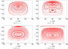 |
Fig. 1 Poincaré sections shown in the (ω1; e1) space for mass ratio at αm = 1.1. Gray points stand for Poincaré sections produced under the quadrupole-order model and red points stand for the ones produced under the octupole-order Hamiltonian model. The section is defined by g2 = π/2. The island centers and their corresponding Hamiltonians are marked in the left panel of Fig. 3. In panel (b), the centers of libration islands arising in the Poincaré section under the octupole-order model are marked by black stars and they are as examples to analyze the arguments of secondary resonance, as shown in Fig. 7. |
3.2 Periodic orbits
It is known that there is a correspondence between (stable) periodic orbits and the libration island in the Poincaré section. Therefore, we illustrate the bifurcation phenomenon from the viewpoint of periodic orbits associated with ZLK resonance.
In the Hamiltonian model truncated at the quadrupole order (which is an integrable model), if the initial condition (g1,0, G1,0) is at the exact resonance center of the ZLK resonance, g1 and G1 will remain stationary (Lei & Huang 2022). However, when the octupole-order terms are included, the resulting Hamiltonian determines a 2-DOF model. Starting from the ZLK resonance center, g1 and G1 may evolve over time and finally constitute a closed curve in the (g1, G1) space, representing a periodic orbit. In particular, an exact periodic orbit associated with the ZLK resonance should have minimum oscillation. Furthermore, when the (e.g., Hamiltonian) parameter is changed, periodic orbits may constitute a certain family, which can be uniquely characterized by their initial values (Deprit & Henrard 1967). The trace of resonance center in a certain parameter space is referred to as the characteristic curves of periodic orbit families.
We can see that the curves of the ZLK resonance center under the quadrupole-order Hamiltonian model are replaced by the characteristic curves of periodic orbit families associated with ZLK resonance under the octupole-order Hamiltonian model. Therefore, it becomes possible for us to study dynamics associated with ZLK resonances by computing periodic orbits under the octupole-level approximation.
Regarding the determination of periodic orbits families, there are numerous available methods. The predictor-corrector algorithm is widely used for solving two-point boundary-value problems (Deprit & Henrard 1967). For convenience, this work starts from the Poincaré section, based on the consideration that the (stable) periodic orbits correspond to the libration island centers arising in the Poincaré section. For a certain periodic orbit associated with ZLK resonance, the oscillation amplitude of the argument g1 should reach its minimum, meaning that finding a periodic orbit is equivalent to solving an optimisation problem. In practice, we utilized the spline interpolation method combined with a local minima search algorithm to determine the location of periodic orbit, corresponding to libration centers of ZLK resonance under the octupole-order Hamiltonian model. We suggest the reader to refer to Huang & Lei (2024) for a different algorithms for producing periodic orbit families.
Figure 3 shows the curves of the conventional ZLK center under the quadrupole order and characteristic curves of periodic orbit families associated with ZLK resonance under the octupole-order Hamiltonian model. In particular, three cases with mass ratios at αm = 1.1, 25, 40 are taken into account, and the bifurcation phenomenon can be observed in these three cases. It also shows that the phenomenon of bifurcation commonly existed in a wide range of mass ratios.
In the case of αm = 1.1, there are two bifurcation points, and, in the cases of αm = 25,40, there is a single bifurcation point across the families, showing that the dynamical structures may be more complex for the cases with lower mass ratios. With an increase in mass ratio, αm, the bifurcation happens at a higher eccentricity. It means that it is more difficult to trigger the phenomenon of bifurcation at a higher mass ratio, αm. In particular, when αm → ∞, corresponding to the so-called restricted hierarchical three-body problem, it is predicted that the bifurcation happens at eccentricity-approach unity. This is why we cannot observe bifurcations under the test-particle approximations where αm → ∞ in previous studies (Lei 2022; Lei & Gong 2022).
In addition, we can see that the characteristic curves of periodic orbit families and the curves of the ZLK resonance center are in good agreement in the region far away from the bifurcation points, while they show a larger deviation in the region closer to the bifurcation points. In the left and right panels of Fig. 3, some representative points near the bifurcation points are marked by hollow circles, and their associated Poincaré sections are presented in Figs. 1 and 2. There is a good correspondence between the distribution of periodic orbits and dynamical structures arising in Poincaré sections. In particular, a single periodic orbit indicates that there is a single island of libration, and two periodic orbits show that there are two libration islands in the Poincaré section. It is not difficult to understand such a correspondence, because the center of the islands usually corresponds a stable periodic orbit under a 2-DOF dynamical model. The characteristic curves shown in panels a and c of Fig. 3 can help us to understand the different behaviors observed in Poincaré sections for the cases of αm = 1.1 and αm = 40.
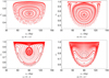 |
Fig. 2 Similar to Fig. 1, but for the mass ratio at αm = 40. The island centers and their corresponding Hamiltonian are marked in the right panel of Fig. 3. |
3.3 Influence on excitation of eccentricity
According to discussions on Poincaré sections and periodic orbit families associated with ZLK resonance, we can see that the phenomenon of bifurcation can exist under the dynamical model in a large range of mass ratios, but under a certain Hamiltonian interval [ℋc,1, ℋc,2] where the boundaries ℋc,1 and ℋc,2 are dependent on mass ratio.
In order to illustrate the influence of bifurcation upon eccentricity excitation during the long-term evolution, we take two representative cases as examples, under the given Hamiltonian at ℋ = 1.8. One of them, with an initial eccentricity at e1,0 = 0.436, is close to the bifurcation; and the other one, with an initial eccentricity at e1,0 = 0.2, is far away from it. Their trajectories are numerically propagated under both the quadrupole- and octupole-order Hamiltonian models, and the associated oscillations of eccentricity and mutual inclination are shown in Fig. 4, where the trajectories under the quadrupole-order model are shown by blue lines, and the ones under the octupole-order model are shown by red dots (see the caption for detailed settings of initial conditions). For comparison, the characteristic curves of periodic orbit families and curves of the ZLK resonance center are presented as the background.
From Fig. 4, one can see that (a) the trajectories under the quadruple-order model are periodic and smooth because of the presence of a motion integral G2(Gtot, e1, itot); (b) the trajectories propagated under the octupole-order model are no longer periodic, and a certain spread in the (itot, e1) space can be observed; (c) for the case close to the bifurcation point (see the left panel), the trajectory under the quadrupole-order model (corresponding to the conventional ZLK resonance) has small eccentricity excitation, but it has a much larger excitation of eccentricity for the trajectory under the octupole-order model; and (d) for the case far away from the bifurcation point (see the right panel), it is observed that there are comparable eccentricity excitations for trajectories under the quadrupole- and octupole-order models. According to such a comparative analysis, we can conclude that the phenomenon of bifurcation can enhance the excitation of planetary eccentricity and/or inclination during the long-term evolution in comparison with the conventional ZLK resonance, especially in the region near the bifurcation points.
To clearly illustrate the influence of the bifurcation phenomenon, it is meaningful to analyze dynamical systems with different Hamiltonians by considering different mass ratios. The methodology is to numerically integrate the equations of motion under the quadrupole- and octupole-order Hamiltonian models, and compute the maximum eccentricity reached over a long enough period. Results are shown in Fig. 5, where the maximum eccentricities are given as functions of Hamiltonian ℋ. In particular, two cases of mass ratios at αm = 1.1 (standing for the case of low mass ratio) and αm = 40 (standing for the case of high mass ratio) are considered.
From Fig. 5, it is observed that (a) in the region far away from the bifurcation point, the maximum eccentricities under the quadrupole- and octupole-order models are qualitatively comparable; (b) in the region near the bifurcation point, the maximum eccentricity under the octupole-order model is higher than that of the quadrupole-order model; (c) the effect of enhancement is stronger when the initial state is closer to the bifurcation point; and (d) the effect of enhancement is stronger when the dynamical model has a lower mass ratio αm (it is weaker for a higher mass ratio). Point (d) is not difficult to understand because, when the mass ratio αm is high, the bifurcation phenomenon happens at an eccentricity closer to unity, limiting the excitation eccentricity.
In summary, bifurcations of the periodic orbit family associated with ZLK resonance under the octupole order significantly influence the eccentricity excitation when compared to the conventional ZLK effect. The bifurcation phenomenon exists in a vast mass-ratio range, and its emergence is limited to a certain Hamiltonian range: [ℋc,1, ℋc,2]. Therefore, if an actual planetary system is situated within this region, considering the octupole-order term is imperative when studying the long-term dynamics inside ZLK resonance. In the coming section, we intend to perform a perturbation analysis in order to shed light on this phenomenon and clarify the dynamical mechanism that is responsible for the phenomenon of bifurcation.
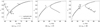 |
Fig. 3 Distribution of ZLK center determined under the quadrupole-order model (dashed lines) and characteristic curves of periodic orbits determined under the octupole-order model (solid lines) in the (itot, e1) space for mass ratios at αm=1.1,25,40. To determine periodic orbits associated with ZLK resonance, the initial angles are fixed at g1,0 = g2,0 = π/2. The points marked by hollow circles in panels a and c are taken as examples to produce Poincaré sections, as shown in Figs. 1 and 2. |
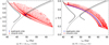 |
Fig. 4 Oscillations of eccentricity and mutual inclination for numerically propagated trajectories corresponding to ℋ = 1.8 with mass ratio at αm = 1.1 for different initial eccentricities at e1,0 = 0.436 (left panel) and e1,0 = 0.2 (right panel). Both the initial conditions of g1 and g2 are assumed at π/2. Red points represent the trajectories numerically propagated under the octupole-order Hamiltonian, while the blue lines stand for the trajectories numerically propagated under the quadrupole-order model. For comparison, the characteristic curves of periodic orbit families associated with ZLK resonance and the conventional ZLK resonance centers are provided (see the solid black lines and the dashed lines, which are the same as the ones shown in Fig. 3). |
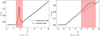 |
Fig. 5 Maximum eccentricity reached by the trajectories is shown as a function of the Hamiltonian ℋ for the cases of αm = 1.1 (left panel) and αm = 40 (right panel). The solid lines represent the curves determined under the octupole-order model, while the dashed lines represent the curves determined under the quadrupole-order model. The initial eccentricities are assumed at 0.45 for αm = 1.1 and 0.6 for αm = 40. Under the octupole-order model, the peak of e1,max happens near the bifurcation point. It is observed that, in the region near the bifurcation point (see the shaded region), the maximum eccentricities reached under the quadrupole- and octupole-order Hamiltonian models have significant differences, while in the region far away from the bifurcation point they have no differences. This means that the octupole-order terms contribute significantly to the excitation of eccentricity in those regions near the bifurcation point. |
4 Analytical study
In this section, we study the dynamics inside ZLK resonance under the octupole-order Hamiltonian through perturbative treatments. The octupole-order Hamiltonian function is written as follows:
![Mathematical equation: $\[\mathcal{H}=\mathcal{H}_2\left(g_1, G_1, G_2\right)+\mathcal{H}_3\left(g_1, g_2, G_1, G_2\right) .\]$](/articles/aa/full_html/2024/09/aa50912-24/aa50912-24-eq12.png)
Usually, the octupole-order term ℋ3 is much smaller than the quadrupole-order term ℋ2 in terms of magnitude. Therefore, from the viewpoint of perturbation theory, we can take the octupole-order term ℋ3 as the perturbation to the quadrupole-order dynamics.
4.1 Introduction of action-angle variables
The unperturbed dynamical model determined by the quadrupole-order Hamiltonian ℋ2 is an integrable system, where G2 is an integral of motion. Thus, it is possible to introduce a set of action-angle variables under the unperturbed Hamiltonian model as follows (Morbidelli 2002; Lei & Huang 2022):
![Mathematical equation: $\[\begin{aligned}& g_1^*=g_1-\rho_1=\frac{2 \pi}{T_1} t, \quad G_1^*=\frac{1}{2 \pi} \oint G_1 \mathrm{~d} g_1, \\& g_2^*=g_2-\rho_2=g_{2,0}+\frac{2 \pi}{T_2} t, \quad G_2^*=G_2,\end{aligned}\]$](/articles/aa/full_html/2024/09/aa50912-24/aa50912-24-eq13.png) (5)
(5)
where T1 and T2 are periods of g1 and g2, respectively. ρ1 and ρ2 are periodic functions of time with zero average, and they hold the same period T1 of g1 along the closed ZLK cycle. ![Mathematical equation: $\[G_1^*\]$](/articles/aa/full_html/2024/09/aa50912-24/aa50912-24-eq14.png) represents the path integration of the ZLK cycle in the (g1, G1) space (divided by 2π), and it is the so-called Arnold action. g2,0 is the angle of g2 at the initial instant. It is evident that the angles after transformation
represents the path integration of the ZLK cycle in the (g1, G1) space (divided by 2π), and it is the so-called Arnold action. g2,0 is the angle of g2 at the initial instant. It is evident that the angles after transformation ![Mathematical equation: $\[g_1^*\]$](/articles/aa/full_html/2024/09/aa50912-24/aa50912-24-eq15.png) and
and ![Mathematical equation: $\[g_2^*\]$](/articles/aa/full_html/2024/09/aa50912-24/aa50912-24-eq16.png) becomes linear functions of time t.
becomes linear functions of time t.
In terms of the set of action-angle variables, the quadrupole-order Hamiltonian becomes
![Mathematical equation: $\[\mathcal{H}_2\left(g_1, g_2, G_1\right) \Rightarrow \mathcal{H}_2\left(G_1^*, G_2^*\right),\]$](/articles/aa/full_html/2024/09/aa50912-24/aa50912-24-eq17.png) (6)
(6)
which is of normal form. Under the unperturbed Hamiltonian model, the fundamental frequencies are determined by
![Mathematical equation: $\[\dot{g}_1^*=\frac{2 \pi}{T_1}=\frac{\partial \mathcal{H}_2\left(G_1^*, G_2^*\right)}{\partial G_1^*}, \quad \dot{g}_2^*=\frac{2 \pi}{T_2}=\frac{\partial \mathcal{H}_2\left(G_1^*, G_2^*\right)}{\partial G_2^*}.\]$](/articles/aa/full_html/2024/09/aa50912-24/aa50912-24-eq18.png) (7)
(7)
If there is a commensurability between the fundamental frequencies, secular resonances happen between ![Mathematical equation: $\[g_1^*\]$](/articles/aa/full_html/2024/09/aa50912-24/aa50912-24-eq19.png) and
and ![Mathematical equation: $\[g_2^*\]$](/articles/aa/full_html/2024/09/aa50912-24/aa50912-24-eq20.png) , and the resonant condition is given by
, and the resonant condition is given by
![Mathematical equation: $\[k_1 \dot{g}_1^*-k_2 \dot{g}_2^*=0.\]$](/articles/aa/full_html/2024/09/aa50912-24/aa50912-24-eq21.png) (8)
(8)
where k1 ∈ ℕ and k2 ∈ ℤ. As we focus on the motions inside ZLK resonance, secular resonances satisfying Equation (8) are referred to as ZLK secondary k2:k1 resonances.
By solving Equation (8), it is possible to obtain the nominal position of secondary resonances between ![Mathematical equation: $\[g_1^*\]$](/articles/aa/full_html/2024/09/aa50912-24/aa50912-24-eq23.png) and
and ![Mathematical equation: $\[g_2^*\]$](/articles/aa/full_html/2024/09/aa50912-24/aa50912-24-eq24.png) . Fig. 6 shows the nominal location of the ZLK secondary resonances via dashed red lines in the (itot, e1) space. The left panel is for the case of αm = 1.1, and the right panel is for the case of αm = 40. For ease of comparison, the curves of conventional the ZLK resonance center (dashed black lines), characteristic curves of periodic orbit families associated with ZLK resonance (solid black lines), and level curves of octupole-order Hamiltonian (gray lines) are provided as a background. It is observed that bifurcations of periodic orbit families associated with ZLK resonance correspond well to ZLK secondary resonances. In particular, in the case of a low mass ratio (αm = 1.1), there are two bifurcation points, which correspond to ZLK secondary 2:1 and 3:1 resonances (see the left panel, where the influence of secondary 3:1 resonance is weak) and, in the case of a high mass ratio (αm = 40), the bifurcation of periodic orbit family corresponds to ZLK secondary 2:1 resonance (see the right panel where the secondary 3:1 resonance disappears). Motivated by such a good correspondence, we may ask if the phenomenon of bifurcation triggered by ZLK secondary resonance.
. Fig. 6 shows the nominal location of the ZLK secondary resonances via dashed red lines in the (itot, e1) space. The left panel is for the case of αm = 1.1, and the right panel is for the case of αm = 40. For ease of comparison, the curves of conventional the ZLK resonance center (dashed black lines), characteristic curves of periodic orbit families associated with ZLK resonance (solid black lines), and level curves of octupole-order Hamiltonian (gray lines) are provided as a background. It is observed that bifurcations of periodic orbit families associated with ZLK resonance correspond well to ZLK secondary resonances. In particular, in the case of a low mass ratio (αm = 1.1), there are two bifurcation points, which correspond to ZLK secondary 2:1 and 3:1 resonances (see the left panel, where the influence of secondary 3:1 resonance is weak) and, in the case of a high mass ratio (αm = 40), the bifurcation of periodic orbit family corresponds to ZLK secondary 2:1 resonance (see the right panel where the secondary 3:1 resonance disappears). Motivated by such a good correspondence, we may ask if the phenomenon of bifurcation triggered by ZLK secondary resonance.
To illustrate this problem, two periodic trajectories, located at island centers, as shown in panel (b) of Fig. 1, are taken as examples. Their time histories of the arguments associated with ZLK secondary 2:1 resonance are shown in Fig. 7. It is observed that the argument is librating around zero (or π) for the trajectory shown in the left (or right) panel and the oscillation amplitude is small. Indeed, both periodic orbits are inside ZLK secondary 2:1 resonance. Additional simulations show that quasi-periodic orbits arising in Poincaré sections are also inside secondary 2:1 resonance.
Based on the above discussions, we can come to the conclusion that bifurcations of periodic orbit families associated with ZLK resonance are induced by ZLK secondary resonances. In this sense, we could study the dynamics of ZLK secondary resonances, which may help us to understand the phenomenon of bifurcation.
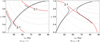 |
Fig. 6 Nominal location of ZLK secondary 2:1 and 3:1 resonances (see red dashed lines), determined by fundamental frequencies for different mass ratios at αm = 1.1 (left panel) and αm = 40 (right panel). For comparison, the characteristic curves of periodic families associated with ZLK resonance (solid blue lines), the conventional ZLK resonant centers (black stars), and the level curves of octupole-order Hamiltonian (gradient gray curves) are presented as background. It is observed that there is a good correspondence between the nominal location of ZLK secondary resonances and the bifurcation points of periodic orbit families. |
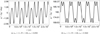 |
Fig. 7 Time histories of the arguments |
![Mathematical equation: $\[g_1^*{-}2 g_2^*\]$](/articles/aa/full_html/2024/09/aa50912-24/aa50912-24-eq22.png)
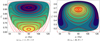 |
Fig. 8 Phase portraits (level curves of adiabatic invariant J with given Hamiltonian ℋ) for the cases of αm = 1.1 (ℋ = 1.9), αm = 40 (ℋ = 7) in the (g1, G1) space. For convenience of comparison, the associated Poincaré sections are presented as background (see the red dots). |
4.2 Perturbative treatments
In terms of action-angle variables, the octupole-level Hamiltonian function can be expressed as follows:
![Mathematical equation: $\[\mathcal{H}=\mathcal{H}_2\left(G_1^*, G_2^*\right)+\mathcal{H}_3\left(g_1^*, g_2^*, G_1^*, G_2^*\right),\]$](/articles/aa/full_html/2024/09/aa50912-24/aa50912-24-eq25.png) (9)
(9)
where ℋ2 is the kernel function and ℋ3 can be regarded as the perturbation term. In order to study ZLK secondary resonances, we need to introduce an additional canonical transformation,
![Mathematical equation: $\[\begin{aligned}& \sigma_1=g_1^*-\frac{k_2}{k_1} g_2^*, \quad \Sigma_1=G_1^*, \\&\qquad\qquad\qquad\qquad\qquad\qquad\quad,\\& \sigma_2=g_2^*, \quad \Sigma_2=\frac{k_2}{k_1} G_1^*+G_2^*.\end{aligned}\]$](/articles/aa/full_html/2024/09/aa50912-24/aa50912-24-eq26.png) (10)
(10)
where σ1 is the argument of secondary k2:k1 resonance. Up to now, we formulated the following mutual transformations among different sets of canonical variables:
![Mathematical equation: $\[\left(g_1, G_1, g_2, G_2\right) \Longleftrightarrow\left(g_1^*, G_1^*, g_2^*, G_2^*\right) \Longleftrightarrow\left(\sigma_1, \Sigma_1, \sigma_2, \Sigma_2\right) .\]$](/articles/aa/full_html/2024/09/aa50912-24/aa50912-24-eq27.png)
In terms of the final set of canonical variables, the octupole-order Hamiltonian can be further organized as
![Mathematical equation: $\[\mathcal{H}=\mathcal{H}_2\left(\Sigma_1, \Sigma_2\right)+\mathcal{H}_3\left(\sigma_1, \sigma_2, \Sigma_1, \Sigma_2\right).\]$](/articles/aa/full_html/2024/09/aa50912-24/aa50912-24-eq28.png) (11)
(11)
In particular, when the planetary system is inside a certain ZLK secondary k2:k1 resonance, it holds ![Mathematical equation: $\[\dot{\sigma}_1 \approx 0\]$](/articles/aa/full_html/2024/09/aa50912-24/aa50912-24-eq29.png) . Thus, the frequencies satisfy the hierarchical relation
. Thus, the frequencies satisfy the hierarchical relation ![Mathematical equation: $\[\dot{\sigma}_1 \ll \dot{\sigma}_2\]$](/articles/aa/full_html/2024/09/aa50912-24/aa50912-24-eq30.png) , meaning that the argument σ1 is a long-period variable (i.e., slow variable), while σ2 is a short-period variable (i.e., fast variable). In other words, Equation (11) determines a typical separable Hamiltonian model (Henrard 1990).
, meaning that the argument σ1 is a long-period variable (i.e., slow variable), while σ2 is a short-period variable (i.e., fast variable). In other words, Equation (11) determines a typical separable Hamiltonian model (Henrard 1990).
Under the separable Hamiltonian model, the pair of variables (σ1, Σ1) stands for the slow degree of freedom, and the other one (σ2, Σ2) stands for the fast degree of freedom. According to Wisdom (1985), the variables associated with the slow degree of freedom can be assumed as parameters when we are exploring the dynamics during the timescale of the fast degree of freedom. Under this approximation, the resulting Hamiltonian determines an integrable dynamical model with (σ2, Σ2) as phase-space variables, and the following action-angle variables can be introduced (Morbidelli 2002):
![Mathematical equation: $\[\phi=\frac{2 \pi}{T} t, \quad J=\frac{1}{2 \pi} \int_0^{2 \pi} \Sigma_2 \mathrm{d} \sigma_2,\]$](/articles/aa/full_html/2024/09/aa50912-24/aa50912-24-eq31.png) (12)
(12)
where J stands for the path integration of the integrable Hamiltonian model in the (σ2, Σ2) space (divided by 2π). By taking advantage of the set of canonical variables (ϕ, J), the octupoleorder Hamiltonian can be further expressed as
![Mathematical equation: $\[\mathcal{H}=\mathcal{H}_2\left(\Sigma_1, J\right)+\mathcal{H}_3\left(\sigma_1, \Sigma_1, J\right),\]$](/articles/aa/full_html/2024/09/aa50912-24/aa50912-24-eq32.png) (13)
(13)
where the angle ϕ becomes a cyclic variable, showing that the action variable J is a motion integral in the long-term evolution. Usually, the motion integral J is called adiabatic invariant. Evidently, there are two conserved quantities including the Hamiltonian ℋ and the adiabatic invariant J for the current 2-DOF Hamiltonian model. Therefore, the current Hamiltonian model becomes approximately integrable.
4.3 Phase-space structures of ZLK secondary resonances
As discussed above, when a planetary system is located inside a certain ZLK secondary resonance, the resulting Hamiltonian can be approximated as an integrable model by introducing an adiabatic invariant. For such an integrable Hamiltonian model, its phase-space structures can be explored by analyzing phase portraits. There are two approaches to generating phase portraits (Lei & Gong 2022): (a) plotting level curves of the Hamiltonian ℋ with a given adiabatic invariant, J; and (b) plotting level curves of a adiabatic invariant, J, with a given Hamiltonian, ℋ. Without a doubt, two versions of phase portraits are equivalent. In this work, the latter version was adopted.
As for the ZLK secondary 2:1 resonance, Fig. 8 presents phase portraits in the (g1, G1) space for the cases of mass ratios at αm = 1.1,40. For convenience of comparison, their associated Poincaré sections at the same Hamiltonian are provided as a background (see the red dots). We can see that dynamical structures are different between the cases of αm=1.1 and the case of αm=40. In particular, there is an excellent agreement between analytical structures arising in phase portraits and numerical structures arising in Poincaré sections, meaning that numerical structures associated with bifurcations can be analytically reproduced. Therefore, we can conclude that the phenomenon of bifurcation arising in Poincaré sections is indeed triggered by ZLK secondary resonance.
By analysing phase portraits associated with ZLK secondary 2:1 resonance, it is possible for us to determine the location of the resonant center. For the cases of mass ratios at αm=l.l,40, the distribution of resonant center is shown in Fig. 9 (see solid red circles). For ease of comparison, the characteristic curves of periodic orbit families (see solid black lines), the conventional ZLK center curves (see dashed black lines) and level curves of octupole-order Hamiltonian (see gray lines) are provided as a background. We can see that ZLK secondary resonance exists in a small range of Hamiltonian levels [ℋc,1, ℋc,2]. In the region near the bifurcation point, the libration center of ZLK secondary resonance can agree well with the characteristic curves of periodic orbit families under the octupole-order Hamiltonian model. Due to the emergence of ZLK secondary resonance, dynamical structures becomes more complex than the conventional phase portraits of the primary ZLK resonance.
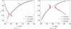 |
Fig. 9 Libration centers of ZLK secondary 2:1 resonances determined by analyzing phase portraits (solid red circles) for different mass ratios at αm = 1.1 (left panel) and αm = 40 (right panel). For comparison, the characteristic curves of periodic families associated with ZLK resonance, the conventional ZLK centers and level curves of octupole-order Hamiltonian are presented (see the solid blue, red dashed, and gray lines). There is a good correspondence between the center of ZLK secondary resonance and the characteristic curves of periodic orbit families in the region near the bifurcation point. |
5 Applications to exoplanetary systems
In this section, three actual exoplanet systems (including HAT-P-11, HAT-P-13, and HAT-P-44) are chosen for practical applications (see Table 1 for their parameters). Mass ratios of these three systems are αm > 10, corresponding to a high-mass-ratio case. We expect their dynamical structures to be similar to the right panel of Fig. 8.
Considering the fact that the inclination data are absent for the latter two systems, we assume their mutual inclination between the inner and outer planetary orbits as itot = 45° for practical simulations. Under this assumption, the total angular momentum is, respectively, equal to 150.67, 66.62, and 58.83 for these three systems.
Results are given in Fig. 10, where the left column’s panels present phase portraits of ZLK secondary 2:1 resonance and the associated Poincaré sections, and the right column’s panels show the distribution of the center of secondary 2:1 resonance by analyzing phase portraits (curves of conventional ZLK resonance are provided as background). As desired, these three exoplanetary systems hold qualitatively similar structures. In particular, bifurcation may happen for them, leading to complex dynamical structures in phase space. Comparisons made in the left column’s panels show that numerical structures arising in Poincaré sections can be well reproduced using an analytical approach. It means that the bifurcation phenomenon is triggered by ZLK secondary 2:1 resonance. The right column’s panels show that the ZLK secondary 2:1 resonance exists in a certain Hamiltonian range: [ℋc,1, ℋc,2].
When the Hamiltonian of an exoplanetary system is located in the range, [ℋc,1, ℋc,2], corresponding to the bifurcation, the ZLK secondary 2:1 resonance may occur, and it is inclined to excite a larger eccentricity of the exoplanet orbit. This mechanism may amplify the impact of the ZLK effect on the evolutionary trajectory of the exoplanet, such as a hot Jupiter.
Orbital parameters of exoplanet systems (NASA Exoplanet Archive 2024).
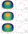 |
Fig. 10 Phase portraits and Poincaré sections (left column panels) and ZLK secondary resonant centers (right-column panels) for exoplanetary systems HAT-P-11, HAT-P-13, and HAT-P-44 systems (from top to bottom). For comparison, the ZLK centers under the quadrupole order and level curves of octupole-order Hamiltonians are presented as background (see the black dashed and gray lines, respectively). |
6 Conclusion
In this work, an intriguing phenomenon of bifurcation arising in Poicnaré sections and characteristic curves of periodic orbit families associated with ZLK resonance is systematically investigated under the double-averaged Hamiltonian model formulated up to the octupole order in the semimajor axis ratio α = a1/a2.
Practical simulations show that the phenomenon of bifurcation inside the ZLK resonance exists in planetary systems with a large range of mass ratios. The bifurcation point moves to a higher-eccentricity space with the increase of mass ratio. In particular, when the mass ratio approaches infinity (corresponding to the inner test-particle case), bifurcation is expected to happen at an eccentricity close to unity, which may help us to understand the reason why the phenomenon of bifurcation is not found in previous literature under the restricted hierarchical planetary configurations. In the region near the bifurcation point, dynamical structures inside the ZLK resonance are distinctively different between the quadrupole- and octupole-order Hamiltonian models due to the emergence of bifurcation. However, in the region far away from the bifurcation point, there is no qualitative difference between them. There is a good correspondence between the characteristic curves of periodic orbit families associated with ZLK resonance and dynamical structures of Poincaré sections, which is due to the fact that the stable periodic orbit is usually located at the center of the libration island in a Poincaré section. The phenomenon of bifurcation could lead to stronger excitation of planetary eccentricity and/or inclination, and the level of enhancement is dependent on the initial eccentricity.
By analyzing fundamental frequencies, we find that there is a good correspondence between the location of bifurcation point and the nominal location of ZLK secondary resonance. By introducing a series of canonical transformations, we come to the conclusion that the bifurcation phenomenon is triggered by ZLK secondary resonances.
When a planetary system is located inside a certain ZLK secondary resonance, the octupole-order Hamiltonian determines a separable dynamical model, which can be further approximated as an integrable system by introducing an adiabatic invariant. Dynamical structures associated with ZLK secondary resonance can be explored by analyzing phase portraits (level curves of adiabatic invariant with a given Hamiltonian). There is a perfect agreement between the analytical structures arising in phase portraits and numerical structures arising in Poincaré sections, showing that the phenomenon of bifurcation is indeed induced by ZLK secondary resonance.
The analytical approach is applied to three exoplanetary systems: HAT-P-11, HAT-P-13, and HAT-P-44. Results show that these three systems exhibit ZLK secondary 2:1 resonance within a certain Hamiltonian range. Inside ZLK secondary resonance, larger planetary eccentricity and/or inclination excitation is expected.
Acknowledgements
This work is supported by the National Natural Science Foundation of China (Nos. 12073011 and 12233003) and the National Key R&D Program of China (No. 2019YFA0706601).
References
- Bailey, M. E., Chambers, J. E., & Hahn, G. 1992, A&A, 257, 315 [NASA ADS] [Google Scholar]
- Beust, H., Bonfils, X., Montagnier, G., Delfosse, X., & Forveille, T. 2012, A&A, 545, A88 [NASA ADS] [CrossRef] [EDP Sciences] [Google Scholar]
- Blaes, O., Lee, M., & Socrates, A. 2002, ApJ, 578, 775 [NASA ADS] [CrossRef] [Google Scholar]
- Cheetham, A., Ségransan, D., Peretti, S., et al. 2017, A&A, 614, A16 [Google Scholar]
- Dawson, R. I., & Johnson, J. A. 2018, ARA&A, 56, 175 [Google Scholar]
- Deprit, A., & Henrard, J. 1967, AJ, 72, 158 [NASA ADS] [CrossRef] [Google Scholar]
- Fabrycky, D., & Tremaine, S. 2007, ApJ, 669, 1298 [NASA ADS] [CrossRef] [Google Scholar]
- Ford, E. B., Kozinsky, B., & Rasio, F. A. 2000, ApJ, 535, 385 [NASA ADS] [CrossRef] [Google Scholar]
- Fragione, G., & Antonini, F. 2019, MNRAS, 488, 728 [CrossRef] [Google Scholar]
- Hansen, B., & Naoz, S. 2020, MNRAS, 499, 1682 [NASA ADS] [CrossRef] [Google Scholar]
- Harrington, R. S. 1968, AJ, 73, 190 [NASA ADS] [CrossRef] [Google Scholar]
- Harrington, R. S. 1969, Celest. Mech., 1, 200 [NASA ADS] [CrossRef] [Google Scholar]
- Henrard, J. 1990, Celest. Mech. Dyn. Astron., 49, 43 [NASA ADS] [CrossRef] [Google Scholar]
- Huang, X., & Lei, H. 2022, AJ, 164, 232 [NASA ADS] [CrossRef] [Google Scholar]
- Huang, X., & Lei, H. 2024, AJ, 167, 234 [NASA ADS] [CrossRef] [Google Scholar]
- Ito, T., & Ohtsuka, K. 2019, Monogr. Environ. Earth Planets, 7, 1 [Google Scholar]
- Kozai, Y. 1962, AJ, 67, 591 [Google Scholar]
- Krymolowski, Y., & Mazeh, T. 1999, MNRAS, 304, 720 [NASA ADS] [CrossRef] [Google Scholar]
- Lei, H. 2020, Astrodynamics, 4, 57 [NASA ADS] [CrossRef] [Google Scholar]
- Lei, H. 2022, AJ, 163, 214 [NASA ADS] [CrossRef] [Google Scholar]
- Lei, H., & Gong, Y. 2022, A&A, 665, A62 [NASA ADS] [CrossRef] [EDP Sciences] [Google Scholar]
- Lei, H., & Huang, X. 2022, MNRAS, 515, 1086 [NASA ADS] [CrossRef] [Google Scholar]
- Lei, H., Ortore, E., & Circi, C. 2022, Astrodynamics, 6, 357 [CrossRef] [Google Scholar]
- Li, G., Naoz, S., Holman, M., & Loeb, A. 2014a, ApJ, 791, 86 [NASA ADS] [CrossRef] [Google Scholar]
- Li, G., Naoz, S., Kocsis, B., & Loeb, A. 2014b, ApJ, 785, 116 [NASA ADS] [CrossRef] [Google Scholar]
- Lidov, M. 1962, Planet. Space Sci., 9, 719 [Google Scholar]
- Lithwick, Y., & Naoz, S. 2011, ApJ, 742, 94 [NASA ADS] [CrossRef] [Google Scholar]
- Martin, R. G., Nixon, C., Lubow, S. H., et al. 2014, ApJ, 792, L33 [Google Scholar]
- Michel, P., & Thomas, F. 1996, A&A, 307, 310 [NASA ADS] [Google Scholar]
- Morbidelli, A. 2002, Modern Celestial Mechanics: Aspects of Solar System Dynamics (London and New York: Taylor & Francis) [Google Scholar]
- Naoz, S. 2016, ARA&A, 54, 441 [Google Scholar]
- Naoz, S., Perets, H. B., & Ragozzine, D. 2010, ApJ, 719, 1775 [NASA ADS] [CrossRef] [Google Scholar]
- Naoz, S., Farr, W. M., Lithwick, Y., Rasio, F. A., & Teyssandier, J. 2011, Nature, 473, 187 [NASA ADS] [CrossRef] [Google Scholar]
- Naoz, S., Farr, W. M., & Rasio, F. A. 2012, ApJ, 754, L36 [NASA ADS] [CrossRef] [Google Scholar]
- Naoz, S., Farr, W. M., Lithwick, Y., Rasio, F. A., & Teyssandier, J. 2013, MNRAS, 431, 2155 [NASA ADS] [CrossRef] [Google Scholar]
- NASA Exoplanet Archive 2024, Planetary Systems (USA: NASA) [Google Scholar]
- Petrovich, C. 2015, ApJ, 805, 75 [NASA ADS] [CrossRef] [Google Scholar]
- Safarzadeh, M., Hamers, A. S., Loeb, A., & Berger, E. 2020, ApJ, 888, L33 [NASA ADS] [CrossRef] [Google Scholar]
- Sidorenko, V. V. 2018, Celest. Mech. Dyn. Astron., 130, 67 [CrossRef] [Google Scholar]
- Subr, L., & Karas, V. 2005, A&A, 433, 405 [NASA ADS] [CrossRef] [EDP Sciences] [Google Scholar]
- Takeda, G., & Rasio, F. A. 2005, ApJ, 627, 1001 [Google Scholar]
- Tamuz, O., Ségransan, D., Udry, S., et al. 2008, A&A, 480, L33 [NASA ADS] [CrossRef] [EDP Sciences] [Google Scholar]
- Teyssandier, J., Naoz, S., Lizarraga, I., & A. Rasio, F. 2013, ApJ, 779, 166 [NASA ADS] [CrossRef] [Google Scholar]
- Thompson, T. A. 2011, ApJ, 741, 82 [NASA ADS] [CrossRef] [Google Scholar]
- von Zeipel, H. 1910, Astron. Nachr., 183, 345 [Google Scholar]
- Wegg, C., & Bode, J. N. 2011, ApJ, 738, L8 [NASA ADS] [CrossRef] [Google Scholar]
- Wisdom, J. 1985, Icarus, 63, 272 [Google Scholar]
- Zhao, G., Xie, J., Zhou, J., & Lin, D. 2012, ApJ, 749, 172 [NASA ADS] [CrossRef] [Google Scholar]
All Tables
All Figures
|
Fig. 1 Poincaré sections shown in the (ω1; e1) space for mass ratio at αm = 1.1. Gray points stand for Poincaré sections produced under the quadrupole-order model and red points stand for the ones produced under the octupole-order Hamiltonian model. The section is defined by g2 = π/2. The island centers and their corresponding Hamiltonians are marked in the left panel of Fig. 3. In panel (b), the centers of libration islands arising in the Poincaré section under the octupole-order model are marked by black stars and they are as examples to analyze the arguments of secondary resonance, as shown in Fig. 7. |
| In the text | |
|
Fig. 2 Similar to Fig. 1, but for the mass ratio at αm = 40. The island centers and their corresponding Hamiltonian are marked in the right panel of Fig. 3. |
| In the text | |
|
Fig. 3 Distribution of ZLK center determined under the quadrupole-order model (dashed lines) and characteristic curves of periodic orbits determined under the octupole-order model (solid lines) in the (itot, e1) space for mass ratios at αm=1.1,25,40. To determine periodic orbits associated with ZLK resonance, the initial angles are fixed at g1,0 = g2,0 = π/2. The points marked by hollow circles in panels a and c are taken as examples to produce Poincaré sections, as shown in Figs. 1 and 2. |
| In the text | |
|
Fig. 4 Oscillations of eccentricity and mutual inclination for numerically propagated trajectories corresponding to ℋ = 1.8 with mass ratio at αm = 1.1 for different initial eccentricities at e1,0 = 0.436 (left panel) and e1,0 = 0.2 (right panel). Both the initial conditions of g1 and g2 are assumed at π/2. Red points represent the trajectories numerically propagated under the octupole-order Hamiltonian, while the blue lines stand for the trajectories numerically propagated under the quadrupole-order model. For comparison, the characteristic curves of periodic orbit families associated with ZLK resonance and the conventional ZLK resonance centers are provided (see the solid black lines and the dashed lines, which are the same as the ones shown in Fig. 3). |
| In the text | |
|
Fig. 5 Maximum eccentricity reached by the trajectories is shown as a function of the Hamiltonian ℋ for the cases of αm = 1.1 (left panel) and αm = 40 (right panel). The solid lines represent the curves determined under the octupole-order model, while the dashed lines represent the curves determined under the quadrupole-order model. The initial eccentricities are assumed at 0.45 for αm = 1.1 and 0.6 for αm = 40. Under the octupole-order model, the peak of e1,max happens near the bifurcation point. It is observed that, in the region near the bifurcation point (see the shaded region), the maximum eccentricities reached under the quadrupole- and octupole-order Hamiltonian models have significant differences, while in the region far away from the bifurcation point they have no differences. This means that the octupole-order terms contribute significantly to the excitation of eccentricity in those regions near the bifurcation point. |
| In the text | |
|
Fig. 6 Nominal location of ZLK secondary 2:1 and 3:1 resonances (see red dashed lines), determined by fundamental frequencies for different mass ratios at αm = 1.1 (left panel) and αm = 40 (right panel). For comparison, the characteristic curves of periodic families associated with ZLK resonance (solid blue lines), the conventional ZLK resonant centers (black stars), and the level curves of octupole-order Hamiltonian (gradient gray curves) are presented as background. It is observed that there is a good correspondence between the nominal location of ZLK secondary resonances and the bifurcation points of periodic orbit families. |
| In the text | |
|
Fig. 7 Time histories of the arguments |
| In the text | |
|
Fig. 8 Phase portraits (level curves of adiabatic invariant J with given Hamiltonian ℋ) for the cases of αm = 1.1 (ℋ = 1.9), αm = 40 (ℋ = 7) in the (g1, G1) space. For convenience of comparison, the associated Poincaré sections are presented as background (see the red dots). |
| In the text | |
|
Fig. 9 Libration centers of ZLK secondary 2:1 resonances determined by analyzing phase portraits (solid red circles) for different mass ratios at αm = 1.1 (left panel) and αm = 40 (right panel). For comparison, the characteristic curves of periodic families associated with ZLK resonance, the conventional ZLK centers and level curves of octupole-order Hamiltonian are presented (see the solid blue, red dashed, and gray lines). There is a good correspondence between the center of ZLK secondary resonance and the characteristic curves of periodic orbit families in the region near the bifurcation point. |
| In the text | |
|
Fig. 10 Phase portraits and Poincaré sections (left column panels) and ZLK secondary resonant centers (right-column panels) for exoplanetary systems HAT-P-11, HAT-P-13, and HAT-P-44 systems (from top to bottom). For comparison, the ZLK centers under the quadrupole order and level curves of octupole-order Hamiltonians are presented as background (see the black dashed and gray lines, respectively). |
| In the text | |
Current usage metrics show cumulative count of Article Views (full-text article views including HTML views, PDF and ePub downloads, according to the available data) and Abstracts Views on Vision4Press platform.
Data correspond to usage on the plateform after 2015. The current usage metrics is available 48-96 hours after online publication and is updated daily on week days.
Initial download of the metrics may take a while.