| Issue |
A&A
Volume 627, July 2019
|
|
|---|---|---|
| Article Number | A112 | |
| Number of page(s) | 23 | |
| Section | Interstellar and circumstellar matter | |
| DOI | https://doi.org/10.1051/0004-6361/201834533 | |
| Published online | 09 July 2019 | |
Turbulent power distribution in the local interstellar medium
1
Argelander-Institut für Astronomie,
Auf dem Hügel 71,
53121 Bonn,
Germany
e-mail: This email address is being protected from spambots. You need JavaScript enabled to view it.
2
Tartu Observatory, University of Tartu,
61602 Tõravere,
Tartumaa, Estonia
Received:
29
October
2018
Accepted:
20
May
2019
Abstract
Context. The interstellar medium (ISM) on all scales is full of structures that can be used as tracers of processes that feed turbulence.
Aims. We used H I survey data to derive global properties of the angular power distribution of the local ISM.
Methods. HI4PI observations on an nside = 1024 HEALPix grid and Gaussian components representing three phases, the cold, warm, and unstable lukewarm neutral medium (CNM, WNM, and LNM), were used for velocities |vLSR|≤ 25 km s−1. For high latitudes |b| > 20° we generated apodized maps. After beam deconvolution we fitted angular power spectra.
Results. Power spectra for observed column densities are exceptionally well defined and straight in log-log presentation with 3D power law indices γ ≥−3 for the local gas. For intermediate velocity clouds (IVCs) we derive γ = −2.6 and for high velocity clouds (HVCs) γ = −2.0. Single-phase power distributions for the CNM, LNM, and WNM are highly correlated and shallow with γ ~−2.5 for multipoles l ≤ 100. Excess power from cold filamentary structures is observed at larger multipoles. The steepest single-channel power spectra for the CNM are found at velocities with large CNM and low WNM phase fractions.
Conclusions. The phase space distribution in the local ISM is configured by phase transitions and needs to be described with three distinct different phases, being highly correlated but having distributions with different properties. Phase transitions cause locally hierarchical structures in phase space. The CNM is structured on small scales and is restricted in position-velocity space. The LNM as an interface to the WNM envelops the CNM. It extends to larger scales than the CNM and covers a wider range of velocities. Correlations between the phases are self-similar in velocity.
Key words: turbulence / ISM: general / ISM: structure
© ESO 2019
1 Introduction
Turbulence is ubiquitous in the interstellar medium (ISM). Neutral hydrogen is abundant and because of the easily observable H I 21cm emission line it is one of their key diagnostics. However, there are more bearings than just diagnostics. Already in the 1950s, soon after the detection of the 21cm line, Hendrik van de Hulst had “the hope that you could do something by making a turbulence spectrum, a new trick to describe things”1. van de Hulst was interested in measuring turbulence of the H I distribution to gain insights into the nature of the ISM. Today we have a better background to formulate the question of how far turbulence is shaping the ISM and in particular the bistable H I distribution. Turbulent motions determine the temporal and spatial structure of the gas pressure. If pressure fluctuations are sufficiently large, they drive some of the gas into the cold phase. Thus, the H I phase composition is affected by turbulence. We should also expect that changes in the H I phase composition have a noticeable imprint on the observable turbulent density and velocity distribution and focused on the H I multiphase structure.
For an introduction to topics addressed in the first paragraph we refer to the reviews about interstellar turbulence by Elmegreen & Scalo (2004) and Scalo & Elmegreen (2004). Our contemporary understanding of the multiphase structure of the ISM is based on seminal papers by McKee & Ostriker (1977) and Wolfire et al. (2003). Heating and cooling processes invoke thermal instabilities that tend to segregate the H I into two distinct stable phases, the cold medium (CNM) and the warm medium (WNM). For at least two decades there has been mounting evidence that a significant fraction of the H I is in an intermediate unstable state, the lukewarm medium (LNM); for the most recent census of the phase fractions we refer to Murray et al. (2018b) and Kalberla & Haud (2018). Turbulence is considered as a driving mechanism that tends to produce strong nonlinear fluctuations in all the thermodynamic variables that are affecting thermal instabilities. Audit & Hennebelle (2005) find in this case large fractions of thermally unstable gas that would not exist without turbulent forcing. These fractions increase with the amplitude of the turbulent forcing and the cold and thermally unstable gas tends to be organized in filamentary structures. As a result, the standard two-phase model may need to be replaced by a phase continuum with at least three phases; we refer to the excellent review by Vázquez-Semadeni (2012) and references therein.
Analyzing Arecibo data, cold filamentary H I structures that are aligned with the magnetic field have been found by Clark et al. (2014) at high Galactic latitudes. Similar large-scale structures all over the sky correlated with the magnetic field orientation implied by Planck at 353 GHz polarized dust emission were reported by Kalberla et al. (2016). Some of the observed anisotropic H I structures show a clear association with magneto-ionic features (Kalberla & Kerp 2016; Kalberla et al. 2017; Jelić et al. 2018). Derived power spectra for the H I are in this case consistent with Kolmogorov turbulence, but anisotropies in narrow velocity intervals increase on average with spatial frequency, both as predicted by Goldreich & Sridhar (1995) for incompressible magnetohydrodynamic (MHD) turbulence. These observationsstrongly support an MHD origin of the turbulence similar to the conception brought forward by Heiles & Troland (2005) and Heiles & Crutcher (2005) who argued for an equipartition between turbulent and magnetic field energy.
H I observations are typically organized as data cubes in position–position-velocity (PPV). Power spectra of emission from narrow velocity channels are affected by velocity fluctuations that cause shallower slopes than spectra derived from broad channels. This is the result of an excess of small features from unrelated structures that blend by velocity crowding on the line of sight. The basic recipes used to analyze these data and disentangle velocity and density fields, called velocity channel analysis (VCA), were given by Lazarian & Pogosyan (2000). Velocity fluctuation can in principle mimic density structures, an effect described asvelocity crowding by Burton (1972) and Lazarian & Pogosyan (2000). Recently, a vivid debate has been raised about structures seen in H I channel maps. Lazarian & Yuen (2018) interpret cold filamentary structures observed by Clark et al. (2014) as being caused by velocity caustics. Clark et al. (2019) object and interpret these filaments as genuine H I density structures that are associated with dust. Yuen et al. (2019) reinforce arguments given by Lazarian & Yuen (2018).
In our analysis we make use of a Gaussian decomposition of the HI4PI survey (Kalberla & Haud 2018). We determine discrete spatial power spectra for CNM, LNM, and WNM at multipoles l≲1023. When separating H I phases we discover limitations on VCA, constraints specified previously by Kolmogorov (1941) as restrictions on locally homogeneous and isotropic structures. The filamentary features debated by Lazarian & Yuen (2018), Clark et al. (2019), and Yuen et al. (2019) are identified as coherent CNM structures, resulting from phase transitions.
The observed cold filamentary H I column density structures are likely fibers with cylindrical geometry (Clark et al. 2014) or projections from edge-on sheets and have velocity gradients perpendicular to the sheets. Kalberla & Kerp (2016) and Kalberla et al. (2017) report in addition a steepening of the spectral indices at velocities that are dominated by cold gas, indicating phase transitions caused by thermal instabilities. This steepening is opposite to predictions from numerical simulations by Saury et al. (2014), Schneider et al. (2011), but agrees well with more recent investigations by Wareing et al. (2019). The relation between spectral indices and phase transitions is one of our topics. We also consider correlations in position and velocity space, relating the more extended LNM as an envelope to the CNM.
The local H I needs to be distinguished from intermediate and high velocity clouds (IVCs and HVCs, respectively). These features are thought to be located in the Galactic halo, IVCs at kpc distances and probably originating from a Galactic fountain and HVCs at larger distances with an external origin (Wakker & van Woerden 1997; van Woerden et al. 2004). Both cloud types have a two-phase structure, but are distinct from Galactic H I because of their morphology and their distribution in center velocities and velocity widths (Haud 2008). We consider the question of how much the IVC and HVC power spectra differ from the local distribution.
Several turbulence studies are available in the literature (Crovisier & Dickey 1983; Kalberla & Mebold 1983; Green 1993; Stanimirovic et al. 1999; Deshpande et al. 2000; Dickey et al. 2001; Elmegreen et al. 2001; Stanimirović & Lazarian 2001; Miville-Deschênes et al. 2003; Khalil et al. 2006; Miville-Deschênes & Martin 2007; Chepurnov et al. 2010b; Roy et al. 2010, 2012; Dedes & Kalberla 2012; Pingel et al. 2013, 2018; Martin et al. 2015; Kalberla & Kerp 2016; Kalberla et al. 2017; Blagrave et al. 2017; Choudhuri & Roy 2019), yet a major problem is that the scatter of derived power indices is appreciable. The published range for 3D power law indices is − 2.2 > γ > −4.
We study how closely spectral indices depend on the composition of the H I in different phases, but we must also consider that the large scatter in γ may be caused by the derivation of the results from small patches on the sky under very different physical conditions: absorption data from H I with considerable optical depth up to emission from diffuse high latitude gas, distant H I close to the Galactic plane up to local gas. Different distances imply variable linear scales perpendicular to but also along the line of sight. Last but not least, instrumental issues such as beam effects, instrumental noise, and apodization may cause uncertainties for the derived parameters. In some of the publications these instrumental issues are not discussed, others mention these effects and argue that beam smoothing and noise do not affect their analysis. Only a few publications consider instrumental biases in detail when fitting spectral indices. Kalberla & Kerp (2016, Fig. 22) demonstrated that a 3D spectral index of γ = −2.97 can steepen to γ = −3.4 if the beam correction is disregarded. Apodization and instrumental noise can also lead to biases (Kalberla et al. 2017, Appendix A).
Biases caused by neglecting instrumental issues may even be larger than noted in the previous example. Blagrave et al. (2017) rectify a previously determined value of γ = −3.6 ± 0.2 (Miville-Deschênes et al. 2003) toward Ursa Major to γ = −2.68 ± 0.14 and explain biases in their Appendix E. The independent confirmation with γ = −2.68 ± 0.07 by Kalberla & Kerp (2016) demonstrates that a proper data reduction can deliver reliable results that are telescope independent. Particularly problematic is the slope of − 3.6 that was considered in the review by Hennebelle & Falgarone (2012, Sect. 4.22, Fig. 10) as characteristic for high latitude H I emission. This incorrect value has in turn propagated to other publications and is still cited in the most recent papers without mentioning the revised value of γ = −2.68 for the Ursa Major region.
This paper is organized as follows. In Sect. 2 we briefly describe the data reduction. Details are given in Appendix A, and throughout the paper we discuss possible instrumental biases. In Sect. 3 we derive the spatial power distribution for different H I phases and correlations between WNM, LNM, and CNM power spectra. Narrowband (thin slices in velocity) spectral indices are derived in Sect. 4, dependences of spectral indices on the velocity channel width (thick slices) are discussed in Sect. 5. In Sect. 6 we discuss restrictions on the analysis of the turbulent flow in relation to the Kolmogorov (1941) theory for turbulence of locally homogeneous and isotropic structures. Spectral indices for the density and velocity correlation functions are discussed in Sect. 7. In Sect. 8 we derive power spectra for IVCs and HVCs. In Sect. 9 we discuss the power at low multipoles and the outer scale of turbulence. We summarize and discuss our results in Sect. 10.
2 Derivation of power spectra
We use high resolution 21 cm line data from the HI4PI survey (HI4PI Collaboration 2016). To calculate the spatial power spectra we use ANAFAST provided by version 3.40 of the HEALPix software package2 (Górski et al. 2005). For multipoles l this routine calculates the power spectrum P(l) of a HEALPix map3
 (1)
(1)
where Cl(l) are the correlation coefficients; we also define a power law index γ. Since our signal is bandwidth limited, we use in general l < lmax = 1023.
The parameter P(l), however, is not the observed power spectrum. The observations are affected by instrumental issues, data processing, and even by selection effects from windowing particular regions on the sky. First, the intensity distribution on the sky is smoothed by the effective beam function Bdata of the telescope. This includes beam smoothing as well as smoothing caused by the gridding process, both causing an artificial steepening of the observed power distribution. In addition, some noise power Noise, depending on instrument and observing method, is added by the receiving system
 (2)
(2)
The beam-corrected noise contribution  can be critical since beam effects suffer from a vanishing beam response Bdata (l) at high multipoles.
The observed power distribution is further degraded by the window function, causing a convolution of the observable power distribution with the Fourier transform of the window function. These effects can be mitigated by the use of a proper apodization (Harris 1978). Finally, fitting the power spectra includes statistical and systematical errors.
All these issues are discussed in detail in Appendix A. There we specify in particular the dependence of the noise term Noise (l) on gridding and data processing and demonstrate that the noise term is unimportant for our application, using HI4PI data with an excellent signal-to-noise ratio (S/N). For l < 1023 we obtain the clean and transparent relation
 (3)
(3)
3 Spatial power distribution for different H I phases
For l≳lcrit ~ 8 the beam corrected power law spectra P(l) for the observed column density distributions are in most cases close to a straight line in log-log presentation and can be fit well with a constant spectral index (see, e.g., Fig. A.4). The spectral index for l≲lcrit is rather flat and not well defined. The critical multipole lcrit depends on the outer scale of turbulence L and the scale height H of the turbulent medium, lcrit ~ 2πH∕L. We postpone the detailed discussion of the low multipoles to Sect. 9.
Turbulence in a two-phase H I medium was previously considered by Martin et al. (2015). In their study the CNM was defined by Gaussian components with Doppler temperatures TD < 443 K. These authors found in the case of the north ecliptic pole that the spectral index of − 2.86 ± 0.04 for the total H I changes to − 1.9 ± 0.1 for the CNM and − 2.7 ± 0.1 for the WNM. In addition to changes in the spectral index they found “an additional uncharacterized noise component in the NH I maps near the pixel scale, reflected at high spatial frequencies in the power spectrum.”
Our analysis is based on a three-phase all-sky Gaussian decomposition of the local H I gas (Kalberla & Haud 2018). The different phases were shown to have different spatial distributions. The CNM is clumpy and embedded in the spatially more extended LNM which covers in addition a larger velocity spread around the CNM with narrowlines. Observed column densities are anti-correlated. The WNM with broad lines is embedding both LNM and CNM. These phase space relations should have correspondences in the associated power distributions.
3.1 Power spectra for CNM, LNM, and WNM column densities
The power spectra in Fig. 1 were calculated for the column density distributions shown by Kalberla & Haud (2018) in their Fig. 9 on top. Figure 1 shows the spatial power distributions for column densities from Gaussian components assigned to WNM (top left), LNM (top right), and CNM (bottom left) for a single channel at vLSR = 0 km s−1.
Using the sum of all phases to calculate the power spectra for all Gaussian components results in the distributions shown in the bottom panel of Fig. 1 on the right-hand side. These are essentially the power spectra shown in Fig. A.4 with minor deviations. Brightness temperatures restored from Gaussian components may deviate within the noise from observations, furthermore components that most probably are caused by radio frequency interference or instrumental problems have been rejected. Such a Gaussian based cleaning process has been proven a very efficient tool to eliminate residual instrumental problems (Kalberla & Haud 2015). The power spectra of the resulting deviations from the observed H I distribution are plotted in the lower right panel of Fig. 1 to demonstrate that these deviations, including the noise floor, are far below the individual power spectra (see Appendix A). The shape of the power distribution from the expected scatter caused by the Gaussian decomposition (Fig. 1, bottom right) does not reflect the derived strong increase in the power for the individual phases. We conclude that the enhanced power at high multipoles l≳100 must be significant and caused by CNM structures on small scales. These structures were described by Clark et al. (2014) and Kalberla et al. (2016) as filamentary. They are unresolved by HI4PI and even by the narrow Arecibo beam, indicating a linear scale of ≲0.1 pc.
It is highly unexpected to find small-scale structures in the WNM power spectra at high multipoles; however, this is just a consequence of the correlations between the H I phases. Phase transitions generate CNM structures on small scales with some unstable LNM around the CNM (Kalberla & Haud 2018). It is easy to understand that such structures are also present in the more extended LNM, but they are necessarily also reflected in the WNM power distribution with enhancements at high multipoles. The WNM distribution is not smooth at high spatial frequencies.
The power distribution PTOT from all Gaussian components in the lower right panel of Fig. 1 can also be calculated by summingup all auto power spectra for the individual phases and all associated cross power spectra PWxC, PWxL, and PLxC between the phases that are needed for a complete description of a three phase medium:
![Mathematical equation: \begin{equation*} P_{\mathrm {TOT}} = P_{\mathrm {WNM}} + P_{\mathrm {LNM}} + P_{\mathrm {CNM}} + 2 [ P_{\mathrm {WxC}} + P_{\mathrm {WxL}} + P_{\mathrm {LxC}} ].\end{equation*}](/articles/aa/full_html/2019/07/aa34533-18/aa34533-18-eq5.png) (4)
(4)
The cross terms are shown in Figs. 2 and 3. In particular, multipoles l≳100 are of interest. The auto power enhancements for PWNM, PLNM, and PCNM at high multipoles are caused by pronounced systematic anti-correlations in the cross power between WNM and LNM (PWxL), and LNM and CNM (PLxC). There is only a weak anti-correlation between WNM and CNM (PWxC), an effect that was noted by Kalberla & Haud (2018, Sect. 4.2). We note that in Figs. 2 and 3, unlike all the other power law plots, we do not use a logarithmic scale. The negative cross power on low multipoles is significant.
The power distributions shown in Fig. 1 for column densities in individual phases deviate significantly from the power spectra of the total H I, combining all phases. All single-phase slopes, derived at 10 < l < 100, are shallow, with γ ~−2.5 in comparison to γ ~−3 for PTOT. In all cases we find enhanced power for l≳100, strongly increasing to high multipoles. These issues can only be explained by the fact that the column density distributions in different phases are highly correlated. The cross terms in Eq. (4) are important and describe the interplay between different phases.
It is important to make this point clear. As an example we consider a layered structure, consisting of several completely independent and uncorrelated sheets of different phases along the line of sight. In this case the cross terms in Eq. (4) would vanish, resulting in PTOT = PWNM + PLNM + PCNM. This, obviously, is not observed. Another example for vanishing cross terms is the case of disjunct spatial distributions. Separate power spectra from different hemispheres, as shown in Fig A.2, may be added since the cross terms for disjunct regions are zero. The established assumption, in the case of a two-phase medium, that “the density fluctuations are spatially separated in two media and therefore their correlation is likely to be negligible” (Lazarian & Pogosyan 2000, Sect. 4.3) is not justified4. The H I with its different phases needs to be considered a composite. It is not possible to describe the H I with several independent phases.
 |
Fig. 1 Power distributions for different H I phases at vLSR = 0 km s−1. Top left: WNM; top right: LNM; bottom left: CNM; andbottom right: sum of all phases with uncertainties from the Gaussian decomposition (cyan and orange). Black lines show all-sky data, red lines are for |b| > 20°. Spectral indices γ for CNM, LNM, and CNM are derived at 10 < l < 100 and for the sum of all phases at l > 8 as indicated by the vertical lines. |
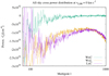 |
Fig. 2 Cross power spectra between WNM and CNM (PWxC), WNM and LNM (PWxL), and LNM and CNM (PLxC) at vLSR = 0 km s−1. |
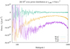 |
Fig. 3 Cross power spectra between WNM and CNM (PWxC), WNM and LNM (PWxL), and LNM and CNM (PLxC) at vLSR = 0 km s−1. |
3.2 Optical depth effects
The H I survey data we analyzed may suffer from optical depth effects. For the CNM the optical depth is expected to increase with decreasing spin temperature, though a general physically significant relationship cannot be established (Heiles & Troland 2003). An increase in the optical depth for the clumpy CNM can lead to a systematical underestimation of the observed column densities and this implies that the power at high multipoles is underestimated. In turn, observed power spectra may be steepened artificially.
We use an empirical correction derived by Lee et al. (2015) from Arecibo observations in direction to the Perseus molecular cloud which is consistent with data from Heiles & Troland (2003) and which was confirmed later by Murray et al. (2018a,b). Observed column densities NHobs are accordingly biased by a factor
 (5)
(5)
and we apply a correction NHcorr = f ⋅ NHobs for f > 1, this concerns CNM with NHobs≳0.6 × 1020 cm^-2. Using this correction we recalculate the power spectra for vLSR = 0 km s−1, as shown in Fig. 1. We find in all cases that power spectra for the CNM and the total H I get flatter. However, the resulting changes of the spectral indices are typically less than half of the rather low formal uncertainties of the fit. The spectral indices are within the errors unaffected by optical depth effects; only in one case do we find a slight change. In the case of the total all-sky H I column densities the index changes from γ = −2.776 ± 0.004 to γ = −2.768 ± 0.003. We conclude that optical depth effects cannot explain the observed steepening of the single-channel power spectra close to zero velocities. Optical depth effects are noticeable at high column densities in the Galactic plane. High latitude power spectra are essentially unaffected and we draw our conclusions predominantly from these data.
3.3 Power spectra for CNM, LNM, and WNM phase fractions
The power spectra discussed in Sect. 3.1 are caused by column density fluctuations of individual H I phases. Hence there are two effects competing with each other, fluctuations in column density and in phase composition. We want to determine power spectra merely related to individual H I phases, and therefore consider average phase fractions along the line of sight.
Phase fractions  depend in general on the velocity range and, following Kalberla & Haud (2018), for v1 < vLSR < v2 are defined as
 (6)
(6)
where Tb is the observed brightness temperature, while TbP stands for the brightness temperature contribution from phase P, P = CNM, LNM, or WNM. Since the dependences on column densities cancel in this expression, the weights for the decomposition into different phases are identical for all lines of sight. Derived multiphase power spectra are essentially deconvolved for column density effects. For a visualization of the spatial column density distributions for different phases in comparison to associated phase fractions, we refer to Kalberla & Haud (2018, Figs. 9 and 10).
In Fig. 4 we show power spectra from single-channel phase fractions at the velocity vLSR = 0 km s−1. Comparing the power spectra from Fig. 4 with those from Fig. 1 shows that now the spectra for all-sky and high latitudes are in far better agreement than before, but spectra for |b| > 20° are slightly steeper than the all-sky spectra. We observe significantly increased power at multipoles l≲lcrit. In the case of phase fractions the cosecant latitude effect of the Galactic disk is removed and possible biases (see Sect. 9) for low multipoles are minimized. The spectral indices for the phase fractions are − 1.8 > γ > −2.2 and are significantly flatter than − 2.14 > γ > −2.48 for the column density distributions discussed in Sect. 3.1. This flattening is most pronounced for the LNM and can be explained by the absence of column density fluctuations.
Phase fractions need to sum up to one, the bottom panel on the right side of Fig. 4 shows in the all-sky case the completely negligible power spectrum for deviations caused by the Gaussian decomposition (black). We note that this power spectrum now reflects the increased uncertainties at low multipoles from baseline uncertainties at the field boundaries discussed in Appendix A.2.3. The red curve shows apodization errors at high latitudes. They cause a considerable ringing, but fortunately such unavoidable errors are also not significant since they drop off very fast at high multipoles.
Phase fractions, defined by Eq. (6) are useful to study the gas composition independent from its total column density. These data do not represent any reasonable model for the multiphase H I distribution, but are useful to consider how strictly power spectra depend on the phase composition. Phase transitions cause shallow power spectra for l≲100 and enhanced power at higher multipoles.
4 Velocity dependent narrowband spectral indices
We consider now velocity dependences in the spectral indices. Figure 5 shows the average distribution of phase fractions for the local ISM at high latitudes in the velocity range − 16 < vLSR < 16 km s−1 (Kalberla & Haud 2018, Sect. 3). There are considerable fluctuations in the phase fractions and an imprint on the power distribution for individual phases at these velocities may be possible.
We consider first the model distributions of phase fractions that are unaffected by column density fluctuations. The velocity dependences of narrowband spectral indices for multipoles 10 < l < 100 are shown in Fig. 6 for all-sky and in Fig. 7 for |b| > 20°. We observe a general steepening of the spectral indices close to vLSR ~ 1 km s−1. The strongest effect is found for the CNM. The enhancement of the average CNM phase fraction at this velocity (Fig. 5) clearly leads to a pronounced steepening of the CNM power spectra. The steepening of the spectral indices of the other phases is noteworthy, but may be a consequence of the coupling of the power spectra between different phases according to Eq. (4).
Next we consider the power spectra derived from the Gaussian components of different H I phases. Figures 8 and 9 show still local minima for the CNM spectral indices, however the spectral indices for the other phases are now mostly anti-correlated; the WNM has a particularly smooth distribution. Spectral indices derived from power spectra of the total observed H I also show smooth changes. For high latitudes (Fig. 9, red) we find a steepening in anti-correlation to the WNM, but with local minima that are affected by the CNM and LNM. In the all-sky case (Fig. 8, black) we observe a smooth trend, but influences from the CNM and LNM are weak.
Velocity dependences for the spectral indices have been observed before (Kalberla & Kerp 2016; Kalberla et al. 2017). Recently, Choudhuri & Roy (2019) have presented data that show a steepening of the spectral indices at velocities that are considered to be representative for the CNM. Spectral indices for 13 CO (2–1) and 12CO (3–2) channel maps in the Perseus cloud were observed by Sun et al. (2006) with a steepening of the indices that can be described asan average structure of the index spectrum similar to the line profile.
Numerical studies of the condensation of WNM into CNM structures caused by turbulence and thermal instabilities were conducted by Saury et al. (2014). They found that turbulence plays a key role in the structure of the cold medium; it can induce the formation of CNM when the WNM is pressurized and put it in a thermally unstable state. They found evidence for subsonic turbulence with a shallow power index γ ~ −2.4. Recent high resolution simulations by Wareing et al. (2019) have shown that the thermal instability dynamically can form sheets and filaments on typical scales of 0.1–0.3 pc, explaining that as the structure grows in the simulation, the density power spectrum rapidly rises and steepens. Wareing et al. (2019; Fig. 10) derive γ ~ −3, but the steepening is most prominent on scales below 1 pc.
The preferred width of the filaments in the range 0.1–0.3 pc is consistent with unresolved cold small-scale structures observed by Clark et al. (2014) and Kalberla et al. (2016). Furthermore, these cold filaments have characteristic radial velocities close to zero km s−1. The single-phase power spectra show a strong increase at the corresponding multipoles l ~ 1023.
A steepening of thin velocity slice H I power spectra in a narrow velocity range, associated with a decrease in the WNM fraction and the coexistence of cold anisotropic CNM filamentary structures was reported before for three fields at intermediate latitudes by Kalberla et al. (2017; Sect. 6). The interpretation was that phase transitions, indicated by changes in H I phase fractions, modify the narrowband power distribution. For a determination of dependences between power spectra and phase transitions these authors proposed isolating particular cold H I components from the rest of the H I distribution in order to differentiate between ON velocities at the line centers and appropriate OFF velocities in the line wings. Accordingly we define here
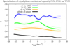 |
Fig. 8 All-sky velocity dependences of spectral indices for individual phases, and the total H I distribution (black). The thin lines represent the scatter for one-sigma uncertainties when the total H I distribution (black) uncertainties are within the thickness of the line. |
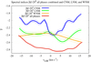 |
Fig. 9 High latitude velocity dependences of spectral indices for individual phases, and the total H I distribution (red). The thin lines represent the scatter for one-sigma uncertainties when the total H I distribution (red) uncertainties are within the thickness of the line. |
 (7)
(7)
as the power ratio and
 (8)
(8)
as the power excess, relating single-channel ON and OFF power distributions; POFF(l) is defined as the average single-channel power at two OFF positions.
The choice of the ON velocity is obvious, we observe at vLSR = 3 km s−1 the highest CNM and at the same time the lowest WNM ratio (Fig. 5). The high latitude data also show at this velocity a well-defined minimum for the CNM spectral index (Fig. 9). From this plot the definition for the OFF velocities at vLSR = 3 ± 5 km s−1 is also well defined, the CNM power law steepening is limited to the range ΔvLSR ~ 10 km s−1; we refer to Sects. 5.3–5.6 for further discussion of the velocity spread.
Figure 10 shows the power ratios ℜ(l). We observe ℜ(l)≳1 for all multipoles except l ~ 30. For the WNM ℜ(l) is flat but LNM and CNM show enhancements at high multipoles. Strong fluctuations are also observable at multipoles 10≲l≲50.
Figure 11 shows the power excess 𝔈 (l). In comparison to Fig. 1 (γ = −2.776 ± 0.004 for the total H I and γ = −2.37 ± 0.03 for the CNM) we observe steep power spectra with γ = −2.87 ± 0.02 for the total H I for l≳10, and in particular γ = −2.8 ± 0.1 for the CNM for 10≲l≲100. This is by far the steepest power law derived by us for the CNM, and we interpret the steep excess power distribution 𝔈 (l) for the CNM asinduced by phase transitions. Thermal instabilities obviously also affect the power spectra for WNM and LNM; they are no longer straight, but bent up systematically with increasing power for high multipoles. The different phases are correlated according to Eq. (4), but the power spectrum for the total H I remains straight.
In agreement with Kalberla et al. (2017) we find strong evidence that the power distribution in the local ISM issignificantly steepened by phase transitions. The CNM is filamentary and anisotropic on small scales (Kalberla & Kerp 2016; Kalberla et al. 2017), but even the large CNM power ratios ℜ(l) at low multipoles appear to be linked to large-scale filaments, oriented along the magnetic field as observed by Clark et al. (2014) and Kalberla et al. (2016).
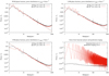 |
Fig. 4 Power distributions for phase fractions in different H I phases at vLSR = 0 km s−1. Top left: WNM; top right: LNM; bottom left: CNM. Black lines show all-sky data, red lines are for |b| > 20°. Spectral indices are derived at 10 < l < 100 as indicated by the vertical lines. Bottom right: uncertainties from the Gaussian decomposition (black) and ringing caused by apodization (red). |
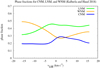 |
Fig. 5 Velocity distribution of average H I phase fractions for CNM, LNM, and WNM using unpublished data from Kalberla & Haud (2018). |
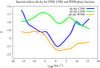 |
Fig. 6 All-sky velocity dependences of spectral indices for H I phase fractions. The thin lines represent the scatter for one-sigma uncertainties. |
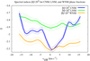 |
Fig. 7 High latitude velocity dependences of spectral indices for H I phase fractions. The thin lines represent the scatter for one-sigma uncertainties. |
 |
Fig. 10 Power ratio ℜ(l) according to Eq. (7). The ON velocity is vLSR = 3 km s−1; OFF is calculated as the average of single-channel slices at vLSR = −3 and 7 km s−1. The dotted line indicates ℜ(l) = 1. |
 |
Fig. 11 Power ratio 𝔈(l) according to Eq. (8). The ON velocity is vLSR = 3 km s−1; OFF is calculated as the average of single-channel slices at vLSR = −3 and 7 km s−1. The spectral index for the total HI is calculated for l > 10; in the case ofthe CNM for 10 < l < 100, the horizontal lines indicate these limits. |
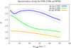 |
Fig. 12 All-sky dependences of spectral indices for H I phase fractions and velocity channel width. The thin lines represent the scatter for one-sigma uncertainties. |
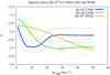 |
Fig. 13 Dependences of spectral indices for H I phase fractions and velocity channel width at |b| > 20°. The thin lines represent the scatter for one-sigma uncertainties. |
5 Spectral indices and velocity channel widths
In this section we determine spectral indices for individual H I phases after integrating the column density distributions over several channels with a total full width at half maximum (FWHM) of ΔvLSR. Figures 12 and 13 show the results. From the all-sky data we note that the spectral indices for WNM and LNM steepen continuously. The WNM has broad lines, resulting in a slow change in spectral index. The characteristic LNM line widths are narrower, corresponding to faster changes of the slope with ΔvLSR. For the CNM the situation is more complex. In the case of the all-sky data we note a prominent minimum at ΔvLSR = 5 km s−1 and a rise afterward. At high latitudes the situation is similar, but the CNM spectral index now has a broad minimum around ΔvLSR ~ 10 km s−1.
From the observed H I column densities or the sum of all phases we derive the spectral indices shown in Fig. 14. Spectral indices decrease in a similar way for the all-sky data and for |b| > 20° until ΔvLSR = 16 km s−1. Afterward the indices diverge; they fall for all-sky data but rise for |b| > 20°. This result is unexpected, and an explanation is needed.
 |
Fig. 14 All-sky dependences of spectral indices for observed H I column densities as a function of the velocity channel width. The thin lines represent the scatter for one-sigma uncertainties. |
5.1 Velocity channel analysis
Power spectra extracted from narrowband data (thin velocity slices) are affected by turbulence in two ways. Density fluctuations have an imprint on the observed column densities, but velocity fluctuations also need to be taken into account. To separate effects caused by fluctuations in density or velocity, the basic idea of VCA is to increase the width ΔvLSR of the velocity slice. Velocity fluctuations should average out, and when the velocity window ΔvLSR is broad enough that all internal velocities are covered (thick velocity slice) the observed emissivity should eventually be dominated by density fluctuations Lazarian & Pogosyan (2000; Eq (25)). The expected minimum velocity width is ΔvLSR ~ 17 km s−1 Lazarian & Pogosyan (2000; Sect. 4.3), the typical FWHM thermal line width for the WNM. Starting with a thin velocity slice and successively increasing the velocity width, a gradual steepening of the spectral index should be observed until convergence. For our application to H I column densities we observe a steepening (Fig. 14), but in the case of high latitude data only until ΔvLSR ~ 16 km s−1, which is the maximum linewidth for consistent results. Considering the CNM in Figs. 12 and 13 we find a steepening, but subsequently the spectral index flattens again. The question arises whether VCA is applicable to our data. We take up the discussion later in Sect. 7.
Spectral indices close to γ ~−2.95 and within the uncertainties of Δγ≲0.1 independent of velocity widths 0.82< ΔvLSR < 21.4 km s−1 have been reported by Khalil et al. (2006; Tables 3 and 4, Fig. 29). A constant spectral index is inconsistent with VCA; these authors discuss in their Sect. 6 some other observations that do not show the steepening predicted by VCA. Yuen et al. (2019) note that the analysis of the data agrees well with VCA predictions and revise the Khalil et al. (2006) indices in their Table 3 to γthin = −2.6 and γthick = −3.4. No details are given how this result was obtained, but the authors refer to a forthcoming more detailed paper.
5.2 Velocity channel cross-correlations
Trying to better understand the dependences between turbulent power distribution and the velocity window width ΔvLSR, we calculate cross-correlations for single-channels in the wings of the line signal. Hence we cross-correlate channels separated by a distance ΔvLSR in velocity. This is a differential approach. The cross power spectra that we use to study internal velocity dependences of individual H I phases are, according to the Wiener-Khintchine theorem, the Fourier transforms of the cross-correlation function at particular characteristic lags in velocity. In the case of a signal from a genuine turbulent medium, the cross power spectra should inform us on how well correlated the individual H I phases remain throughout their velocity distribution.
We consider high latitudes first; all-sky data is deferred until Sect. 5.8. Figure 15 shows us the cross-correlations between two channels at velocities vLSR = −5 km s−1 and vLSR = +5 km s−1. For the WNM we find a well-defined power spectrum with a slope of γ = 2.41 ± 0.06 for multipoles 10 < l < 100 with enhanced power at high multipoles. For the LNM no power law can be found for 10 < l < 100 (only positive values of Cl can be plotted), but for this phase we also obtain enhanced power at high multipoles; the velocity cross power distributions for LNM and WNM are almost identical there. In the case of the CNM only a noisy cross-correlation signal at high multipoles can be seen. In comparison to the expected contribution of the uncertainties from the Gaussian decomposition shown in Fig. 1 this signal (~1030 cm−4) is barely significant. The local minimum of the spectral index for the CNM phase in Fig. 15 at ΔvLSR = 10 km s−1 indicates that the correlation of the CNM is lost. This implies that on average any CNM structure seen in channels separated by ΔvLSR≳10 km s−1 is unrelated. Homogeneous CNM clouds have an average FWHM line width of 3.6 km s−1 (Kalberla & Haud 2018) and according to Sect. 5.5 only 3.2 km s−1 for velocities |vLSR|≲5 km s−1. The internal velocity distribution of individual CNM clouds is too narrow to cause a limitation of this kind. The implication must be that CNM clumps in a turbulent flow decouple from each other if their center velocities differ by  km s−1. In the following we investigate this remarkable result further; in Sect. 6 an explanation is offered from constraints considered by Kolmogorov (1941). Both the WNM and LNM maintain their correlation at a lag of 10 km s−1. Their cross power spectra are identical for l≳200; in Fig. 13 the LNM data overplot the WNM data. Increasing the velocity separation for two channels further, we also observe for the LNM a decorrelation of the cross power for ΔvLSR≳26 km s−1. This is discussed later in Sect. 5.4 and demonstrated in Fig. 19.
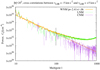 |
Fig. 15 Cross-correlations at latitudes |b| > 20° between two channels at vLSR = −5 and vLSR = +5 for the WNM, LNM, and CNM. |
5.3 Constraints on spectral coherence
A different way to explore correlations in the velocity domain is by defining the spectral coherence Sl (v1, v2) between two single channels at velocities v1 and v2
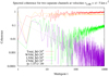 |
Fig. 16 Spectral coherence for velocity slices at vLSR = −5 km s−1 and vLSR =+5 km s−1 for the total H I, WNM, LNM, and CNM. |
![Mathematical equation: \begin{equation*} S_l(v_1,v_2) = C_l^2 (v_1,v_2) / [ C_l(v_1,v_1) \cdot C_l(v_2,v_2) ],\end{equation*}](/articles/aa/full_html/2019/07/aa34533-18/aa34533-18-eq12.png) (9)
(9)
where Cl(v1, v2) is the cross-correlation between individual PPV channel maps at velocities v1 and v2 with corresponding autocorrelations Cl(v1, v1) and Cl(v2, v2). This relation has the advantage that it is independent of beam smoothing as long as the H I emission is little affected by noise. It is clear that Sl = 1 for v1 = v2 and the signal decorrelates for increasing channel separation, but we require for a turbulent flow that some correlation should be maintained if we want to define eddies as coherent patterns of flow velocity, vorticity, and pressure.
We use high latitude data to calculate Sl(v1, v2) for the WNM, LNM, CNM, and the total H I column density distributions at velocities v1 = −5 km s−1 and v2 = +5 km s−1. The results are shown in Fig. 16. The WNM distribution is coherent at all multipoles l. This is expected since the velocity spread v2 − v1 = 10 km s−1 is small compared to the average FWHM width of 23.3 km s−1 of the WNM emission (Kalberla & Haud 2018). In the case of the LNM with an average FWHM 9.6 km s−1 some spectral coherence remains at high multipoles. This behavior is expected for an unstable phase that is embedded in the WNM, but surrounds a clumpy CNM distribution (see Sect. 5.7). For the CNM with an average FWHM width of 3.6 km s−1 the fit γ = −1.07 ± 0.09 at a channel separation of ΔvLSR = 10 km s−1 is within the uncertainties consistent with random Gaussian noise (γ = −1). For comparison, the spectral coherence is also shown for the total multiphase H I column density (Fig. 16, red). This is expected close to one, but interestingly the scatter in Sl is large compared to the WNM. Clearly the WNM derived from Gaussian components provides a more consistent presentation of the large-scale H I distribution.
We repeat the calculations and determine Sl for v2 − v1 < 10 km s−1; coherence for the CNM is recovered. As an example we use Sl (v1, v2) for v1 = −2 km s−1 and v2 = +2 km s−1. This velocity lag corresponds roughly to the average FWHM width of 3.6 km s−1 for the CNM. The result is shown in Fig. 17. For the WNM the situation is similar to Fig. 16, but for the CNM we find coherence for l > 100. This situation can be described as follows: power in the CNM exists spatially predominantly on small scales, and structures in velocity space can only be detected for small velocity lags. Increasing the velocity lag leads to a gradual decorrelation; as shown in Fig. 16, the spectral coherence is lost completely for ΔvLSR = 10 km s−1; the CNM inthe two separate channels decouples if this value is exceeded.
For the LNM we find correlation on larger scales (up to smaller multipoles) and at the same time for larger velocity lags. The LNM surrounds the CNM, occupying a larger volume and at the same time a larger velocity spread. Some evidence for this hierarchical structure was given before by Kalberla & Haud (2018). Increasing the lag v2 − v1 we find a gradual decorrelation for the LNM, the LNM decouples for ΔvLSR≳23 km s−1.
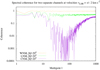 |
Fig. 17 Spectral coherence for velocity slices at vLSR = −2 km s−1 and vLSR =2 km s−1 for the WNM, LNM, and CNM. |
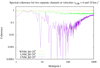 |
Fig. 18 Spectral coherence for velocity slices at vLSR = 6 km s−1 and vLSR =10 km s−1 for the WNM, LNM, and CNM. |
5.4 Self-similarities in velocity space
The missing correlation between CNM clouds with velocity lags δvLSR≳10 km s−1, and the good spectral coherence of the CNM at lags δvLSR ~ 4 km s−1 shown in Fig. 17 do not imply that the CNM distribution is restricted in velocity space. The CNM can exist independently at other bulk velocities (v1 + v2) ∕ 2 and other domains embedded in LNM.
To demonstrate this we repeat the calculations and determine Sl (v1, v2) for v1 = 6 km s−1 and v2 = 10 km s−1. The result is shown in Fig. 18 and resembles the CNM in Fig. 17. The local H I is self-similar concerning the properties of the phase distribution in velocity space even though the column densities are significantly different at vLSR ~ 0 and vLSR ~ 8 km s−1. Differences in phase fractions (Fig. 5) and spectral indices (Figs. 7 and 9) also exist, but they have no significant imprint on the spectral coherence of the CNM. For the LNM we find in comparison to Fig. 17 an increase in spectral coherence at multipoles l≲100, caused by the reduced contribution of CNM to the H I at velocities δvLSR ~ 8 km s−1.
Self-similarities are also recognizable for the LNM though the velocity limits are in this case less sharply defined than in the case of the CNM. Figure 19 shows examples of lags between velocities v = −15, 0, and 15 km s−1. The spectral coherence inthe LNM is lost at large velocity lags, but can be recovered by gradually decreasing the width of the velocity lag, independent of the bulk velocity (v2 + v1)∕2. The example in Fig. 19 also shows that the spectral coherence values for the LNM at negative and positive bulk velocities are comparable, while slight differences exist for the WNM.
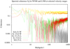 |
Fig. 19 Spectral coherence Sl(v1, v2) for WNM and LNM velocity slices. The labels indicate the velocities v1 and v2 and the phases, WNM (W) or LNM (L). |
5.5 Spectral coherence at high multipoles
The dependence of Sl(v1, v2) (Eq. (9)) on the lag Δv = v2 − v1 can be best studied at high multipoles. We consider vLSR = (v2 + v1) ∕ 2 = 0 km s−1 and use high latitude data at |b| > 20°. To suppress random fluctuations we average Sl(v1, v2) for l≳1000. The results are shown in Fig. 20 with symbols. We try to model these Sl distributions by assuming that they are caused by a sample of H I clumps with characteristic Doppler temperatures and corresponding Gaussian line shapes. This works well for the CNM, but fails in the case of the LNM. For the CNM we fit a FWHM width of 3.20 ± 0.01 km s−1; this Gaussian is shown in Fig. 20. For comparison we plot for the LNM a Gaussian with FWHM width of 10 km s−1. It is obvious that the LNM cannot be approximated by a Gaussian distribution with a single characteristic line width. This implies that the CNM and the LNM must have very different properties. The CNM can be described as a phase that occupies a well-defined range in velocity width. The LNM as an unstable phase may be “best understood as a range of density and temperature values” (Vázquez-Semadeni 2012). A large scatter in Doppler temperatures (or line widths) observed by Kalberla & Haud (2018, Fig. 7) supports this proposal. The missing stability of the LNM implies that H I gas in this phase has to develop either to CNM or to WNM; the line width distribution gets stretched out in both directions.
The fitted CNM line width of 3.20± 0.01 km s−1 corresponds to a Dopplertemperature of TD = 223.7 ± 2 K. This temperature was reported previously by Kalberla et al. (2016) for cold filamentary H I gas. The agreement is at first glance surprising since filamentary structures, derived from unsharp masking (USM), have typically low column densities. Kalberla & Haud (2018) determined an average CNM line width of 3.6 ± 0.1 km s−1, corresponding to a Doppler temperature of 283 K, from profiles with less than eight well-defined Gaussian components. They assumed that the Gaussian analysis would recover only a part of the weak components. The cold filamentary USM structures, however, turn out to be characteristic of the small-scale structure of the CNM if velocities are restricted to the velocity range − 5< vLSR < 5 km s−1.
Unsharp masking aims to extract H I structures at the highest spatial frequencies that can be observed by large single-dish radio telescopes. The Doppler temperature was determined by Kalberla et al. (2016) as the median and also by fitting a log-normal probability density distribution5. Here we select coherent structures at high multipoles and derive the column density weighted geometrical mean Doppler temperaturefrom the correlation functions. The methods for both investigations are quite different, in each case with uncertain assumptions, but the resulting Doppler temperatures agree very well.
A characteristic temperature for the CNM can also be derived directly from the sample of Gaussian components. From narrowband data at high Galactic latitudes with δvLSR = 1 km s−1 we derive the lowest median TD = 208 K at vLSR = 0 km s−1. For the velocity range − 5< vLSR < 5 km s−1 we obtain a median TD = 217 K and a mean TD = 229 K. These TD values are deconvolved for the instrumental line broadening caused by the spectrometers and agree well with the value TD = 223.7 ± 2 K, derived by fitting Sl. No deconvolution is necessary for Sl determined from Eq. (9) because bandwidth and beam effects cancel in this case. Thus, the median Doppler temperature TD = 223 K for small-scale CNM structures is well defined and confirmed by our current investigations.
Extracting prominent cold filaments (Kalberla et al. 2016) is equivalent to selecting H I components with steep spectral indices (see also Sect. 4). A completely independent determination of H I small-scale structures with the Arecibo telescope by Clark et al. (2014) leads, within the errors, to the same result; these authors found a Doppler temperature of 220 K. Clark et al. (2019) have proven recently that anisotropic magnetized H I small-scale structures and narrow linewidths are dust-bearing density structures. They found that anisotropic small-scale H I channel map structures are correlated in position and position angle with far infrared structures at 857 GHz, implying that this emission originates from a colder, denser phase of the ISM than the surrounding material.
Coherent CNM structures, described by Sl according to Eq. (9), can be interpreted as eddies (see Clark et al. 2014, Figs. 3 and 4, or Kalberla & Kerp 2016, Figs. 28 and 29). These structures are caused by a well-defined population of CNM clouds with characteristic log-normal distributions in column density and Doppler temperature (Kalberla & Kerp 2016, Figs. 12 and 13). The properties of these CNM structures are well defined. They are cold, dusty, magnetized, and aligned with the local magnetic field (Clark et al. 2014, 2019). Typical temperatures of the associated dust are Tdust ~ 18.5 K. These structures are embedded in LNM with Tdust ~ 19 K (Kalberla & Haud 2018). Anisotropies associated with radio-polarimetric filaments, explored by Kalberla & Kerp (2016) and Kalberla et al. (2017), suggest that these structures are shaped by MHD turbulence in the presence of a magnetic field (Goldreich & Sridhar 1995). Filamentary features from these observations are probably mostly sheets with systematic velocity gradients perpendicular to the field direction. According to Heiles & Crutcher (2005), “edge-on sheets should be edge-on shocks in which the field is parallel to the sheet”. Not all of the data can be explained this way. An alternative interpretation of filaments as fibers, having an approximately cylindrical geometry, was given by Clark et al. (2014).
A characteristic Doppler temperature of 223 K implies for an average spin temperature of 50 K (Heiles & Troland 2003) a mean Mach number of M ~ 3.8 for the CNM, a value that agrees well with the estimate of M ~ 3.7 by Heiles & Troland (2005). Using a median spin temperature of 61–79 K (Murray et al. 2018b, Table 4) would result in 2.8≲M≲3.3.
According to Lazarian & Pogosyan (2000) small-scale structures in the H I do not reflect masses of real clumps, but are caustics produced by the turbulent velocity field via projection; this process is also called velocity mapping (Lazarian & Pogosyan 2000, Sect. 6). Observational parameterized structures with properties as summarized in the last two paragraphs were newly rejected as being real entities. Lazarian & Yuen (2018) conclude that “the filaments observed by Clark et al. (2014) in thin channel maps can be identified with caustics caused by velocity crowding”. Clark et al. (2019) object and conjecture instead that “small-scale structures in narrow H I channel maps are preferentially cold neutral medium that is anisotropically distributed and aligned with the local magnetic field”. We also interpret these structures as density enhancements, CNM eddies from a turbulent flow, caused by phase transitions and observable at the resolution limit of large single-dish telescopes. Phase transitions may be partly provoked by turbulence (Saury et al. 2014), but cause at the same time back-reactions on the power distribution (see also Sects. 4 and 7.4).
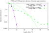 |
Fig. 20 Dependences of the spectral coherence Sl(v1, v2) on the lag Δv = v2 − v1 for the CNMand LNM at |b| > 20°. Averages for multipoles l < 1000 are given (points) in comparison with Gaussian distributions with FWHM widths of 3.2 and 10 km s−1 (lines). |
5.6 Linewidth regimes for different phases
The FWHM velocity window width for the steepest CNM power index (Fig. 13) is identical with the lag where spectral coherence for the CNM is lost. This velocity window is also identical with the mean LNM line width of 9.6 km s−1 determined by Kalberla & Haud (2018). The model assumption of the LNM as a transition between the stable clumpy CNM and diffuse WNM implies that the velocity space covered by the LNM must be at least as large as the velocity spread where we find coherence inthe CNM. The LNM is unstable, and there is a high probability of finding it associated with CNM, which causes a coupling between both phases in velocity space.
By generalizing such a hierarchical scheme in the velocity space, we assume that the spectral power for the LNM distribution, which is also embedded in the WNM, should be correlated with the mean FWHM velocity width of 23.3 km s−1 for the WNM (Kalberla & Haud 2018). Figure 13 shows that this is the velocity width of the steepest LNM spectral index. For broader velocity windows the LNM spectral index is flattening since the correlation between channels separated by ΔvLSR≳23 km s−1 is lost.
We conclude that the mean FWHM velocity widths of the different phases are not independent from each other; instead, they reflect correlations between the H I phases. Saury et al. (2014) report from their simulations “that the turbulent motions inside clumps and the relative velocities between them are related to the motions of the WNM from which they were formed”, which means that “a non-negligible fraction of the measured velocity dispersion is caused by the relative motions of the clumps along the line of sight, suggesting that the observed line broadening is likely to be due to the relative clumps motions rather than supersonic turbulence”.
5.7 Spatial phase coherences
To study the spatial relationship between different phases we define, in analogy to Eq. (9), the spatial phase coherence
![Mathematical equation: \begin{equation*} P_l(\mathrm {A,B}) = C_l^2 (\mathrm {AxB}) / [ C_l(\mathrm {AxA}) \cdot C_l(\mathrm {BxB)} ],\end{equation*}](/articles/aa/full_html/2019/07/aa34533-18/aa34533-18-eq13.png) (10)
(10)
between phases A and B. Here Cl(AxB) is the cross-correlation between PPV channel maps for phases A and B, and Cl (AxA) denotes the auto correlation for phase A, and Cl(BxB) for phase B. A and B stand for CNM, LNM, and WNM; Pl depends in general not only on the H I phases, but also on the velocity range v1, v2.
Figure 21 shows Pl for single channels at vLSR = 0 km s−1. Here Pl(CNM, LNM) indicates that the CNM is dominating high multipoles l≳100; Pl (LNM, WNM) shows that the LNM is somewhat more extended with l≳50; Pl (CNM, WNM) indicates that CNM and WNM are spatially almost uncorrelated since the LNM is enveloping the CNM, see also Fig. 3. Within the noise a very weak correlation Pl(CNM, WNM) remains; this signal is noisy because of the low volume filling factor of the CNM. To find a relation between CNM and WNM it is necessary toconstrain the statistics by selecting positions with a significant phase fraction for the CNM (see Kalberla & Haud 2018).
The spatial phase coherence Pl is self-similar for changes in bulk velocity (v1 + v2) ∕ 2 and velocity spread v2 − v1 as long as the spectral coherence for the individual H I phases is not violated.
5.8 Galactic plane data – differential Galactic rotation
Next we consider the all-sky data shown in Fig. 14. Due to the strong emission in the Galactic plane, the all-sky cross-correlations for channels with a separation of ΔvLSR = 26 km s−1 (see Fig. 22) are significant for WNM, LNM, and the sum of all phases. However, what we observe is not a signal that we expect for a genuine turbulent flow. The observed H I column density distribution in the Galactic plane is affected by differential Galactic rotation, causing at Galactic longitudes Glon a sin (2 ⋅ Glon) modulation (e.g., Mebold 1972). In particular, velocities close to zero are affected by velocity crowding (Burton 1972), leading to a systematic degradation of the signal for l≲100; the assumption of homogeneity and isotropy is no longer valid. High column densities from the Galactic plane dominate the statistics. Checking cross-correlation spectra with smaller velocity separation we can trace this problem to channel separations as low as ΔvLSR = 16 km s−1. HI4PI all-sky data, in short, are affected by confusion from the Galactic plane, and are therefore only of limited use to us.
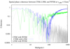 |
Fig. 21 Single-channel spatial coherences Pl at vLSR= 0 km s−1 for CNM, LNM, and WNM. |
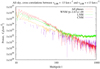 |
Fig. 22 All-sky cross-correlations between vLSR = −13 and vLSR = +13 for the totalH I, WNM, LNM, and CNM. |
6 Kolmogorov’s local constraint
Kolmogorov (1941) constrained his paper on “turbulence in incompressible viscous fluids for very large Reynolds numbers” to locally homogeneous and isotropic structures. The term “locally” was (except for stationarity in time) specified by Kolmogorov as “restrictions are imposed only on the distribution laws of differences of velocities and not on the velocities themselves”.
A remarkable result of our investigations in Sects. 4 and 5 is that the properties of the turbulent flow in the multiphase ISM are limited concerning velocity differences (lags (v2 − v1) used by us). For the two phases, CNM and LNM, we find a decorrelation of the flow in velocity (Fig. 15) and describe this phenomenon as a loss in spectral coherence (Fig. 16). The decorrelation depends on spatial properties of the flow. The CNM dominates high multipoles l≳100 (Fig. 17), and decorrelation happens at lags v2 − v1 ~ 10 km s−1. The LNM exists at multipoles l≳50 (Fig. 21) and decorrelates at lags v2 − v1 ~ 23 km s−1. Thus, for both phases we have well-defined domains, and in agreement with Kolmogorov (1941) “the hypothesis of local isotropy is realized with good approximation in sufficiently small domains G of the four-dimensional space”. We find self-similarities, i.e., the properties of the CNM and LNM do not change significantly when shifting the velocities (Figs. 18 and 19), but decorrelation at large velocity differences remains, independent of the “velocities themselves” that are investigated. Turbulence in the local ISM is locally constrained but otherwise is homogeneous and isotropic (for a comparison between the power spectra from two hemispheres, see the lower right panel of Fig. A.2).
Restricting turbulence to be locally constrained, Kolmogorov (1941) probably also had limitations from the experimental setup in mind; the domain under investigation should not be “lying near the boundary of the flow or its other singularities”. Except for the layered structure of the H I, affecting according to Sect. 9 multipoles l≲9, and apodization to avoid confusion from the Galactic plane, our investigations are not affected by boundaries. Our global panoramic view is based on a coordinate system that is comoving with the LSR in the center of a locally turbulent flow and should not generate limitations concerning “velocity differences”.
7 VCA revisited
With the results from Sect. 5 we now apply a modified velocity channel analysis (Lazarian & Pogosyan 2000) to our data. From the theoretical point of view VCA is quite appealing; however, from the channel cross power analysis in the previous section we see that some care is needed to avoid biases caused by a decorrelation of the H I database due to confusion that is, unfortunately, not easily recognizable from the data. From the multiphase composition of the ISM we get additional constraints that are also not recognizable without a decomposition in different phases.
7.1 Characteristic broadband spectral indices
We conclude from Fig. 14 that the best possible estimates for multiphase broadband power spectra in our case should be derived for ΔvLSR = 16 km s−1. This is rather narrow compared to the typical FWHM width of 23.3 km s−1 for the WNM, but interestingly this width is close to the FWHM width of ΔvLSR = 16.8 km s−1 for the velocity distribution of filamentary H I structures. It has been suggested that these structures indicate processes that feed kinetic energy to the local ISM (Kalberla et al. 2016, Sects. 5.13 and 5.14, Fig. 22). We show the broadband spectral distributions resulting for ΔvLSR = 16 km s−1 in Fig. 23, and obtain remarkably well-defined results: γ = −2.943 ± 0.003 for all-sky and γ = −2.944 ± 0.005 for high latitudes. The derived uncertainties are formal one-sigma errors, but systematic fluctuations on the order of Δγ ~ 0.05 may be more characteristic.
Decomposing broadband distributions for individual phases leads, according to Fig. 23 for multipoles 10 < l < 100, to all-sky spectral indices − 2.15 > γ > −2.5, comparable to the single-channel results at vLSR = 0 km s−1, shown in Fig. 1. These results are questionable since they may be affected by spurious effects from differential Galactic rotation. At high latitudes we obtain γ = −2.40 for the WNM and γ = −2.48 for the other phases. These values differ only slightly from the single-channel result γ ~ −2.36 at vLSR = 0 km s−1. The cross power spectral index for the WNM at high latitudes with a channel separation of vLSR = 10 km s−1 (Fig. 15) is, within the errors, identical to the auto power WNM spectral index γ = −2.40 for ΔvLSR = 16 km s−1 (Fig. 23).
At high Galactic latitudes the spectral indices for broadband power spectra may also be determined from Fig. 13, assuming that for single H I phases the minima of the derived distributions are more characteristic. We obtain in this case for CNM and LNM γ ~−2.5; the value for the WNM also appears to be consistent with this result, though a minimum is not yet reached at ΔvLSR = 50 km s−1. All-sky results according to Fig. 12 cannot be used this way; these data are obviously affected by confusion.
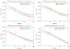 |
Fig. 23 Power distributions for different H I phases at − 8 < vLSR < 8 km s−1. Top left: WNM; top right: LNM; bottom left: CNM; and bottom right: sum of all phases with uncertainties from the Gaussian decomposition (cyan and orange). Black lines show all-sky data; red lines are for |b| > 20°. Spectral indices γ for CNM, LNM, and CNM are derived at 10 < l < 100 for the sum of all phases at l > 8, as indicated by the vertical lines. |
7.2 Modified VCA spectral index for the density field
The observational determined 3D spectral index γ, according to Lazarian & Pogosyan (2000) or Lazarian (2009, Table 3), can be used to estimate the spectral index of the density correlation function Γρ and for the velocity correlation function Γv, respectively. For data that are averaged over velocity the observed fluctuations in column density must be due to density fluctuations. In the case of a shallow 3D density distribution with Γρ > 0 the observed thick slice power index corresponds to γ = −3 + Γρ > −3; this transformation is essentially a reduction in dimensionality.
Not foreseen in the framework of VCA are limitations due to a decorrelation of the velocity field. We use for CNM and LNM the minima of the spectral index distribution from Fig. 13, both close to γ = −2.5. This value also appears reasonable for the WNM. We obtain Γρ ~ 0.5. Using indices from Fig. 23 would result in Γρ ~ 0.6 for the WNM and Γρ ~ 0.52 for LNM and CNM. We disregard all-sky data since they are most probably biased by confusion from the Galactic plane. Using observed H I column densities with a 3D spectral index γ ~−2.94 (Fig. 23 bottom right) would imply Γρ ~ 0.06. Given all the constraints discussed previously we consider this value (or γ ~−2.94 for the 3D density field) as characteristic of the total H I gas phase, but unrelated to the multiphase composition.
7.3 Modified VCA spectral index for the velocity field
For thin velocity slices in the case of a shallow 3D density distribution with γ > −3, the observed power index corresponds to γ = −3 + Γρ + Γv∕2 (Lazarian 2009, Table 3). Here Γv is the spectral index of the velocity correlation function. For this relation it is assumed that intensity fluctuations in thin velocity slices are significantly affected by velocity effects. Line emission that is shifted in velocity can mimic density fluctuations, so-called caustics. OnGalactic scales this effect is known as velocity crowding (Burton 1972). For shallow density spectra (i.e., γ > −3) and independent random velocity and density distributions, the pure velocity effect should dominate the density fluctuations on large scales (Lazarian & Pogosyan 2006), where fluctuations are supposed to be large compared to the mean density. Lazarian & Yuen (2018) conclude that on scales larger than 3 pc, corresponding to multipoles l≲100 at an assumed distance of 100 pc, fluctuations in channel maps are dominated by velocity fluctuations. Thus, velocity caustics should mimic real physical entities such as filaments. Clark et al. (2019) reject this interpretation and find that the H I intensity features are real density structures in a multiphase medium and not velocity caustics. Cold CNM filamentary structures exist predominantly at small scales, or l≳100, and should (at least for shallow H I power spectra) be largely unaffected by velocity fluctuations.
Thus, according to Lazarian & Pogosyan (2000) and Lazarian (2009) Γv ∕2 can be determined from changes between thin and thick velocity slice power distributions. We use results at high latitudes shown in Fig. 13 and find changes in the power law index in the range 0.12 to 0.16. Accordingly, we estimate Γv ~ 0.28 for the individual H I phases. In the case of total H I column densities we obtain from Fig. 14, Γv ~ 0.3. These results are low in comparison to the Kolmogorov (1941) index Γv = 2∕3, but intermittency and supersonic motions may modify this index (Kolmogorov 1962). For a compressible ISM the spectral indices may depend on the sonic Mach number (e.g., Burkhart et al. 2010). A 3D spectral index of γ ~ −2.5 for 10≲l≲100 implies accordingly Mach numbers near eight, though from the Gaussian decomposition lower values are expected: MCNM = 4.4, MLNM≲3.6, and MWNM ~ 1.4 (Kalberla & Haud 2018).
Our estimates of Γv according to a modified VCA are lower limits only. The HI4PI survey data are limited in velocity resolution to δv = 1 km s−1 for GASS and δv = 1.5 km s−1 for EBHIS, the asymptotical thin slice limit is not reached. At ΔvLSR = 0 km s−1 we should see in Figs. 12 and 13 a horizontally tangential approach. Our resolution is insufficient to derive a significant thin slice velocity limit. The demanding condition δv ≪ 1 km s−1 for a narrow line width is quite a surprise since the estimate by Lazarian & Pogosyan (2000, Sect. 4.3) was that a thin slice of δv ~ 2.6 km s−1 should be a sufficient velocity slice width for the H I. Very thin slices in velocity may cause serious observational problems; the instrumental noise would be significantly increased and the noise term Nl then needs to be explicitly taken into account.
7.4 Phase transitions versus velocity caustics
In the previous subsection we derived VCA predicted spectral index changes with constraints on spectral coherence from Sect. 5. Here we explore how the VCA solution depends on multipole l. In particular we want to derive how much the CNM power distribution PCNM(l) is modified by bandwidth changes ΔvLSR in velocity. We define the ratio
 (11)
(11)
for the narrowband (single-channel) power Pnarrow(l) and broadband power Pbroad(l), integrated over the CNM coherence width ΔvLSR = 10 km s−1, both at identical center velocities.
We chose two velocity settings. In the first case, for vLSR = 0 km s−1, there are significant fluctuations in the CNM spectral index. The second velocity, vLSR = −10, was chosen such that the CNM spectral index has little fluctuations (see Fig. 9). We show ℜVCA(l) for vLSR = 0 km s−1 in Fig. 24 and for vLSR = −10 in Fig. 25. In each case we observe more power than expected from the increased bandwidth, ℜVCA(l) > 10. There are inaddition two multipole ranges with different slopes in log–log presentation.
For l≲100 we observe a steepening of the spectral index with δγ = −0.12 ± 0.04 at vLSR = 0 km s−1 (Fig. 24) and δγ = −0.21 ± 0.04 at vLSR = −10 km s−1 (Fig. 25). This steepening is expected from the velocity correlation function (Lazarian & Pogosyan 2000; Lazarian 2009), and we derive accordingly Γv ~ 0.24 at vLSR = 0 km s−1 and Γv ~ 0.4 at vLSR = −10 km s−1, consistent with the results from the previous subsection.
For l≳100 we observe the opposite trend, i.e., the power increases for high multipoles. The sign for δγ is positive, but the distribution cannot be approximated with a constant spectral index. Could this multipole range be biased? According to Lazarian & Pogosyan (2000) the velocity slice thickness must be increased to steepen the power law distribution; however, this approach leads to contradictions. For an increase in slice thickness beyond ΔvLSR ~ 10 km s−1 we observe for low mutilpoles a flattening of the spectral index (see Sect. 5, Fig. 13). The power at high multipoles increases further. Thepower for l≳100 cannot be explained as being caused by velocity caustics. It must originate from phase transitions, causing extra power at high multipoles as discussed in Sect. 5.5.
The question arises whether velocity caustics or phase transitions are dominating spectral index changes. The results fromSect. 4 indicate that spectral index changes from phase transitions can amount to δγ ~−0.4, twice as large as changes determined in this section and by a VCA analysis in velocity width in the previous section. Such changes are usually attributed to velocity caustics. CNM structures at l ~ 1000, discussed in Sect. 5.5, need to be interpreted as magnetized dust-bearing density structures (Clark et al. 2019). These entities are organized in larger filamentary structures, up to scales of tens of degrees (Clark et al. 2014; Kalberla et al. 2016); the most prominent structure is Loop I. Contemporary observations of such objects with large single-dish telescopes (Arecibo, GBT, Effelsberg, Parkes), also with the DRAO interferometer, interpret these structures consistently as clouds or filamentary cloud complexes, real density structures with a well-defined range of physical parameters, (e.g., Clark et al. 2014, 2019; Martin et al. 2015; Kalberla et al. 2016; Blagrave et al. 2017). An interpretation that most of the structures should be due to velocity caustics (Lazarian & Yuen 2018) is not supported by observations.
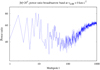 |
Fig. 24 Power ratio ℜ(l) for broad- and narrowband power distributions at vLSR = 0 km s−1. |
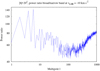 |
Fig. 25 Power ratio ℜ(l) for broad- and narrowband power distributions at vLSR = −10 km s−1. |
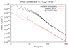 |
Fig. 26 EBHIS power spectra at intermediate velocities − 70 < vLSR < −30 km s−1 and fit for l > 8. |
8 Intermediate and high velocity clouds
Power spectra for thick velocity slices, discussed in the previous section, may be affected by emission from IVCs for large ΔvLSR. We have chosen the most prominent IVC emission in the velocity range − 70 < vLSR < −30 km s−1 and calculated the power distribution. The IVC emission is dominant on the northern hemisphere. To avoid any possible instrumental biases from a telescope mix we extracted EBHIS data, using the apodization schemes discussed in Appendix A.2.2. Our result is shown in Fig. 26. The all-sky data are obviously affected by spurious effects from differential Galactic rotation and do not represent genuine turbulent features. High latitude data show a straight power spectrum with an index γ = −2.620 ± 0.004, within possible systematical uncertainties Δγ ~ 0.05 in good agreement with γ = −2.68 ± 0.04 obtained by Martin et al. (2015), and − 2.60 ± 0.04≲γ≲ − 2.48 ± 0.06 by Blagrave et al. (2017). In comparison to a thick slice index of γ = −2.94 for the local H I, this is significantly flatter. No decomposition of the ICV emission in components from different H I phases is applied since such a separation for sources with unknown distances and beam smoothing effects appears to be ambiguous.
For the sake of completeness we also calculated power spectra for HVCs in the velocity range − 150 < vLSR < −100 km s−1. In this case as well we only used data from the northern hemisphere. The resulting power spectrum in Fig. 27 is useless in the all-sky case, but at high latitudes it is straight for 2 < l < 256 with γ = −2.0. This is even flatter than the index γ = −2.59 ± 0.07 observed by Martin et al. (2015) and γ = −2.85 ± 0.07 by Blagrave et al. (2017). Our power spectrum shows for multipoles l > 350 an S-shaped feature that cannot be explained by instrumental biases. For 350≲l≲700 there is a steepening to γ ~−3.2 with an abrupt flattening at high multipoles. This S-shaped feature comes from high latitude HVCs and is even more pronounced if we apodize data for |b| > 30°. An interpretation without further detailed investigations, which are beyond the scope of the current paper, is difficult. Perhaps this S-feature is caused by fragmentation and dissipation of HVCs on scales near 1°. The observed differences in spectral indices between our data and those of Martin et al. (2015) and Blagrave et al. (2017) may imply changes between different HVC complexes.
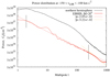 |
Fig. 27 EBHIS power spectra at intermediate velocities − 150 < vLSR < −100 km s−1 and fits for 2 < l < 256 and 350 < l < 700. |
9 Low multipoles – outer scale
It is broadly believed that the outer scale L, first mentioned in Sect. 3 and most likely defined by energy injection from old supernova remnant shock waves, must be close to L ~ 100 pc (Haverkorn et al. 2008). According to Chepurnov (1998), Cho & Lazarian (2002), and Mertsch & Sarkar (2013) the critical multipole lcrit for a broken power law dependson L and the scale height H of the turbulent medium, lcrit ~ 2πH∕L. The half width at half maximum scale height for the H I layer was determined to 115≲H≲140 pc (Dickey & Lockman 1990, Fig. 10 and Kalberla et al. 2007, Fig. 14), resulting in 7≲lcrit≲9. This is in good agreement with our finding that the power spectra tend, within the noise, to be shallow at l≲9. Strong multipole disparities are also mostly restricted to l≲9. (e.g., Figs. 1 and A.5).
Low multipoles l ≤ 8 were in all cases fit separately from the rest of the power distribution, using in this case constant weights. Figure 28 shows the derived velocity dependent power law indices. As an average over all fits for − 16 < vLSR < 16 km s−1 we determine γ = −0.66 ± 0.13 for the all-sky data and γ = −0.65 ± 0.09 for |b| > 20°.
Our estimate lcrit ~ 8 is consistent with Regis (2011) who determined lcrit = 10 ± 3 for the all-sky Galactic continuum emission from five radio maps and  at high latitudes. Our power law index γ = −0.65 ± 0.09 for l≲lcrit appears to be in conflict with the proposed value γ = −1. However, we need to consider that the index, derived for lcrit ~ 8, is probably influenced by the planar distribution of the Galactic H I. On large scales the column density distribution is dominated by cosecant latitude effects. Removing this effect leads to a change in the power distribution at low multipoles (see Sect. 3.3, and Fig. 4 in comparison to Fig. 1).
We use all-sky data, but our main conclusions are drawn from high latitudes, |b| > 20°. This region covers 67% of the sky with typical H I column densities below 1021 cm−2. We compare this region with that used by Planck Collaboration Int. XXX (2016). To study the angular power spectrum of polarized dust emission at intermediate and high Galactic latitudes, sky fractions between 30 and 80% were investigated by these authors to derive best-fit power law exponents. For multiploes l > 40 there are no significant changes in the best-fit power law exponents, in particular no changes for sky fractions of 70 and 80%. From these results, since gas and dust at high Galactic latitudes are well correlated with each other (Planck Collaboration XXIV 2011), we expect no significant cosecant latitude effects on our analysis of H I column densities for multipoles l≳10.
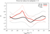 |
Fig. 28 Power law indices at low multipoles l < 9 for all-sky (black) and high latitudes (red). Thin lines indicate one-sigma upper and lower limits. The average γ = −0.66 is indicated by a dotted line. |
10 Summary and discussion
We use high resolution 21 cm line data from the HI4PI survey (HI4PI Collaboration 2016) to determine spatial power spectra for the H I in the local ISM. These panoramic observations enable us to derive spatial power spectra for multipoles 9≲l≲1023. The power distribution for multipoles l < 9 is consistentwith the assumption that turbulence has an outer scale close to 100 pc. Most of the observed multiphase H I power spectra are exceptionally straight in log–log presentation and can be fit well with constant spectral indices, γ ~ −2.94 for the local gas, γ ~−2.6 for IVCs, and γ ~−2 for HVCs. HVCs deviate from this rule and show some steepening at high multipoles. HI4PI power spectra for the emission from the complete Galactic plane can be contaminated seriously by confusion from differential Galactic rotation. H I data for several low latitude subfields within a range 98°≲l≲145° and − 20.4 < vLSR < 0.2 km s−1 were analyzed previously by Khalil et al. (2006). They derived γ = −2.95 ± 0.05, in good agreement with our result for the local gas at high latitudes.
The extraordinarily straight power distribution for the total H I at high latitudes with its well-defined broadband index of γ ~ −2.944 ± 0.005 (with possible systematic fluctuations on the order of Δγ ~ 0.05; see Appendix A.2.2) is in excellent agreement with dust spectral index γdust = −2.9 ± 0.1 determined by Miville-Deschênes et al. (2016) who also conclude from the straight power distribution that there is no sign of energy dissipation at the 0.01 pc scale. The power spectrum for the dust has to be interpreted as a spectrum of turbulent density fluctuations. Gas and dust are well mixed. The value γ ~ −2.94 for the total (phase independent) H I distribution must therefore be interpreted as characteristic of the total H I density distribution.
Phase transitions lead to modified distribution laws for individual phases (Saury et al. 2014). The observed filamentary CNM structures are well aligned with the magnetic field (Clark et al. 2014; Kalberla et al. 2016), resulting in asymmetries (Kalberla & Kerp 2016; Kalberla et al. 2017). The 3D space is no longer populated isotropically(Goldreich & Sridhar 1995). This probably implies a reduction in dimensionality, suggesting a flattening of the 3D power spectra for those parts of the H I that share the magnetic field orientation, the CNM, and the LNM.
We derive single-phase power spectra for CNM, LNM, and WNM from a Gaussian decomposition with characteristic linewidth regimes. These individual phases show power spectra that deviate significantlyfrom the multiphase power spectra. For all of the phases we get straight power spectra for 10 < l < 100 with indices γ ~ −2.5. In addition for l≳100 a strong increase in the power up to high multipoles is observed. The single-phase power spectra are, according to Eq. (4), highly correlated; the auto power relations for all phases must be considered together with all cross power terms between these phases. Thiscorrelation leads to counterintuitive consequences and contradictions if we try to describe the H I with several independentphases.
We find distinct correlations in velocity space. Coherence in the CNM is limited to a velocity spread of ~ 10 km s−1. Coherent features at high multipoles are identified as cold clumps with median Doppler temperatures of 223 K. Our analysis recovers structures that were previously described by Clark et al. (2014) and Kalberla et al. (2016). Trying to interpret these CNM structures as velocity caustics leads to contradictions. In particular, according to VCA the spectral index should steepen; however, we observe it to be undefined for velocity widths beyond 10 km s−1. These CNM features must be real entities in accordance with the findings of Clark et al. (2019). H I filaments on large scales are made up of aligned small-scale CNM structures. These CNM features show velocity fluctuations on larger scales, but these large-scale structures cannot be explained as being caused by velocity caustics.
Phase transition must be considered as local events with limitations in the cloud-cloud velocity dispersion for the resulting CNM clumps. For different bulk velocities we obtain coherence for different samples of CNM objects. The spectral coherence of the CNM is self-similar and statistically invariant under translation in velocity. The correlation between CNM and LNM implies that the LNM exists in connection with the CNM as a more extended phase, enveloping the CNM spatially but also covering a wider velocity spread of ~ 23 km s−1 as a transition to the more extended WNM. Self-similarity in velocity also applies to the LNM. Hence, associated with the hierarchical wave number scaling for phases with different linewidth domains we obtain a remarkable homogeneity in velocity space. Comparing power spectra for different hemispheres we find a high degree of isotropy.
The remarkable loss of correlation at large velocity lags is not in contradiction to the theoretical setup for the analysis of turbulent flows as considered by Kolmogorov (1941). The treatment of a turbulent flow needs to be restricted to a sufficiently small domain in four-dimensional space. Homogeneity and isotropy was explicitly defined by Kolmogorov as “local” only. These constraints, as described by Kolmogorov, correspond to the coherence conditions derived by us.
Restrictions in the velocity domain imply constraints for a velocity analysis, including the use of velocity centroids and explain discrepancies discovered previously by Kalberla et al. (2017, Appendix C). Our multiphase 3D spectral index γ = −2.94, derived with velocity constraints, is in conflict with steeper power law indices derived by Dickey et al. (2001) and Stanimirović & Lazarian (2001); however, these authors considered very different conditions. Dickey et al. (2001) got thick slice 3D spectral indices up to − 4.0 in the Galactic plane for velocities − 20 < vLSR < −80 km s−1, covering distances 1.5≲d≲13 kpc in the inner Galaxy. Stanimirović & Lazarian (2001) found a thick slice 3D spectral index of − 3.4 for the Small Magellanic Cloud, analyzing structures between 30 pc and 4 kpc perpendicular to the line of sight, integrating in velocity over ΔvLSR = 90 km s−1.
We use VCA (Lazarian & Pogosyan 2000) modified with restrictions in velocity space to disentangle density and velocity effects on observed power spectra. Taking velocity decorrelations into account, we derive single-phase estimates of Γρ ~ 0.5 for the spectral index of the density correlation function and Γv ~ 0.3 for the spectral index of the velocity correlation function for 10≲l≲100. For the total observed H I column density distribution we determine Γρ ~ 0.06 and Γv ~ 0.3 for all multipoles l≳9. The significance of the derived Γv ~ 0.3 must be questioned. A steepening of the power spectra as expected for velocity caustics can also be caused by phase transitions. For vLSR = 3 km s−1 we determine a CNM spectral index change δγ ~−0.4 from phase transitions, larger than the change δγ ~−0.14, indicated byVCA.
Spectral indices for single-channel power spectra are steepest at velocities close to zero km s−1 where CNM phase fractions are high and WNM phase fractions are low. We interpret this as an indication of local phase transitions. Phase transitions do not change the total column densities significantly, but decrease locally the line widths. Thus, thermal instabilities produce enhanced power in the line centers at the expense of the power in the wings of the line. At the same time phase transitions cause fragmentation, small-scale structure is generated, giving rise to enhanced power at high multipoles (l≳100). This process is necessarily accompanied by a decrease in power on scales that are characteristic of the regions that were affected by phase transitions and fragmentation. Power is reduced on intermediate scales and the power spectrum steepens for scales that are little affected by fragmentation (l≲100).
Recent high resolution simulations of thermal instabilities and collapsing cold clumps by Wareing et al. (2019) show that the density power spectrum can rapidly rise and steepen as the structures grow in the simulations. They find sheets and filaments on typical scales of 0.1–0.3 pc, consistent with high power for the CNM at large multipoles and also consistent with small-scale structures observed by Clark et al. (2014) and Kalberla et al. (2016). Previously Audit & Hennebelle (2005) and Federrath (2016) have derived a preferred scale of 0.1 pc from simulations. Our results appears to be in conflict with Saury et al. (2014) who find for subsonic turbulence that phase transitions lead to shallow power spectra with γ ~ −2.4. The discrepancy would be resolved if their analysis were sensitive to the single-phase CNM for which we observe γ ~ −2.37 at high latitudes.
Steep broadband 3D power law indices γ ~−3.6 that were previously considered to be characteristic for H I in emission deviate according to Hennebelle & Falgarone (2012, Fig 10) significantly from power law indices for molecular lines and other data. The single-phase power indices γ ~−2.5, derived by us, are in much better agreement with the other indices. This also applies to the comparison by Ghosh et al. (2017, Fig. 11). Cold filamentary H I structures were found to be correlated with Planck at 353 GHz polarized dust emission (Kalberla et al. 2016). Our broadband CNM power index of γ = −2.48 ± 0.04 fits well to the mean Planck intermediate latitude sky exponent of γ = −2.42 at 353 GHz for the EE and BB polarized dust power spectra at multipoles 40 < l < 370 (Planck Collaboration Int. XXX 2016). Ghosh et al. (2017) use in their dust model for the south Galactic pole region the CNM as a tracer of the dust polarization angle, and find for EE, BB, and TE modes spectral indices close to − 2.4, a value that they consider to be characteristic of the turbulent magnetic field as well. This is consistent with the results from Vansyngel et al. (2017) and more recently with Planck Collaboration XI (2019), who obtain an index of − 2.42 for the EE, − 2.54 for the BB, and − 2.49 for the TE mode. Adak et al. (2019) obtain for their dust model for the north Galactic pole region an index of − 2.4 ± 0.1 for EE, BB, and TE modes and the turbulent magnetic field, in excellent agreement with our value of γ = −2.48 for CNM and LNM at high latitudes.
Acknowledgements
We acknowledge the second anonymous referee for the constructive criticism. P.K. thanks Jürgen Kerp for the inspiring discussions and Bärbel Koribalski for the help with the LVHIS data. U.H. acknowledges the support from the Estonian Research Council grant IUT26-2, and from the European Regional Development Fund (TK133). This research has made use of NASA’s Astrophysics Data System. EBHIS is based on observations with the 100m telescope of the Max-Planck-Institut für Radioastronomie (MPIfR) at Effelsberg. The Parkes Radio Telescope is part of the Australia Telescope, which is funded by the Commonwealth of Australia for operation as a National Facility managed by CSIRO. Some of the results in this paper have been derived using the HEALPix package.
Appendix A Observations and data reduction
A.1 HI4PI 21-cm line survey data
We use HI4PI data (HI4PI Collaboration 2016), combining 21 cm line data from Effelsbeg-Bonn H I Survey (EBHIS), observed with the 100m Effelsberg radio telescope (Winkel et al. 2016a,b) and from the Galactic All Sky Survey (GASS), observed with the 64 m Parkes telescope (McClure-Griffiths et al. 2009; Kalberla et al. 2010; Kalberla & Haud 2015). EBHIS data from the first data release (Winkel et al. 2016b) and GASS data from the final data release (Kalberla & Haud 2015) were calibrated to a common intensity scale.
The multi-beam receivers scanned the sky, dumping spectra with short integration times (0.5 sec for EBHIS and 5 sec for GASS). Each of the individual dumps was corrected for stray radiation. The telescope data were gridded using Gaussian kernels of 5′.4 for EBHIS and 7′.5 for GASS, resulting in an effective FWHM beam size of 10.′8 for EBHIS, and 14.′5 for GASS. An nside = 1024 HEALPix database was chosen, appropriate for an angular resolution of Θpix = 3.′44 (Górski et al. 2005). This implies that our database is oversampled; neighboring positions are not independent from each other. Bandwidth limitations need to be taken into account, but a deconvolution (discussed below) for nside = 1024 is rather simple and well defined. For both telescopes a large number of dumps from the multi-beam receiver were averaged to generate profiles at the HEALPix grid positions, leading in each case to well-defined Gaussian beam shapes.
Combining data from different hemispheres we use a border line at δ = −2°. To avoid discontinuities caused by different beam sizes, we take a linear interpolation between the two surveys for − 4° < δ < 0°.
The 21 cm line surveys were observed with different spectrometers. For EBHIS the spectral resolution is δvLSR = 1.29 km s−1; for GASS it is δvLSR = 0.82 km s−1. The average noise for a single channel outside the H I line is 90 mK for the EBHIS and 55 mK for the GASS. We chose to interpolate the data to a common intermediate velocity grid with δvLSR = 1.03 km s−1, which is the velocity resolution of the LAB (Kalberla et al. 2005); the same database has been used previously (Kalberla et al. 2016). This interpolation causes for the EBHIS a slight increase in the average noise to 100 mK.
A.2 Instrumental effects
The observed intensities  can for individual telescope dumps be described by the convolution between the true distribution
  on the sky and the beam function
  of the telescope. In addition, we need to take into account the instrumental noise
  , which affects individual dumps:
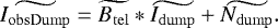 (A.1)
(A.1)
To get the intensity distribution on a HEALPix grid, the dump database is interpolated using a Gaussian weighting with an smoothing kernel  . This impliesan additional convolution and we obtain
 (A.2)
(A.2)
For convenience, we define here the smoothing function 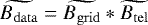 that was applied to the data.
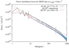 |
Fig. A.1 Raw single-channel spatial power distribution for observed H I column densities at vLSR =0 km s−1 without corrections for observational artifacts. To fit the spectral indices γ we only usedmultipoles 8 < l < 256. These limitsare indicated by the vertical lines. |
To calculate the power distribution we need to autocorrelate and perform a Fourier transform on Eq. (A.2), leading to
 (A.3)
(A.3)
with the cross power Pcross from  and
and 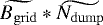
 (A.4)
(A.4)
or with Bdata = Bgrid Btel simplified to
 (A.5)
(A.5)
This result makes it necessary to correct the beam smoothing with different kernel functions for observed data and the noise term, and also to consider the question of whether the observations are affected by a cross term between noise and data. Smoothing and noise effects are discussed below in separate subsections. We also need to consider that EBHIS and GASS have different beam functions and different noise contributions. In data processing we have to process the two different hemispheres separately.
A.2.1 Apodization
If we want to analyze only a part of the sphere, in our case high latitudes with |b| > 20°, we need to take the window function into account that masks the observations. Since this window is applied to the brightness temperature distribution on the plane of the sky, it implies a smoothing to the observed power distribution Pobs(l). Sharp edgesof the window function may cause aliasing or power leakage between different multipoles l. To avoid such aliasing it is necessary to smooth the sharp edges of the window function by apodizing (Planck Collaboration XI 2016).
Figure A.1 shows the raw power spectrum for the observed column densities in a single channel at vLSR = 0 km s−1. We use this case here to demonstrate our data processing. The upper black profile presents the all-sky power spectrum; below we show two versions of the power spectrum at high latitudes, |b| > 20°. The cyan spectrum in Fig. A.1 shows Pobs(l) after setting in ANAFAST the parameter theta_cut_deg (or gal_cut in healpy) to 20°. We observe strong aliasing caused by an observational window with sharp cutoff at 20°; an apodization is needed to overcome spurious effects.
Similar to Kalberla & Kerp (2016) we use a cosine taper (a Tukey window; Harris 1978) for apodization in latitude b. After a few tests we chose a taper width with a half-period of 15°, weighting smoothly from one at |b| = 20° to zero at |b| = 5°. The resulting power spectrum is shown in Fig. A.1 in red, overplotted on the unapodized case. Testing a narrower cosine taper, for example with a half-period of 10°, we found still significant unwanted aliasing effects. A broader cosine taper for |b| = 20° is also not appropriate since it leads to a leakage of Galactic plane emission from |b| < 5°. Any apodization window leads to unwanted side effects (Harris 1978), but this apodization-ringing decreases as the width of the window increases. Remaining problems (Fig. A.1, red curve) are acceptable for our analysis with minor errors, as demonstrated in Fig. 4. The optimal width of the Tukey window that we applied is slightly larger then the σ = 5° Gaussian taper used for the apodization map generated by the cosmological parameters team (Planck Collaboration XI 2016).
A.2.2 Beam smoothing
Observed brightness temperatures are smoothed by the beam function. In addition we need to take into account that for each cell of the HEALPix grid the data are interpolated. The resulting effective beam, has a FWHM beam width of 10′.8 for EBHIS (Winkel et al. 2016a). For the GASS we needed to redetermine the FWHM beamwidth since we use the third data release (Kalberla & Haud 2015) with some improvements over the second release Kalberla et al. (2010). We searched the Local Volume H I Survey (Koribalski et al. 2018) for appropriate point-like narrowband H I sources and used the barred Magellanic irregular galaxy IC 4662 (van Eymeren et al. 2010) which has at vLSR = 324 km s−1 a bright compact 2′ core. In addition, the beam width was determined from the ultra-compact high velocity cloud HVC289+33+251 (Putman et al. 2002; Brüns & Westmeier 2004) with a FWHM size of 4′.4. Fitting the sizes of these sources we derive a FWHM beamwidth of 14′.5 ± 0.′2 which compares well with the beamwidth of 14.′4 determined by Calabretta et al. (2014). This 14.′5 beam is a considerable improvement over the second GASS data release with an effective beam width of 15′.9 in the presence of residual instrumental errors.
We consider once more a single channel at vLSR = 0 km s−1 (see Fig. A.1). The upper all-sky power spectrum (black) and the lower one (red and apodized for |b| = 20°), both suffer for l≳256 from beam smoothing. We observe a steepening of the spectral index at high multipoles, which without beam correction may be mistaken as a real effect, for example as steepening caused by a change in slice thickness (Lazarian & Pogosyan 2000). For the raw data shown in Fig. A.1 essentially only a limited range, l < 256, as indicated by a vertical bar, can be used to fit the spectral index γ. It is essential to correct for beam smoothing if we want to avoid instrumental biases.
To evaluate beam smoothing effects we separate the emission observed in different hemispheres. We use a 15° cosine apodization scheme, extracting data for EBHIS at declinations δ > 13° and for GASS at δ < −17°. Figure A.2 (top) shows the correlation coefficients for EBHIS (left panel) and GASS (right panel). The black lines show significant differences in beam smoothing caused by different beam widths. We correct in both cases the observed power spectra by applying corrections based on the effective FWHM beam widths, 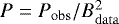 according to the first term in Eq. (A.4). Bdata(l) is telescope dependent and includes beam smoothing and smoothing caused by gridding. The power spectra, including their fits for 8 < l < 1023 are shown in magenta. A comparison between observed and beam corrected power spectra shows that differences can be seen for l≳256, corresponding to angular scales of θ ~ 180°∕l ~ 42′ or about three to four FWHM beam widths. In the case of noisy data, the beam smoothing effects may not be recognizableuntil scales corresponding to one beam width. This does not imply that beam corrections are not necessary.
Merging disjunct data from EBHIS and GASS makes it necessary to correct at once for beam effects from both telescopes. For an isotropic power distribution this is fortunately very simple; at any multipole l the power from the two telescopes is summed; we can correct for beam effects by using a weighted average beam function, taking the borderline at δ= −2° into account. The lower left plot in Fig. A.2 can serve as a proof. Finally, we compare the corrected power spectra in the lower panel to the right side of Fig. A.2. The spectra from EBHIS and GASS agree well; the sum of the two power distributions is shown in red. This sum contains apodized regions; therefore, we also plot the unapodized all-sky power spectrum. This comparison shows a nearly isotropic power distribution between thetwo disjunct hemispheres, but there are systematic changes in the spectral index. We obtain − 2.717 > γ > −2.810 with an average of γ= −2.768, hence a deviation of up to Δγ ~ 0.05 from the all-sky index. This is more than a factor of ten larger than the formal one-sigma uncertainty for an individual fit in the range for 8 < l < 1023. The change of the spectral index reflects changes in the source distribution and is predominantly caused by differences at low multipoles.
A.2.3 System noise
It has been demonstrated by Kalberla & Kerp (2016) that a beam correction according to Eq. (2) leads in general to an amplification of instrumental uncertainties at high multipoles. However, for l≲1023 we do not observe an obvious increase in Fig. A.2.
To check whether our analysis might be degraded by unrecognized system noise, we generate all-sky random noise maps as expected from the system performance of the two telescopes. The system noise Tsys contains several contributions. Most important is the thermal noise from the receiver system and the elevation dependent ground radiation including spill-over. Next there is the position dependent continuum sky background. All these components are variable, but we use here an average thermal contribution Tsys = 30 K. The line signal TB (vLSR) adds to the frequency independent part and thenoise contribution TNoise(vLSR) to the H I data can then be approximated as (Haud 2000)
![Mathematical equation: \begin{equation*} T_{ \mathrm{Noise}} (v_{\mathrm{LSR}}) = \sigma_{ \mathrm{av}} [T_{ \mathrm{sys}} + T_{ \mathrm{B}} (v_{\mathrm{LSR}}) ] / T_{\mathrm{sys}},\end{equation*}](/articles/aa/full_html/2019/07/aa34533-18/aa34533-18-eq30.png) (A.6)
(A.6)
where σav is the average noise level, determined at velocities without H I line emission.
Figure A.3 shows a noise power spectrum for such a simulation of the observational conditions for TB (vLSR) ~ 0 K after deconvolution for the telescope beams at velocities without H I line emission. We overlay this estimate with the power distribution  derived for a single channel observed at the velocity vLSR = 400 km s−1, without significant H I emission. The cross term 2Pcross in Eq. (A.5) is therefore zero. Comparing the observed power distribution with the expected distribution, we find agreement for l≳300 but significant deviations at low multipoles, typically for single-dish telescopes (e.g., Martin et al. 2015, Figs. 6 and 9). Assuming a constant σav is only a poor approximation of the observed noise power (see Kalberla et al. 2010, Fig. 9 and Winkel et al. 2016a, Fig. 14). The observational setup causes unavoidable deviations from a random noise, in particular blocky structures, which in turn lead to enhanced power at low multipoles. To improve the noise template we need to replace the averages σav, Tsys, with position dependent values in Eq. (A.6). For each of the telescope dumps and HEALPix positions the rms fluctuations in the baseline regions are known and can also be used. This more sophisticated scheme was used to control the Gaussian decomposition (Haud 2000; Kalberla & Haud 2015, 2018), but here we found that it was not necessary to elaborate Eq. (A.6) further.
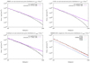 |
Fig. A.2 Power distributions at vLSR = 0 km s−1, comparing single-channel H I column densities for EBHIS (top left) and GASS (top right) with the all-sky combination of both surveys (bottom left). The black lines indicate power spectra derived from raw observations, the magenta lines are beam corrected power spectra with fits. On the lower panel to the right we compare the beam corrected power spectra. |
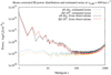 |
Fig. A.3 Spatial power distribution |


We apply our simple noise model to the single channel H I data at vLSR = 0 km s−1 shown in Fig. A.1. In comparison to Fig. A.3 the line emission term TB (vLSR) in Eq. (A.6) is significant, leading to an enhancement of the noise power. In addition, TB (vLSR)≠0 K implies that the noise depends on the intensity distribution on the sky, and  from Eq. (A.5) needs to be taken into account. In Fig. A.4 we compare the estimated noise contribution and the cross power with the beam corrected power spectrum. The noise contribution
  is critical at high multipoles, but due to the good S/N of the HI4PI data this noise power is, in the worst case, at l = 1023 more than an order of magnitude below the H I signal
  . The noise cross power
  scales with
  , but is aboutthree orders of magnitude below the relevant H I power signal. Altogether, this is a very comfortable result, reflecting that the HI4PI survey has a good S/N.
For H I in the profile wings considered by us, for example at |vLSR| = 16 km s−1, the noise power is still more than a factor of five below the line signal. Our noise template according to Eq. (A.6) can be applied to different velocity widths and we obtain in this case a simple scaling relation. Averaging n channels decreases the noise power contribution by a factor of n, but at the same time the H I power increases. For a total bandwidth of ΔvLSR = 16 km s−1 the expected noise contribution is, in the worst case, more than four orders of magnitude below the observed signal. Noise limitations, including other remaining instrumental uncertainties, are not important for HI4PI data as used by us. For most of our analysis we can safely disregard the noise term Noise(l) in Eq. (2).
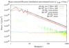 |
Fig. A.4 Beam corrected power distribution |

A.3 Intrinsic uncertainties in parameter fitting
We learn from the noise simulations that the scatter of Cl(l) is for white noise increasing at low multipoles l (see Fig. A.3). This is a general property of angular power spectra with finite counts (Campbell 2015, Eq. (5)) and we expect for the estimator Ĉl
![Mathematical equation: \begin{equation*} \textrm{Var}({\hat{C}_l})/[ N_l + C_l ]^2 = 2/(2l+1).\end{equation*}](/articles/aa/full_html/2019/07/aa34533-18/aa34533-18-eq37.png) (A.7)
(A.7)
Var (Ĉl) is usually called cosmic variance. In Fig. A.5 we show an example of single-channel data at vLSR = 0 km s−1. When fittingpower spectra we take dispersions  into account. Fitting is done iteratively with constant weights for an initial estimate of Ĉl, next using derived weights to improve the error estimate for the final fit with χ2 ∕NDOF≲1. We quote for the power spectral indices formal one-sigma uncertainties from the fit. Systematic fluctuations between different hemispheres amount to Δγ ~ 0.05 (Appendix A.2.2) and may be more characteristic for the overall uncertainties. Differences between the initial estimate and the final fit are typically less than or about one sigma. In general we find a large scatter for Cl at low multipoles l≲8 with tendencies for even-odd oscillations. Large-scale symmetries of the Galactic H I emission cause an enhanced disparity between even and odd modes (Mertsch & Sarkar 2013). These disparities disappear mostly for higher multipoles, and therefore we exclude in general multipoles l ≤ 8 when fittingspectral indices for the H I distribution.
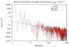 |
Fig. A.5 Intrinsic uncertainties |

References
- Adak, D., Ghosh, T., Boulanger, F., et al. 2019, ArXiv e-prints [arXiv:1906.07445] [Google Scholar]
- Audit, E., & Hennebelle, P. 2005, A& A, 433, 1 [CrossRef] [EDP Sciences] [Google Scholar]
- Blagrave, K., Martin, P. G., Joncas, G., et al. 2017, ApJ, 834, 126 [NASA ADS] [CrossRef] [Google Scholar]
- Burkhart, B., Stanimirović, S., Lazarian, A., & Kowal, G. 2010, ApJ, 708, 1204 [NASA ADS] [CrossRef] [Google Scholar]
- Burton, W. B. 1972, A&A, 19, 51 [NASA ADS] [Google Scholar]
- Brüns, C., & Westmeier, T. 2004, A&A, 426, L9 [NASA ADS] [CrossRef] [EDP Sciences] [Google Scholar]
- Calabretta, M. R., Staveley-Smith, L., & Barnes, D. G. 2014, PASA, 31, e007 [Google Scholar]
- Campbell, S. S. 2015, MNRAS, 448, 2854 [NASA ADS] [CrossRef] [Google Scholar]
- Chepurnov, A. V. 1998, Astron. Astrophys. Trans., 17, 281 [Google Scholar]
- Chepurnov, A., Lazarian, A., Stanimirović, S., Heiles, C., & Peek, J. E. G. 2010, ApJ, 714, 1398 [NASA ADS] [CrossRef] [Google Scholar]
- Cho, J., & Lazarian, A. 2002, ApJ, 575, L63 [NASA ADS] [CrossRef] [Google Scholar]
- Choudhuri, S., & Roy, N. 2019, MNRAS, 483, 3437 [NASA ADS] [CrossRef] [Google Scholar]
- Clark, S. E., Peek, J. E. G., & Putman, M. E. 2014, ApJ, 789, 82 [NASA ADS] [CrossRef] [Google Scholar]
- Clark, S. E., Peek, J. E. G., & Miville-Deschênes, M.-A. 2019, ApJ, 874, 171 [NASA ADS] [CrossRef] [Google Scholar]
- Crovisier, J., & Dickey, J. M. 1983, A&A, 122, 282 [NASA ADS] [Google Scholar]
- Dickey, J. M., & Lockman, F. J. 1990, ARA&A, 28, 215 [NASA ADS] [CrossRef] [MathSciNet] [Google Scholar]
- Dickey, J. M., McClure-Griffiths, N. M., Stanimirović, S., Gaensler, B. M., & Green, A. J. 2001, ApJ, 561, 264 [NASA ADS] [CrossRef] [MathSciNet] [Google Scholar]
- Dedes, L., & Kalberla, P. M. W. 2012, EAS Pub. Ser., 56, 209 [CrossRef] [Google Scholar]
- Deshpande, A. A., Dwarakanath, K. S., & Goss, W. M. 2000, ApJ, 543, 227 [NASA ADS] [CrossRef] [Google Scholar]
- Elmegreen, B. G., & Scalo, J. 2004, ARA&A, 42, 211 [NASA ADS] [CrossRef] [Google Scholar]
- Elmegreen, B. G., Kim, S., & Staveley-Smith, L. 2001, ApJ, 548, 749 [NASA ADS] [CrossRef] [Google Scholar]
- Federrath, C. 2016, MNRAS, 457, 375 [NASA ADS] [CrossRef] [Google Scholar]
- Ghosh, T., Boulanger, F., Martin, P. G., et al. 2017, A&A, 601, A71 [NASA ADS] [CrossRef] [EDP Sciences] [Google Scholar]
- Goldreich, P., & Sridhar, S. 1995, ApJ, 438, 763 [NASA ADS] [CrossRef] [Google Scholar]
- Górski, K. M., Hivon, E., Banday, A. J., et al. 2005, ApJ, 622, 759 [NASA ADS] [CrossRef] [Google Scholar]
- Green, D. A. 1993, MNRAS, 262, 327 [NASA ADS] [CrossRef] [Google Scholar]
- Haverkorn, M., Brown, J. C., Gaensler, B. M., & McClure-Griffiths, N. M. 2008, ApJ, 680, 362 [NASA ADS] [CrossRef] [Google Scholar]
- Harris, F. J. 1978, IEEE Proc., 66, 51 [Google Scholar]
- Haud, U. 2000, A&A, 364, 83 [NASA ADS] [Google Scholar]
- Haud, U. 2008, A&A, 483, 461 [NASA ADS] [CrossRef] [EDP Sciences] [Google Scholar]
- Heiles, C., & Troland, T. H. 2003, ApJ, 586, 1067 [NASA ADS] [CrossRef] [Google Scholar]
- Heiles, C., & Crutcher, R. 2005, Cosmic Magnetic Fields (Berlin: Springer Science & Business Media), 664, 137 [Google Scholar]
- Heiles, C., & Troland, T. H. 2005, ApJ, 624, 773 [NASA ADS] [CrossRef] [Google Scholar]
- Hennebelle, P., & Falgarone, E. 2012, A&ARv, 20, 55 [NASA ADS] [CrossRef] [Google Scholar]
- HI4PI Collaboration (Ben Bekhti, et al.) 2016, A&A, 594, A116 [NASA ADS] [CrossRef] [EDP Sciences] [Google Scholar]
- Jelić, V., Prelogović, D., Haverkorn, M., Remeijn, J., & Klindžić, D. 2018, A&A, 615, L3 [NASA ADS] [CrossRef] [EDP Sciences] [Google Scholar]
- Mebold, U. 1972, A&A, 19, 13 [NASA ADS] [Google Scholar]
- Kalberla, P. M. W., & Mebold, U. 1983, Mitt. Astron. Ges. Hamburg, 58, 101 [NASA ADS] [Google Scholar]
- Kalberla, P. M. W., & Haud, U. 2015, A&A, 578, A78 [NASA ADS] [CrossRef] [EDP Sciences] [Google Scholar]
- Kalberla, P. M. W., & Kerp, J. 2016, A&A, 595, A37 [NASA ADS] [CrossRef] [EDP Sciences] [Google Scholar]
- Kalberla, P. M. W., & Haud, U. 2018, A&A, 619, A58 [NASA ADS] [CrossRef] [EDP Sciences] [Google Scholar]
- Kalberla, P. M. W., Burton, W. B., Hartmann, D., et al. 2005, A&A, 440, 775 [NASA ADS] [CrossRef] [EDP Sciences] [Google Scholar]
- Kalberla, P. M. W., Dedes, L., Kerp, J., & Haud, U. 2007, A&A, 469, 511 [NASA ADS] [CrossRef] [EDP Sciences] [Google Scholar]
- Kalberla, P. M. W., McClure-Griffiths, N. M., Pisano, D. J., et al. 2010, A&A, 521, A17 [NASA ADS] [CrossRef] [EDP Sciences] [Google Scholar]
- Kalberla, P. M. W., Kerp, J., Haud, U., et al. 2016, ApJ, 821, 117 [NASA ADS] [CrossRef] [Google Scholar]
- Kalberla, P. M. W., Kerp, J., Haud, U., & Haverkorn, M. 2017, A&A, 607, A15 [NASA ADS] [CrossRef] [EDP Sciences] [Google Scholar]
- Khalil, A., Joncas, G., Nekka, F., Kestener, P., & Arneodo, A. 2006, ApJS, 165, 512 [NASA ADS] [CrossRef] [Google Scholar]
- Kolmogorov, A. N. 1941, Akad. Nauk SSSR Dokl., 30, 301 (translation by V. Levin 1991, Proc. R. Soc. Lond. A, 434, 9 [Google Scholar]
- Kolmogorov, A. N. 1962, J. Fluid Mech., 13, 82 [NASA ADS] [CrossRef] [Google Scholar]
- Koribalski, B. S., Wang, J., Kamphuis, P., et al. 2018, MNRAS, 478, 1611 [NASA ADS] [CrossRef] [Google Scholar]
- Lazarian, A. 2009, Space Sci. Rev., 143, 357 [NASA ADS] [CrossRef] [Google Scholar]
- Lazarian, A., & Pogosyan, D. 2000, ApJ, 537, 720 [NASA ADS] [CrossRef] [Google Scholar]
- Lazarian, A., & Pogosyan, D. 2006, ApJ, 652, 1348 [NASA ADS] [CrossRef] [Google Scholar]
- Lazarian, A., & Yuen, K. H. 2018, ApJ, 853, 96 [NASA ADS] [CrossRef] [Google Scholar]
- Lee, M.-Y., Stanimirović, S., Murray, C. E., Heiles, C., & Miller, J. 2015, ApJ, 809, 56 [NASA ADS] [CrossRef] [Google Scholar]
- Martin, P. G., Blagrave, K. P. M., Lockman, F. J., et al. 2015, ApJ, 809, 153 [NASA ADS] [CrossRef] [Google Scholar]
- McClure-Griffiths, N. M., Pisano, D. J., Calabretta, M. R., et al. 2009, ApJS, 181, 398 [NASA ADS] [CrossRef] [Google Scholar]
- McKee, C. F., & Ostriker, J. P. 1977, ApJ, 218, 148 [NASA ADS] [CrossRef] [Google Scholar]
- Mertsch, P., & Sarkar, S. 2013, JCAP, 6, 041 [NASA ADS] [CrossRef] [Google Scholar]
- Miville-Deschênes, M.-A., & Martin, P. G. 2007, A&A, 469, 189 [NASA ADS] [CrossRef] [EDP Sciences] [Google Scholar]
- Miville-Deschênes, M.-A., Joncas, G., Falgarone, E., & Boulanger, F. 2003, A&A, 411, 109 [NASA ADS] [CrossRef] [EDP Sciences] [Google Scholar]
- Miville-Deschênes, M.-A., Duc, P.-A., Marleau, F., et al. 2016, A&A, 593, A4 [NASA ADS] [CrossRef] [EDP Sciences] [Google Scholar]
- Murray, C. E., Stanimirović, S., Goss, W. M., et al. 2018a, ApJS, 238, 14 [NASA ADS] [CrossRef] [Google Scholar]
- Murray, C. E., Peek, J. E. G., Lee, M.-Y., & Stanimirović, S. 2018b, ApJ, 862, 131 [NASA ADS] [CrossRef] [Google Scholar]
- Pingel, N. M., Stanimirović, S., Peek, J. E. G., et al. 2013, ApJ, 779, 36 [NASA ADS] [CrossRef] [Google Scholar]
- Pingel, N. M., Lee, M.-Y., Burkhart, B., & Stanimirović, S. 2018, ApJ, 856, 136 [NASA ADS] [CrossRef] [Google Scholar]
- Planck Collaboration XXIV. 2011, A&A, 536, A24 [Google Scholar]
- Planck Collaboration XI. 2016, A&A, 594, A11 [NASA ADS] [CrossRef] [EDP Sciences] [Google Scholar]
- Planck Collaboration Int. XXX. 2016, A&A, 586, A133 [NASA ADS] [CrossRef] [EDP Sciences] [Google Scholar]
- Planck Collaboration XI. 2019, A&A, in press, DOI: 10.1051/0004-6361/201832618 [Google Scholar]
- Putman, M. E., de Heij, V., Staveley-Smith, L., et al. 2002, AJ, 123, 873 [NASA ADS] [CrossRef] [Google Scholar]
- Regis, M. 2011, Astropart. Phys., 35, 170 [NASA ADS] [CrossRef] [Google Scholar]
- Roy, N., Chengalur, J. N., Dutta, P., & Bharadwaj, S. 2010, MNRAS, 404, L45 [NASA ADS] [CrossRef] [Google Scholar]
- Roy, N., Minter, A. H., Goss, W. M., Brogan, C. L., & Lazio, T. J. W. 2012, ApJ, 749, 144 [NASA ADS] [CrossRef] [Google Scholar]
- Saury, E., Miville-Deschênes, M.-A., Hennebelle, P., Audit, E., & Schmidt, W. 2014, A&A, 567, A16 [NASA ADS] [CrossRef] [EDP Sciences] [Google Scholar]
- Scalo, J., & Elmegreen, B. G. 2004, ARA&A, 42, 275 [NASA ADS] [CrossRef] [Google Scholar]
- Schneider, N., Bontemps, S., Simon, R., et al. 2011, A&A, 529, A1 [NASA ADS] [CrossRef] [EDP Sciences] [Google Scholar]
- Stanimirović,S., & Lazarian, A. 2001, ApJ, 551, L53 [NASA ADS] [CrossRef] [Google Scholar]
- Stanimirovic, S., Staveley-Smith, L., Dickey, J. M., Sault, R. J., & Snowden, S. L. 1999, MNRAS, 302, 417 [NASA ADS] [CrossRef] [Google Scholar]
- Sun, K., Kramer, C., Ossenkopf, V., et al. 2006, A&A, 451, 539 [NASA ADS] [CrossRef] [EDP Sciences] [Google Scholar]
- van Eymeren, J., Koribalski, B. S., López-Sánchez, Á. R., Dettmar, R.-J., & Bomans, D. J. 2010, MNRAS, 407, 113 [NASA ADS] [CrossRef] [Google Scholar]
- van Woerden, H., Wakker, B. P., Schwarz, U. J., & de Boer, K. S. 2004, High Velocity Clouds (Berlin: Springer Science & Business Media), 312 [Google Scholar]
- Vansyngel, F., Boulanger, F., Ghosh, T., et al. 2017, A&A, 603, A62 [NASA ADS] [CrossRef] [EDP Sciences] [Google Scholar]
- Vazquez-Semadeni, E. 1994, ApJ, 423, 681 [NASA ADS] [CrossRef] [Google Scholar]
- Vázquez-Semadeni, E. 2012, EAS Pub. Ser., 56, 39 [Google Scholar]
- Wakker, B. P., & van Woerden, H. 1997, ARA&A, 35, 217 [NASA ADS] [CrossRef] [Google Scholar]
- Wareing, C. J., Falle, S. A. E. G., & Pittard, J. M. 2019, MNRAS, 485, 4686 [NASA ADS] [CrossRef] [Google Scholar]
- Winkel, B., Kerp, J., Flöer, L., et al. 2016a, A&A, 585, A41 [NASA ADS] [CrossRef] [EDP Sciences] [Google Scholar]
- Winkel, B., Lenz, D., & Flöer, L. 2016b, A&A, 591, A12 [NASA ADS] [CrossRef] [EDP Sciences] [Google Scholar]
- Wolfire, M. G., McKee, C. F., Hollenbach, D., & Tielens, A. G. G. M. 2003, ApJ, 587, 278 [NASA ADS] [CrossRef] [Google Scholar]
- Yuen, K. H., Hu, Y., Lazarian, A., & Pogosyan, D. 2019, ArXiv e-prints [arXiv:1904.03173] [Google Scholar]
Interview of Hendrik van de Hulst on 6 September 1978 at Leiden by W. T. Sullivan III, https://www.nrao.edu/archives/Sullivan/sullivan_interviewee_vandehulst.shtml
For calculations of the CMB, power spectra of the kind l(l + 1)Cl are usually considered. Here we do not follow this convention, but use simply Cl. This way the power exponent γ increases by two.
In Eq. (51) of Lazarian & Pogosyan (2000) the cross term between CNM and WNM in the case of a two-component medium is defined without the factor two in our Eq. (4).
For a turbulent medium the characteristic PDFs are log-normal (Vazquez-Semadeni 1994) as a result of the central limit theorem applied to self-similar random multiplicative perturbations. The geometric mean of a log-normal distribution is equal to its median.
All Figures
|
Fig. 1 Power distributions for different H I phases at vLSR = 0 km s−1. Top left: WNM; top right: LNM; bottom left: CNM; andbottom right: sum of all phases with uncertainties from the Gaussian decomposition (cyan and orange). Black lines show all-sky data, red lines are for |b| > 20°. Spectral indices γ for CNM, LNM, and CNM are derived at 10 < l < 100 and for the sum of all phases at l > 8 as indicated by the vertical lines. |
| In the text | |
|
Fig. 2 Cross power spectra between WNM and CNM (PWxC), WNM and LNM (PWxL), and LNM and CNM (PLxC) at vLSR = 0 km s−1. |
| In the text | |
|
Fig. 3 Cross power spectra between WNM and CNM (PWxC), WNM and LNM (PWxL), and LNM and CNM (PLxC) at vLSR = 0 km s−1. |
| In the text | |
|
Fig. 4 Power distributions for phase fractions in different H I phases at vLSR = 0 km s−1. Top left: WNM; top right: LNM; bottom left: CNM. Black lines show all-sky data, red lines are for |b| > 20°. Spectral indices are derived at 10 < l < 100 as indicated by the vertical lines. Bottom right: uncertainties from the Gaussian decomposition (black) and ringing caused by apodization (red). |
| In the text | |
|
Fig. 5 Velocity distribution of average H I phase fractions for CNM, LNM, and WNM using unpublished data from Kalberla & Haud (2018). |
| In the text | |
|
Fig. 6 All-sky velocity dependences of spectral indices for H I phase fractions. The thin lines represent the scatter for one-sigma uncertainties. |
| In the text | |
|
Fig. 7 High latitude velocity dependences of spectral indices for H I phase fractions. The thin lines represent the scatter for one-sigma uncertainties. |
| In the text | |
|
Fig. 8 All-sky velocity dependences of spectral indices for individual phases, and the total H I distribution (black). The thin lines represent the scatter for one-sigma uncertainties when the total H I distribution (black) uncertainties are within the thickness of the line. |
| In the text | |
|
Fig. 9 High latitude velocity dependences of spectral indices for individual phases, and the total H I distribution (red). The thin lines represent the scatter for one-sigma uncertainties when the total H I distribution (red) uncertainties are within the thickness of the line. |
| In the text | |
|
Fig. 10 Power ratio ℜ(l) according to Eq. (7). The ON velocity is vLSR = 3 km s−1; OFF is calculated as the average of single-channel slices at vLSR = −3 and 7 km s−1. The dotted line indicates ℜ(l) = 1. |
| In the text | |
|
Fig. 11 Power ratio 𝔈(l) according to Eq. (8). The ON velocity is vLSR = 3 km s−1; OFF is calculated as the average of single-channel slices at vLSR = −3 and 7 km s−1. The spectral index for the total HI is calculated for l > 10; in the case ofthe CNM for 10 < l < 100, the horizontal lines indicate these limits. |
| In the text | |
|
Fig. 12 All-sky dependences of spectral indices for H I phase fractions and velocity channel width. The thin lines represent the scatter for one-sigma uncertainties. |
| In the text | |
|
Fig. 13 Dependences of spectral indices for H I phase fractions and velocity channel width at |b| > 20°. The thin lines represent the scatter for one-sigma uncertainties. |
| In the text | |
|
Fig. 14 All-sky dependences of spectral indices for observed H I column densities as a function of the velocity channel width. The thin lines represent the scatter for one-sigma uncertainties. |
| In the text | |
|
Fig. 15 Cross-correlations at latitudes |b| > 20° between two channels at vLSR = −5 and vLSR = +5 for the WNM, LNM, and CNM. |
| In the text | |
|
Fig. 16 Spectral coherence for velocity slices at vLSR = −5 km s−1 and vLSR =+5 km s−1 for the total H I, WNM, LNM, and CNM. |
| In the text | |
|
Fig. 17 Spectral coherence for velocity slices at vLSR = −2 km s−1 and vLSR =2 km s−1 for the WNM, LNM, and CNM. |
| In the text | |
|
Fig. 18 Spectral coherence for velocity slices at vLSR = 6 km s−1 and vLSR =10 km s−1 for the WNM, LNM, and CNM. |
| In the text | |
|
Fig. 19 Spectral coherence Sl(v1, v2) for WNM and LNM velocity slices. The labels indicate the velocities v1 and v2 and the phases, WNM (W) or LNM (L). |
| In the text | |
|
Fig. 20 Dependences of the spectral coherence Sl(v1, v2) on the lag Δv = v2 − v1 for the CNMand LNM at |b| > 20°. Averages for multipoles l < 1000 are given (points) in comparison with Gaussian distributions with FWHM widths of 3.2 and 10 km s−1 (lines). |
| In the text | |
|
Fig. 21 Single-channel spatial coherences Pl at vLSR= 0 km s−1 for CNM, LNM, and WNM. |
| In the text | |
|
Fig. 22 All-sky cross-correlations between vLSR = −13 and vLSR = +13 for the totalH I, WNM, LNM, and CNM. |
| In the text | |
|
Fig. 23 Power distributions for different H I phases at − 8 < vLSR < 8 km s−1. Top left: WNM; top right: LNM; bottom left: CNM; and bottom right: sum of all phases with uncertainties from the Gaussian decomposition (cyan and orange). Black lines show all-sky data; red lines are for |b| > 20°. Spectral indices γ for CNM, LNM, and CNM are derived at 10 < l < 100 for the sum of all phases at l > 8, as indicated by the vertical lines. |
| In the text | |
|
Fig. 24 Power ratio ℜ(l) for broad- and narrowband power distributions at vLSR = 0 km s−1. |
| In the text | |
|
Fig. 25 Power ratio ℜ(l) for broad- and narrowband power distributions at vLSR = −10 km s−1. |
| In the text | |
|
Fig. 26 EBHIS power spectra at intermediate velocities − 70 < vLSR < −30 km s−1 and fit for l > 8. |
| In the text | |
|
Fig. 27 EBHIS power spectra at intermediate velocities − 150 < vLSR < −100 km s−1 and fits for 2 < l < 256 and 350 < l < 700. |
| In the text | |
|
Fig. 28 Power law indices at low multipoles l < 9 for all-sky (black) and high latitudes (red). Thin lines indicate one-sigma upper and lower limits. The average γ = −0.66 is indicated by a dotted line. |
| In the text | |
|
Fig. A.1 Raw single-channel spatial power distribution for observed H I column densities at vLSR =0 km s−1 without corrections for observational artifacts. To fit the spectral indices γ we only usedmultipoles 8 < l < 256. These limitsare indicated by the vertical lines. |
| In the text | |
|
Fig. A.2 Power distributions at vLSR = 0 km s−1, comparing single-channel H I column densities for EBHIS (top left) and GASS (top right) with the all-sky combination of both surveys (bottom left). The black lines indicate power spectra derived from raw observations, the magenta lines are beam corrected power spectra with fits. On the lower panel to the right we compare the beam corrected power spectra. |
| In the text | |
|
Fig. A.3 Spatial power distribution |
| In the text | |
|
Fig. A.4 Beam corrected power distribution |
| In the text | |
|
Fig. A.5 Intrinsic uncertainties |
| In the text | |
Current usage metrics show cumulative count of Article Views (full-text article views including HTML views, PDF and ePub downloads, according to the available data) and Abstracts Views on Vision4Press platform.
Data correspond to usage on the plateform after 2015. The current usage metrics is available 48-96 hours after online publication and is updated daily on week days.
Initial download of the metrics may take a while.