| Issue |
A&A
Volume 627, July 2019
|
|
|---|---|---|
| Article Number | A162 | |
| Number of page(s) | 12 | |
| Section | Interstellar and circumstellar matter | |
| DOI | https://doi.org/10.1051/0004-6361/201834184 | |
| Published online | 17 July 2019 | |
A particular carbon-chain-producing region: L1489 starless core★
1
Department of Astronomy, Peking University,
100871
Beijing,
PR China
e-mail: ywu@pku.edu.cn
2
School of Astronomy and Space Sciences, University of Science and Technology of China,
96 Jinzhai Road,
Hefei
230026, PR China
3
Purple Mountain Observatory and Key Laboratory of Radio Astronomy, Chinese Academy of Sciences,
8 Yuanhua Road,
Nanjing
210034, PR China
4
Shanghai Astronomical Observatory, Chinese Academy of Sciences,
Shanghai
200030,
PR China
5
Center for Astrophysics, GuangZhou University,
Guangzhou
510006, PR China
6
Korea Astronomy and Space Science Institute,
776 Daedeokdae-ro,
Yuseong-gu,
Daejeon
34055, Korea
7
East Asian Observatory,
660 North A’ohoku Place,
Hilo,
HI
96720, USA
8
Department of Astronomy, Yunnan University,
Kunming
650091, PR China
9
National Astronomical Observatories, Chinese Academy of Sciences,
20A Datun Road,
Chaoyang District,
Beijing
100101, PR China
10
Department of Physics, The Chinese University of Hong Kong,
Shatin,
NT, Hong Kong
11
Departamento de Astronomía, Universidad de Concepción, Av. Esteban Iturra s/n, Distrito Universitario, 160-C, Chile
Received:
4
September
2018
Accepted:
9
May
2019
We detected carbon-chain molecules (CCMs) HC2n+1N (n = 1−3) and C3S in Ku band as well as high-energy excitation lines including C4H N = 9–8, J = 17/2–15/2, 19/2–17/2, and CH3CCH J = 5–4, K = 2 in the 3 mm band toward a starless core called the eastern molecular core (EMC) of L1489 IRS. Maps of all the observed lines were also obtained. Comparisons with a number of early starless cores and the warm carbon-chain chemistry (WCCC) source L1527 show that the column densities of C4H and CH3CCH are close to those of L1527, and the CH3CCH column densities of the EMC and L1527 are slightly higher than those of TMC-1. The EMC and L1527 have similar C3S column densities, but they are much lower than those of all the starless cores, with only 6.5 and 10% of the TMC-1 value, respectively. The emissions of the N-bearing species of the EMC and L1527 are at the medium level of the starless cores. These comparisons show that the CCM emissions in the EMC are similar to those of L1527, though L1527 contains a protostar. Although dark and quiescent, the EMC is warmer and at a later evolutionary stage than classical carbon-chain–producing regions in the cold, dark, quiescent early phase. The PACS, SPIRE, and SCUBA maps evidently show that the L1489 IRS seems to be the heating source of the EMC. Although it is located at the margins of the EMC, its bolometric luminosity and bolometric temperature are relatively high. Above all, the EMC is a rather particular carbon-chain-producing region and is quite significant for CCM science.
Key words: ISM: molecules / ISM: abundances / stars: formation / ISM: jets and outflows
A copy of the reduced datacubes (FITS files) is available at the CDS via anonymous ftp to cdsarc.u-strasbg.fr (130.79.128.5) or via http://cdsarc.u-strasbg.fr/viz-bin/qcat?J/A+A/627/A162
© ESO 2019
1 Introduction
Carbon-chain molecules (CCMs), including radicals, have the largest number of atoms among interstellar molecules found up until now1. They have a large mass range and have different excitation energies and active states, and as a result they play important roles in interstellar chemical and physical processes. Although it is difficult for them to exist in terrestrial conditions, they were detected in star-forming regions and circumstellar envelopes of evolved stars (Turner 1971; Avery et al. 1976; Suzuki et al. 1992; Taniguchi et al. 2018; Winnewisser & Walmsley 1978; Ziurys 2006; Zhang et al. 2017).
In molecular clouds, CCMs were found to be abundant in dark and quiescent cores. TMC-1 is the typical carbon-chain- producing region. Molecules of HC7N, HC9N, and HC11N were first detected in this core (Kroto et al. 1978; Broten et al. 1978; Bell et al. 1997). Almost all CCMs found so far, including CnO and CnS, were discovered in TMC-1 (Herbst et al. 1984; Matthews et al. 1984; Irvine et al. 1988). High-resolution maps of a number of S-bearing and N-bearing species were made and at least six cores were detected in the TMC-1 ridge (Hirahara et al. 1992). Changes in molecular abundances along the ridge were analyzed with the dynamical-chemical model (Markwick et al. 2000). In addition to TMC-1, L1521B, L1498, L1544, and L1521E were also detected as rich starless carbon-chain-producing regions (Suzuki et al. 1992; Kuiper et al. 1996; Ohashi et al. 1999; Hirota et al. 2002). All these cores in the molecular complex Taurus are in an early stage of CCM chemistry. Meanwhile a number of starless cores outside of Taurus, such as L492, Lupus-1A, L1512, and Serpens South 1a (Serp S1a), have been found to be abundant carbon-chain-producing regions (Hirota & Yamamoto 2006; Sakai et al. 2010b; Cordiner et al. 2011; Friesen et al. 2013; Li et al. 2016). Starless and dark cores CB 130-3 in the Aquila rift region and L673-SMM4 in Cloud B of L673 were also identified as carbon-chain-producing regions (Hirota et al. 2011). Recently, 17 high-mass starless cores (HMSCs) and 35 high-mass protostellar objects (HMPOs) were surveyed with HC3 N and HC5 N by Taniguchi et al. (2018). The molecule HC3N was detected in 15 HMSCs and 28 HMPOs, and HC5N was found in 5 HMSCs and 14 HMPOs (Taniguchi et al. 2018).
All these cores are in an early chemical phase. However, their properties and evolutionary states couldbe somewhat different. In L1498, radial chemical differentiation has been detected with C2 S and NH3 distributed in an onion shell-like structure with NH3 at the inner part and C2S at the outer part, which may have resulted from a slowly contracting dense core with a growing outer envelope (Kuiper et al. 1996). A similar structure of C2S emission was discovered in L1544, which was interpreted as a result of infall and rotation by Ohashi et al. (1999). Their different evolutional states can be sensitively traced with abundance ratios of CCMs and NH3 (Olano et al. 1988; Suzuki et al. 1992; Hirota & Yamamoto 2006).
In star-forming cores, CCMs are usually less abundant than in early cold and dark cores (Sakai et al. 2008). In particular, the abundance of S-bearing species is significantly lower in protostellar cores (Suzuki et al. 1992).
However, in 2008 the protostellar core L1527 containing an infrared source IRAS 04368+2557 was found as a CCM-harboring region (Sakai et al. 2008). High-energy excitation lines (upper level energy Eup > 20 K; Sakai et al. 2008) of carbon-chain molecules such as C4 H2 (100,10−90,9), C4 H N = 9−8, l-C3H2 (41,3 −31,2), and CH3 CCH J = 5−4, K = 2 were detected in this source. The intensity (TMB) of the line C4 H N = 9−8, J = 19∕2−17∕2 reaches 1.7 K. These results are unusual since CCMs are generally absent in star-forming regions. A hypothesis was proposed to explain these findings. Since the evaporation temperature of CH4 is about 30 K, it can be abundant in some warmer regions around protostellar objects (Sakai et al. 2009). Subsequently, CH4 reacts with C+ to form hydrocarbon ions. Such processes were proposed as warm carbon-chain chemistry (WCCC) by Sakai et al. (2008), which is different from the chemistry in early cores. More recently, formation of CCMs in WCCC (lukewarm corinos) was modeled with the macroscopic Monte Carlo method and it was found that the amount of CH4 can diffuse inside the ice mantle, and therefore sublimation upon warm-up plays a crucial role in the synthesis of carbon-chain species in the gas phase (Wang et al. 2019).
A second WCCC source, IRAS 15398-3359, was found by Sakai et al. (2009) very shortly after the discovery of L1527. A massive star-forming region NGC 3576 was also revealed as a WCCC source according to the detected C5 H J = 39∕2−37∕2 (Saul et al. 2015).
In addition to high-energy excitation lines of hydrocarbons, other kinds of CCM emission lines exist in WCCC sources. N-bearing CCMs have been detected in all the WCCC sources found so far. Spectral lines of HC3 N, HC5 N, HC7 N, and even HC9 N have been seen in L1527. Furthermore, HC3 N J = 10–9 and HC5 N J = 32−31, the latter being a very-high-energy excitation transition, were detected in the second WCCC source (Sakai et al. 2008, 2009; Saul et al. 2015; Benedettini et al. 2012). HC3 N J = 11−10 was detected in NGC 3576 (Saul et al. 2015).
L1489 is a famous low-mass star-forming source located in Taurus with a distance of 140 PC (Myers et al. 1988). In this paper we report CCM emissions detected towards the L1489 starless core, that is, the eastern molecular core (EMC) of the L1489 IRS (Benson & Myers 1989; Caselli et al. 2002). We made observations of multiple spectral lines of CCMs for this core, including emissions of N- and S-bearing CCMs in the Ku band and high-energy excitation transitions in the 3 mm band.
The observations are described in the following section. In Sect. 3 we present the results. The discussions are presented in Sect. 4 and a summary is given in Sect. 5.
2 Observation
First we observed the spectral lines toward RA(J2000) = 04:04:47.5, Dec.(J2000) = 26:19:42, which is the center of the high-visual-opacity region (Benson & Myers 1989) of L1489 (hereafter O point, which is also taken as the coordinate reference position in this work). We then mapped this source.
The lines we observed include the transitions of N-bearing and S-bearing species HC3 N J = 2−1, HC5N J = 6−5, HC7 N J = 14− 13, J = 15−14, J = 16−15 as well as C3 S J = 3−2 in Ku band, and C4 H N = 9−8, J = 19∕2−17∕2, J = 17∕2−15∕2, CH3 CCH J = 5−4, K = 0, J = 5−4 K = 1, and J = 5−4, K = 2, c-C3 H2 (21,2 − 10,1) as well as HC3 N J = 10−9 in the 3 mm band. The parameters of the observed transitions listed in Table 1 are quoted from the molecular database at “Splatalogue”2 that is a compilation of the Jet Propulsion Laboratory (Pickett et al. 1998), Cologne Database for Molecular Spectroscopy (CDMS; Müller et al. 2005), and Lovas/NIST (Lovas 2004) catalogs. This source was searched for HC3 N J = 4−3, J = 5−4, HC5 N J = 8−7, J = 17−16 as well as C2 S JN = 21−10, JN = 43−32 (Suzuki et al. 1992; Fuller & Myers 1993; Brinch et al. 2007). All the transitions in this work were observed for the first time.
2.1 Observed with TMRT 65 m telescope
The spectrallines at Ku band were observed with the Tian Ma Radio Telescope (TMRT) of Shanghai Observatory on Jan 25, 2016, and Dec 2–4, 2017. The TMRT is a newly built 65 m diameter fully steerable radio telescope located in the western suburb of Shanghai (Li et al. 2016). The front end of the Ku band is a cryogenically cooled receiver covering the frequency range of 11.5−18.5 GHz. The pointing accuracy is better than 10′′. An FPGA-based spectrometer based upon the design of Versatile GBT Astronomical Spectrometer (VEGAS) was employed as the Digital backend system (DIBAS; Bussa & VEGAS Development Team 2012). For molecular line observations, DIBAS supports a variety of observing modes, including 19 single sub-band modes and 10 modes with eight sub-bands each. The center frequency of the sub-band is tunable to an accuracy of 10 kHz. For our observation, the DIBAS mode 22 was adopted. Each of the eight side-bands has a bandwidth of 23.4 MHz and 16 384 channels. The main beam efficiency is 60% at the Ku band (Wang et al. 2015; Li et al. 2016). The beam sizes and the equivalent velocity resolutions are given in the last two columns of Table 1, respectively. After the spectra at O point were observed, we made nine-point mapping observations on Dec 2–3, 2017. The observations were performed in point-by-point mode around a point 1′ south of the O point to cover the L1489 IRS. We start the map in a square pattern and with a grid separation of 1′ ; its diagonal lines are along E-W and N-S directions. To cover the northern part of the emission region, we added four sampling points: (1,0), (0,0.5), (0,−0.5), and (−0.5,0) on Dec 4, 2017.
Observed transitions and telescope parameters.
2.2 Observed with the Purple Mountain Observatory telescope
The spectral lines at 3 mm were observed with the 13.7 m telescope of the Qinghai Station of the Purple Mountain Observatory (PMO) on March 31, 2017. The pointing and tracking accuracies were both better than 5′′. The main beam efficiency is 59%3. A Superconducting Spectroscopic Array Receiver with sideband separation was employed at the front end (Shan et al. 2012) while at the back end a Fast Fourier Transform Spectrometer with a total bandwidth of 1 GHz allocated to 16 384 channels was used. The observed lines were covered in the two sidebands with frequencies from 85 to 86 GHz and 90 to 91 GHz, respectively. The spectral resolution is about 61 kHz. The system temperatures are in the range of 139−149 K, with a mean value of 144 K. The position-switch mode was adopted. The on-source time was about 25 min for all observed lines except CH3CCH J = 5–4 which took an integrating time of about 20 h and was completed on Dec. 10–14, 2018. The maps were carried out with the on-the-fly mode on Nov. 1, 2017. The mapping region is 15′ ×15′ for the lines of the CCMs in the 3 mm band with a 20′′ ×20′′ grid.
The IRAM software package GILDAS including CLASS and GREG was used for all the line data reduction (Guilloteau & Lucas 2000).
3 Results
All the transitions in Ku band and 3 mm band are detected towards the EMC. Hyperfine lines of HC3N J = 2−1 and HC5N J = 6−5 are detected. The velocity separation between F = 7−6 and F = 6−5 of HC5N J = 6−5 is ~0.3 km s−1. Kaifu et al. (2004) detected HC5N J = 6−5 in TMC-1 with the Nobeyama 45 m radio telescope. The hyperfine structures were not resolved at that time due to their slightly poorer spectral resolution ( ~0.7 km s−1). Li et al. (2016) detected this line towards Serpens South 1a with TMRT 65 m. However, only the HC5N J = 6−5, F = 5−4 was resolved because the line width of Serpens South 1a is about 0.5 km s−1. Three hyperfine components F = 7−6, F = 6−5, and F = 5−4 of HC5N J = 6−5 are fully resolved for the first time.
3.1 Emissions of HC3N J = 2–1
Panel a of Fig. 1 presents the HC3N J = 2−1 spectrum and its wing at the peak position of the HC3N map. In total, five hyperfine lines of HC3N J = 2−1 are well resolved, with the strongest one labeled as J = 2−1, F = 3−2 with a TMB as high as 3.23 K. When zooming in on the hyperfine component HC3N J = 2−1, F = 3−2 shown in panel b, it is clear to see that the residual spectrum after removing the Gaussian component displays a red wing. The velocity of the shifted gas has a width of 0.33 km s−1 spanning from 6.75 to 7.08 km s−1. Panel c shows the contours of the integrated intensity of the red wing with a maximum value of 0.14 K km s−1 and a σ of 0.02 K km s−1 overlaid onthe map of the integration of line center. The red wing may belong to high-velocity gas since the profile of the wing is rather smooth and the ratio of the wing range to the FWHM of the line is similar to that of the red wing of the molecular outflow S140 (Lada 1985). However, foreground and background cold gas as well as additional components cannot be excluded (Wu et al. 2005). High-resolution observations may be useful to identify its origin. Further discussions are excluded in the following analysis.
3.2 Spectral lines and emission regions
The spectral lines of HC5N J = 6−5 and HC7N J = 14−13, J = 15−14, J = 16−15 as well as the C3 S J = 3−2 at the map peak position (P point, see below) are shown in the left panel of Fig. 2; the spectrums of HC3N J = 2−1, F = 3−2 are presented in Fig. 1a. The spectral lines of c-C3H2 (21,2–10,1), CH3CCH J = 5(0)−4(0), and HC3N J = 10−9 in the 3 mm band at the P position (see below) are presented in the left panel of Fig. 3. The K = 0, 1, and 2 of CH3CCH J = 5−4 were all detected using PMO with a long integration time (see left panel of Fig. 5). The signal-to-noise ratio (S/N) of the weakest K = 2 hyperfine line is larger than 5.
All the spectral lines were fitted with a Gaussian function. The line parameters including the central velocity VLSR, the main beam temperatureTMB, the full width athalf maximum (FWHM), and integrated intensities are listed in Cols. 3–5 of Table 2. One can see that all the lines have a VLSR of about 6.6 km s−1 except for C4H and c-C3H2 whose VLSR are about (6.8–6.9) km s−1. The FWHMs of these two lines (C4H and c-C3H2) are also broader than those of other detected CCM lines.
Integrated intensity maps of all the detected lines were made. The maps of the lines in Ku and the 3 mm band are presented in the right panels of Figs. 2 and 3, respectively.
One can see from the right-hand panels of Figs. 2 and 3 that the emission peaks (black hollow triangle) of transitions of N-bearing species in Ku band are relatively consistent with each other. This peak point (P point hereafter) is located at RA(J2000) = 04:04:47.5, Dec(J2000) = 26:19:12, about 0.5 arcmin south of the O point (black squire) and 1 arcmin east of the IRS (hexagonal star). The emission peaks of other lines are all with some deviations from the P point. For example, the peak of c-C3H2 (green filled hollow triangle in Fig. 3) is located at <0.5 arcmin south of the P point. These deviations are due to different chemical and dynamical properties of different molecular species and can often be seen in molecular cores such as the NH3 cores in Orion, Cepheus, and H2 O maser sources as well as various gas cores in the carbon-chain-producing region NGC 3576 (Harju et al. 1993; Wu et al. 2006; Saul et al. 2015, see also Fig. 7 and Sect. 4.1). We take the P point as the peak of the emissions of all the CCMs except C3 S J = 3−2.
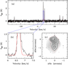 |
Fig. 1 (a) HC3N J = 2−1, F = 3− 2 spectrum of the peak position. Red lines show the Gaussian fitting. (b) Zoom-in of panel a showing line wing of HC3 N J = 2− 1, F = 3− 2. (c) Background is integrated map of HC3N J = 2−1, F = 3− 2. Black contours represent integration of red wing (6.75–7.08 km s−1) of HC3 N J = 2–1, F = 3–2 stepped from 60 to 90% by 10% of maximum value 0.14 K km s−1. The red contour denotes 3σ level (0.06 K km s−1) of HC3 N wing integration.The filled black square represents O point, and the black triangle represents P point (see text). The IRS is shown by the hexagonal star (Yen et al. 2014). Small black crosses show sampled points of Ku band observation. |
3.3 Lines at O point
Single point observations towards O point were made before the map. The highest S/Ns of the data at this point were compared to those of other points. The comparison enabled us to analyze the profile of molecular lines in detail. The lines at O point are thus also shown in Fig. 4. The left panel of Fig. 4 presents the spectral lines of HC3N, HC5N, HC7N, and C3 S in the Ku band. The right panel presents the spectral lines of C4H, CH3CCH, c-C3H2, and HC3N in 3 mm band.
The spectral peak of the HC7N J = 14−13 at O point shown in Fig. 4 seems to have a dip at the center with an S/N ≈ 3. The spectrum of HC7N J = 15−14 may also be split but interference of noise cannot be excluded. This was not seen in the spectrums of other CCMs in the Ku or 3 mm bands at O point. For the emission of C3 S J = 3−2, the TMB at O point is higher than that at P point, and therefore O point is adopted as the peak of the C3 S core.
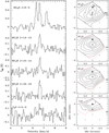 |
Fig. 2 Emissions of HC3N J = 2−1, HC5 N J = 6−5, and HC7N J = 14−13 as well as the C3S J = 3−2 in Ku band. Left: spectral lines at the P point. The emission of HC3N J = 2–1, F = 3–2 is shown in Fig. 1a. Right: intensity contours from 50 to 90% in steps of 10% of the peak value (see Table 2) for HC3N J = 2−1, F = 3− 2, HC5 N J = 6–5, and HC7N J = 14−13 as well as C3S J = 3− 2. Red contours represent 3σ of integrated emissions. The symbols are the same as those in Fig. 1c. |
3.4 Column density
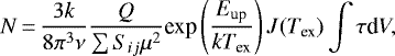
The column densities of the observed CCMs except C3 S were calculated from the integrated intensities oflines of P point. For C3S, parameters at O point are adopted. Assuming the gas is in local thermodynamic equilibrium (LTE) and the lines are optically thin, the column densities are calculated with the solution of the radiation transfer equation (Garden et al. 1991; Mangum & Shirley 2015)
 (1)
(1)
![\begin{eqnarray*}T_{\textrm{MB}}/\eta =f\frac{h\nu}{k} [({e^{\frac{h\nu}{kT_{\textrm{ex}}}}-1})^{-1}-({e^{\frac{h\nu}{kT_{\textrm{bg}}}}-1})^{-1}][1-e^{-\tau}] ,\end{eqnarray*}](/articles/aa/full_html/2019/07/aa34184-18/aa34184-18-eq2.png) (2)
(2)
where Sij, μ, and Q are the line strength, the permanent dipole moment, and the partial function, respectively, which are quoted from “Splatalogue”, and TMB is the main beam temperature, η is the efficiency of the main beam, and f is the beam filling factor, assumed to be unity.
The excitation temperature was calculated using different methods in this work for comparison. Using the hyperfine structure (HFS) fitting program in GILDAS/CLASS, we performed hyperfine structure fitting toward spectra of HC3N J = 2−1. The optical depth of the main component was obtained as τ = 0.45 ± 0.12 and an excitation temperature of 11.5 ± 1.0 K was derived through Eq. (2) with Tbg = 2.73 K and a beam filling factor of unity. We use the lines K = 0, 1, and 2 of CH3CCH J = 5−4 to derive therotational temperature Trot and a value of 12.6 ± 1.0 K was obtained (see the middle panel of Fig. 5). Since the K = 1,2 levels of CH3CCH J = 5–4 are easily thermalized and even more easily than NH3 (1,1) (2,2), the kinetic temperature Tk is assumed equal to Trot, 12.6 ± 1.0 K (Askne et al. 1984; Evans 1980).
Continuum data from far-infrared to sub-millimeter are available for the L1489 region4. The dust temperature(Td) and H2 column density were derived via modeling the PACS and SPIRE data of Herschel at 160, 250, 350, and 500 μm (see Table 3 and the right panel of Fig. 5) to a modified black body:
 (3)
(3)
where 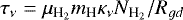 ; here
  = 2.8 is the mean molecular weight adopted from Kauffmann et al. (2008), mH is the mass of a hydrogen atom,
  is the column density, and Rgd = 100 is the ratio of gas to dust. The dust opacity κν can be expressed as a power law of frequency,
 (4)
(4)
with κν(850 GHz) = 5.9 cm2 g−1 adopted from Ossenkopf & Henning (1994). The free parameters are the dust temperature, dust emissivity index β, and column density. The fitting results give Td = 13.8 ± 0.2 K and  = (1.02 ± 0.07) × 1022 cm−2 with β =1.75.
These derived temperatures are listed in Table 4. The Td variation from the inner to outer parts of the core, which was model fitted from the SCUBA 850 μm image (Ford & Shirley 2011), is also listed in Table 4. These values are comparable with the kinetic temperature of L1527 (12.3 ± 0.8 K) and that of IRAS 15398-3359 (12.6 K; Sakai et al. 2008, 2009). Therefore, a unified excitation temperature of 12.6 K was adopted for calculating column densities and for further analyses.
For the column density of the detected species, only that of CH3CCH can be derived by analysis of multiple transitions at different energy levels. For other species including the hyperfine lines of HC5N and multiple rotation lines of HC7N, the upper level energies of the multiple lines are close to one another and this method is impractical. The average values of column densities calculated from multiple lines weighted by TMB/σ was therefore adopted as the species column density.
The Tex uncertainty will bring in about 10% error for calculation of column densities of all the species.
The column densities are listed in Table 2. The uncertainties of column densities are derived from errors of Tex and line integrated intensities. The column densities of our N-bearing molecules range from 1.4 × 10¹² to 4.5 × 1013 cm−2. Among all the detected molecules in the Ku band, C3S has the lowest column density, 0.8 × 1012 cm−2, which is much lower than those of starless cores such as TMC-1, L1544, and L1498 (Suzuki et al. 1992); this is also lower than that of the stellar core L1251A (Cordiner et al. 2011).
Observed and derived parameters.
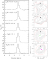 |
Fig. 3 Emissions of the transitions in the 3 mm band. Left: spectral lines of the P point. Right: emission intensity contours from 50 to 90% in steps of 10% of the peak value (see Table 2). C4H N = 9−8, J = 19/2−17/2 and C4 H N = 9−8, J = 17/2−15/2 are summed up and shown as C4H intensity contours. Red contours represent 3σ of integrated emissions. The symbols are the same as those in Fig. 1c. The green and pink filled triangles represent peak position of c-C3H2 J = 2−1 and HC3N J = 10−9 emission, respectively. |
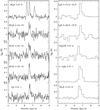 |
Fig. 4 Spectra at O position. Left: spectra at Ku band. Right: spectra at the 3 mm band detected with the 13.7 m telescope of PMO. |
4 Discussion
4.1 Carbon-chain molecule emission characteristics
The species C4H N = 9–8, J = 19/2–17/2, 17/2–15/2 and CH3CCH J = 5–4, K = 0, 1, 2 were detected in the WCCC source L1527 (Sakai et al. 2008). CH3CCH J = 5–4, K = 2 is the highest-excitation line detected in L1527. All of these lines were detected in the EMC. In the EMC, N-bearing species appear to be relatively abundant while C3S is very weak.
Figure 6 presents the CCM column densities of the EMC and L1527 as well as the five early carbon-chain-producing regions normalized by the values of TMC-1. One can see that the column densities of the species with high-energy excitation lines in the EMC and L1527 are close to each other. The CH3CCH column densities of the two cores are slightly higher than that of TMC-1 while their values of C4 H are lower than that of TMC-1. Among five starless cores, L1521B is the only one where the C4 H is detected. It is worth noting that the column density of C4H in L1521B is even higher than that of TMC-1. In this source the detected C4 H line is N = 2−1 J = 5∕2−3∕2, F = 2−1, 3−2 with an upper level energy of 1.4 K, which is much lower than those of lines detected in the EMC and L1527 (Hirota et al. 2004). However, the HC3N J = 10–9 with Eup 24.0 K was detected in the starless core L1498 (Tafalla et al. 2006). Since only the EMC and L1498 have this transition observed, it was not plotted on Fig. 6.
From Fig. 6 one can also see that among all the starless cores, the column densities of the N-bearing species in the EMC and L1527 are at the intermediate level. The HC3N column density in the EMC is higher than that of L1527. The N-bearing species seem to be abundant in WCCC sources in general. In the WCCC source IRAS 15398-3359, a very-high-energy excitation line of HC5N J = 32–31 with Eup 67.5 K was detected though the detection is tentative (Sakai et al. 2009). The HC3N column density in IRAS 15398-3359 is 1.5 × 1014 cm−2 (Wu et al., in prep.). In the massive core WCCC source NGC 7536 the HC5N column density is 1 × 1013 cm−2 which is derived from the detected line of HC5N J = 11–10 (Saul et al. 2015). The Eup of the HC5N J = 11–10 transition is 28.8 K.
As for the S-bearing species, Fig. 6 shows that the column density of the EMC is a little lower than that of L1527. However, C3 S column densities of both sources, about 6.5% (EMC) and 10% (L1527) of the TMC-1 value, respectively, are much lower than all of the compared early starless cores. It was recognized previously that S-bearing species are usually deficient in star-forming cores. A number of low-mass star-forming cores were examined for emissions of S-bearing CCMs by Suzuki et al. (1992). Results showed no or marginal detection for most protostellar cores and L1489 was taken as an example. In the EMC, the emission of C3 S J = 2−1 at P point is also marginally detected. Our C3S J = 3−2 map shows that the emission peak of C3 S J = 3−2 (O point) is separated from those of N-bearing species and NH3 (Myers et al. 1988), similar to the cases of L1498 and L1544. But even at the O point, the column density of the C3 S is still much lower than those of L1544 and L1498.
All these comparisons present the following characteristics of the EMC.
- 1.
Emissions of the species with high-energy excitation lines of the EMC are close to those of L1527. For these two sources the column densities of the species with high-energy excitation lines are comparable with those of TMC-1.
- 2.
For the N-bearing species, the column densities of the EMC and L1527 are at the medium level among all the samples.
- 3.
The column density of C3S of the EMC is close to that of L1527 but is much lower than those of all starless cores.
In short, the CCM emissions of the EMC are similar to those of L1527 but deviate from the early cold starless cores.
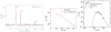 |
Fig. 5 Left: spectra of CH3CCH J = 5− 4, K = 0,1,2. Middle: rotation temperature diagram of CH3CCH. Right: SED of the L1489 IRS from the PACS 160 μm and SPIRE wavelengths of Herschel as well as SCUBA 850 μm. The filled squares represent the input fluxes. The line shows the best fitting of the gray-body model. |
Dust parameters.
Temperatures.
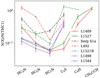 |
Fig. 6 Comparison between the CCM column densities of L1489 EMC and typical CCM rich sources, normalized by the values of TMC-1 (Kaifu et al. 2004; Suzuki et al. 1992). The source names are denoted in the lower-right corner with different colors, including starless cores Serpens South 1a (Serp S1a; Li et al. 2016), L492 (Hirota & Yamamoto 2006; Hirota et al. 2009), L1521B (Suzuki et al. 1992; Hirota et al. 2004), L1498 (Suzuki et al. 1992; Kuiper et al. 1996) and L1544 (Suzuki et al. 1992) as well as WCCC source L1527 (Sakai et al. 2008). The HC7 N column density of L1544 is derived from that of HC5N assuming the ratio of HC2n+1/HC2n+3 (n = 1,2) is constant (Suzuki et al. 1992). The N(C3S) of L1527 is deduced from column densities of C2S and the ratioof the C3S/C2S (Sakai et al. 2008; Suzuki et al. 1992). |
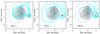 |
Fig. 7 Left: the HC3N core (gray-scale) and the NH3 (1,1) core (blue dashed lines, quoted from Myers et al. 1988) overlaid on the JCMT SCUBA 850 μm continuum data from JCMT proposal ID M97AN16 (Hogerheijde & Sandell 2000) (cyan contours, evenly stepped from 0.075 to 0.75 Jy beam−1 in log-scale). The gray and blue triangles denote the peaks of the EMC (P point) and NH3, respectively. The IRS is also marked on the map (hexagonal star). The blue and red wings of the CO (3− 2) outflow (blue solid and red dotted lines, quoted from Hogerheijde et al. 1998) and the medium infalling lobe (red solid line, quoted from Yen et al. 2014) were also overlaid on the figure. Middle: as in left panel except cyan contours representing Herschel SPIRE 500 μm continuum map, from 1.5 Jy beam−1 to 5 Jy beam−1 stepped by 0.3 Jy beam−1. Right: as in left panel except cyan contours representing Herschel SPIRE 250 μm continuum contours, from 1.5 to 5 Jy beam−1 stepped by 0.3 Jy beam−1. Fluxes around the IRS are centrally peaked but higher level contours are not shown. |
4.2 Core status and environment
L1489 is one of the 90 small visually opaque regions chosen from the Palomar Sky Atlas prints (Myers et al. 1983). NH3 (1,1) mapping presents a gas core which is about half an arcminute south of the high visual opacity and about one arcminute east of the IRAS 04016+2610, which was revealed as a Class I IRS (Myers et al. 1988, 1987). This region was also mapped with N2 H+ J = 1–0 (Caselli et al. 2002). The peak positions of the NH3 (1,1) and N2 H+ J = 1–0 map are closely coincident with our P point (1 arcmin east of L1489 IRS). These observations confirm that the EMC is dark and starless, similar to those early starless cores presented in Fig. 6.
The C2S distributions of L1498 and L1544 have a central hole which can be explained with infall and rotation (Hirota & Yamamoto 2006; Ohashi et al. 1999). In the EMC no sign of collapse or rotation has been detected so far and it is quiescent. At P point there is strong NH3 emission together with weak C3S emission, which may be related to the evolutional state of the core (Suzuki et al. 1992; Hirota & Yamamoto 2006).
The abundance ratios of NH3/C2S of TMC-1, L1521B, L492, L1498 and L1544 range from 2.9 to 25 (Hirota & Yamamoto 2006). For the EMC, using the NH3 column density of Myers et al. (1988) and the C2S column density estimated from C3 S emission with an average abundance ratio C2 S/C3S of 4.3 ± 0.9 derived from the data of starless cores including L1498, L1521B, TMC-1 and L1544 (Suzuki et al. 1992), the ratio of NH3/C2S is 289. This is one order of magnitude larger than the largest of the seven cores listed in Hirota & Yamamoto (2006). It is also larger than the NH3/C2S ratio of 37 for Serp S1a, which was derived from NH3 and C3S column densities with the ratio of C2 S/C3S 4.3 (Friesen et al. 2013; Li et al. 2016; Suzuki et al. 1992). Serp S1a has a more active and complex environment than starless cores in Taurus and infall was detected (Friesen et al. 2013). These indicate that the EMC has the latest evolutionary state among all the starless cores shown in Fig. 6.
A prominent difference between the EMC and other early starless cores is the temperature and the thermalisation of the gas. In TMC-1 the rotational temperature ranges from 4 to 8 K while the kinetic temperature ranges from 9 to 10 K (Kawaguchi et al. 1991; Kalenskii et al. 2004; Snyder et al. 2006; Sakai et al. 2008). The dust temperature is 10.5–12 K (Fehér et al. 2016) and 10.6 ± 0.1 K (Wu et al., in prep.). Serp S1a has a Tk 10.8 K derived from NH3 (1,1) (2,2) and 7 K was adopted as Tex (Friesen et al. 2013; Li et al. 2016). The Tex of L492 was derived as 6.4 K from HC3N and 8.3 K from CO, respectively (Hirota & Yamamoto 2006). L1521B has a Tex of 5.5–6.5 K and its TK is about 10 K (Hirota et al. 2004; Suzuki et al. 1992). The Tex of C3S of L1498 ranges from 5.5 to 10 K (Suzuki et al. 1992; Kuiper et al. 1996), and the Tk is 10 K derived from NH3 emission in this core. The Td of L1498 is 10 K (Tafalla et al. 2004). The Tex of L1544 is from 5 to 6.5 K (Suzuki et al. 1992) and TK derived from NH3 is ~ 10 K, and the Td of L1544 is also 10 K (Tafalla et al. 2002). In the EMC however, the Tex is 11.5 K derived from HC3N and Trot is 12.6 K from CH3CCH, which are similar to the Trot of C4 H2 (12.3 ± 0.8 K) and CH3CCH (13.9 K) for L1527 (Sakai et al. 2008). These comparisons show that the gas of the EMC is warmer and closer to thermalization status than those in early starless cores and comparable to that of L1527. These may explain why the carbon-chain molecular emissions in the EMC are similar to those of WCCC sources.
However, there is a fundamental difference in that L1527 contains a protostar which is the heating source of the core material (Goldreich & Kwan 1974; Sakai et al. 2008). For the EMC, there is no protostar inside, only an association with a protostellar object L1489 IRS at one arcminute to the west.
Figure 7 displays the images of 850, 500, and 250 μm continuum emissions as well as molecular line emissions in the L1489 region. One can see that the P point (black triangle), the centers of larger 850 μm continuum core, and the NH3 core (blue triangle) are close to each other but not overlaid exactly. Such deviation among peaks of different molecular line emission regions are very common in prestellar and stellar cores even in the TMC-1 region (Sánchez-Monge et al. 2014; Keown et al. 2016; Pratap et al. 1997). Cores of other molecular lines such as N2 H+ J = 1–0 and CS J = 3–2 are also coincident with the EMC (Caselli et al. 2002; Zhou et al. 1989). The weaker but larger core in the east of L1489 IRS shown in the SCUBA 850 μm map and the SPIRE 500 μm image covered the EMC entirely.
The L1489 IRS is a Class I source while the one in L1527 is a Class 0 object. The Lbol is 3.6–3.8 L⊙ for the L1489 IRS and 1.3–1.9 L⊙ for L1527, respectively (Kristensen et al. 2012; Chen et al. 1995). The Tbol of L1527 is 44 K (Kristensen et al. 2012; Chen et al. 1995), while the Tbol of the L1489 IRS is 200–283 K and more than five times of that of L1527 on average (Kristensen et al. 2012; Chen et al. 1995). The C4 H emission extends from the center part of the envelope to 5600 AU in L1527. High-energy excitation CCM lines in the EMC are possible to be excited, though L1489 IRS is located at the margins of the EMC since L1489 IRS is has relatively high bolometric luminosity and temperature. Further more, H2O 11,0 –10,1 observed with HIFI on Herschel presents an inverse P Cygni profile in L1527 but a P Cygni profile in L1489 IRS, indicating that L1489 IRS lacks an outer, cooler gas layer, which is in favor of the heating of its neighboring material.
From Fig. 7 one can see that at each wavelength, the strongest emission is around the IRS. The higher the frequency, the more the contours concentrate at the IRS. The tails of the contours of the 250 and 500 μm maps present a trajectory format starting from the IRS, which has not previously been seen in low-mass protostellar cores. These may be the evidence that the EMC is heated by the L1489 IRS. The size of the 250 μm emission region is 169.1 arcsec and Td from the spectral energy distribution (SED) fitting based on data of PACS-SPIRE bands is 13.8 K in the whole region.
The heating of L1489 IRS can be more significant considering the possible evolutionary history of the relationship between L1489 IRS and the EMC; they may be neighbors since the birth of L1489 IRS. However, another possibility may be that the IRS has moved away from the EMC center to the cloud margin, or it has dispersed the surrounding gas and has separated itself from the EMC (Harju et al. 1993; Wu et al. 2006). The influences of the L1489 IRS might what gives the EMC its WCCC characteristics.
However, WCCC began from reactions of C+ and sublimated CH4 from dust. A precondition is that the temperature needs to be ~30 K (Sakai et al. 2009). For L1527, the kinetic temperature is 20–30 K derived from the c-C3H2 43,2–42,1 line detected with the Plateau de Bure Interferometer (Sakai et al. 2010a). From the c-C3H2 and SO lines measured with ALMA with beam sizes 0.8′′ × 0.7′′ and 0.7′′ × 0.5′′ and analyzed with non-LTE large-velocity-gradient code, the kinetic temperatures of the c-C3H2 emitting region was found as 30 K at 100 AU (Sakai et al. 2014). The kinetic temperatures of L1527 measured from the interferometers are much higher than 13.9 K derived from the CH3CCH J = 5–4, K = 1,2 observed using NRO 45 m telescope with beam size ~20′′. These results present effects of telescope beams. The kinetic temperature of the EMC derived from CH3CCH J = 5–4, K = 0,1,2 detected with the PMO 13.7 m telescope with a beam size of 53′′ is 12.6 ± 1.0 K. The dust temperature fitted from JCMT and Herschel data is 13.8 ± 0.2 K. Both the values of the kinetic and dust temperature are comparable to those of L1527 measured with the NRO 45 m telescope. For the IRS sources, both the Lbol and Tbol of the L1489 IRS are higher than those of L1527. These comparisons indicate that in a smaller region within the EMC the kinetic temperaturemay be higher than the current results. Higher-resolution observations are needed to measure the temperature.
In the WCCC source L1527, CCMs of the prestellar phase could survive if the prestellar collapse is faster than that of other star-formingcores (Sakai et al. 2008). The EMC should have an early and a cold phase, like those starless cores shown in Fig. 6. No collapse or infall have been found in the EMC so far. The CCMs detected in the EMC may have survived from its early phase. In particular, the chemical activities of the CCMs seem to be related to their existence in the WCCC phase. Because of the different polarities, the N- and S-bearing species are more active than C4 H and CH3CCH and more likely to react with their partners. For example, the major loss route of C4 H is through reaction with C+ (Millar & Freeman 1984): C4 H+C+ → C +H, which has a rate coefficient of 2.0 ×10⁻⁹ cm3 at 10 K. While the reaction of HC3N with C+: HC3N+C+ → C3 HN++C has a rate coefficient of 8.7 ×10⁻⁹ cm3 at the same temperature (Leung et al. 1984). However, both species are formed from hydrocarbon ions and the reaction rates are not significantly different from one another (Leung et al. 1984). This suggests that the molecular species with high-energy excitation lines have a higher rate of survival than low-excitation lines, which might be a reason for the emissions of species with high-energy excitation lines in L1527 (Sakai et al. 2008) and the late core EMC. This may also be the reason for the detection of the HC3N J = 10–9 line with Eup 24.0 K in L1498 (Tafalla et al. 2006).
Besides the high-excitation lines and the N-bearing and S-bearing species discussed above, circular hydrocarbon c-C3H2 with TMB 1.72 K was also detected in the EMC. The species HC3N J = 10–9 with a high upper-level energy of 24.0 K is detected with TMB 0.63 K. Maps of all the detected species except for C3S show consistent emission peaks at about 1 arcmin east of the L1489 IRS. These results show that the EMC is an abundant CCM laboratory. Its comparable and contrasting conditions with the WCCC source L1527 and with early cold carbon-chain-producing regions may promote further CCM searches and help to constrain model analyses of CCMs.
5 Summary
Abundant carbon-chain molecules were detected toward the EMC of L1489 IRS, which is identified as a particular carbon-chain-producing region.
- 1.
With the TMRT, HC3N J = 2−1, HC5N J = 6–5, and HC7N J = 14–13, 15–14, 16–15 as well as C3S J = 3–2 were detected. The TMB of the hyperfine line J = 2–1 F = 3–2 of HC3N is 3.23 K. Five hyperfine lines of HC3N J = 2 − 1 were resolved. Hyperfine components of F = 7–6, F = 6–5, and F = 5−4 of HC5N J = 6 − 5 were resolved for the first time. The TMB of the three rotational lines of HC7N ranges from 0.25 to 0.32 K. The emission of C3S J = 3–2 is the weakest among the detected transitions. Using the PMO telescope, high-energy excitation lines including C4 H N = 9–8, J = 17/2–15/2, 19/2–17/2, CH3CCH J = 5–4, K =2, and HC3N J = 10–9 were detected. The highest upper-level energy is 41.1 K. All the transitions in Ku and 3 mm band are detected for the first time in the EMC of L1489 IRS.
- 2.
Maps of the observed transition lines were also obtained. Emission peaks of our detected lines except C3 S are all located at about 1′ east of the L1489 IRS, which is consistent with previously detected gas cores and the 850 μm continuum east core.
- 3.
The CCM column densities of the EMC were compared with those of TMC-1 together with five carbon-chain-producing regions in early phase (Serp S1a, L492, L1521B, L1498 and L1544) and WCCC source L1527. Results show that the column densities of the species with high-energy excitation lines including CH3CCH and C4 H in the EMC are close to those of L1527. The C3S column density of the EMC is slightly lower than that of L1527 but much lower than the five starless cores. The column densities of the N-bearing species are close to those of L1527, and the values of the both sources are at the intermediate level of the starless cores.
- 4.
Similarly to early carbon-chain-producing regions, the EMC is dark, starless, and quiescent. However, the EMC is rather at a late evolutionary stage (N(NH3)/N(C3S) = 289), and is warmer than starless carbon-chain-producing regions. On the other hand, the temperature and thermalization of the EMC are close to those of L1527, though L1527 is a protostellar core. These indicate that the EMC is very special among the carbon-chain-producing regions detected so far.
- 5.
The L1489 IRS has relatively high bolometric luminosity and temperature. The weaker but larger core to the east of L1489 IRS shown in the SCUBA 850 μm and the SPIRE 500 μm images covered the EMC completely. The tails of the contours of the 250 and 500 μm maps present a trajectory format starting from the IRS. The dust continuum emission area and the morphology of the contours show that the EMC is externally heated by the L1489 IRS.
Acknowledgements
We are grateful to the staff of PMO Qinghai Station and SHAO. We also thank Shanghuo Li, Kai Yang and Bingru Wang for their assistance during the observation period. This project was supported by the grants of National Key R&D Program of China No. 2017YFA0402600, NSFC Nos. 11433008, 11373009, 11373026, 11503035, 11573036, U1331116 and U1631237, and the Top Talents Program of Yunnan Province. This research used the facilities of the Canadian Astronomy Data Centre operated by the National Research Council of Canada with the support of the Canadian Space Agency.
References
- Askne, J., Hoglund, B., Hjalmarson, A., & Irvine, W. M. 1984, A&A, 130, 311 [NASA ADS] [Google Scholar]
- Avery, L. W., Broten, N. W., MacLeod, J. M., Oka, T., & Kroto, H. W. 1976, ApJ, 205, L173 [NASA ADS] [CrossRef] [Google Scholar]
- Bell, M. B., Feldman, P. A., Travers, M. J., et al. 1997, ApJ, 483, L61 [NASA ADS] [CrossRef] [Google Scholar]
- Benedettini, M., Pezzuto, S., Burton, M. G., et al. 2012, MNRAS, 419, 238 [Google Scholar]
- Benson, P. J., & Myers, P. C. 1989, ApJS, 71, 89 [NASA ADS] [CrossRef] [Google Scholar]
- Brinch, C., Crapsi, A., Hogerheijde, M. R., & Jørgensen, J. K. 2007, A&A, 461, 1037 [NASA ADS] [CrossRef] [EDP Sciences] [Google Scholar]
- Broten, N. W., Oka, T., Avery, L. W., MacLeod, J. M., & Kroto, H. W. 1978, ApJ, 223, L105 [NASA ADS] [CrossRef] [Google Scholar]
- Bussa, S., & VEGAS Development Team. 2012, Amer. Astron. Soc. Meet. Abstr., 219, 446.10 [NASA ADS] [Google Scholar]
- Caselli, P., Benson, P. J., Myers, P. C., & Tafalla, M. 2002, ApJ, 572, 238 [NASA ADS] [CrossRef] [Google Scholar]
- Chen, H., Myers, P. C., Ladd, E. F., & Wood, D. O. S. 1995, ApJ, 445, 377 [NASA ADS] [CrossRef] [Google Scholar]
- Cordiner, M. A., Charnley, S. B., Buckle, J. V., Walsh, C., & Millar, T. J. 2011, ApJ, 730, L18 [NASA ADS] [CrossRef] [Google Scholar]
- Evans, II, N. J. 1980, in Interstellar Molecules, ed. B. H. Andrew, IAU Symp., 87, 1 [NASA ADS] [Google Scholar]
- Fehér, O., Tóth, L. V., Ward-Thompson, D., et al. 2016, A&A, 590, A75 [NASA ADS] [CrossRef] [EDP Sciences] [Google Scholar]
- Ford, A. B., & Shirley, Y. L. 2011, ApJ, 728, 144 [NASA ADS] [CrossRef] [Google Scholar]
- Friesen, R. K., Medeiros, L., Schnee, S., et al. 2013, MNRAS, 436, 1513 [NASA ADS] [CrossRef] [Google Scholar]
- Fuller, G. A., & Myers, P. C. 1993, ApJ, 418, 273 [NASA ADS] [CrossRef] [Google Scholar]
- Garden, R. P., Hayashi, M., Hasegawa, T., Gatley, I., & Kaifu, N. 1991, ApJ, 374, 540 [NASA ADS] [CrossRef] [Google Scholar]
- Goldreich, P., & Kwan, J. 1974, ApJ, 189, 441 [NASA ADS] [CrossRef] [Google Scholar]
- Guilloteau, S., & Lucas, R. 2000, in Imaging at Radio through Submillimeter Wavelengths, eds. J. G. Mangum & S. J. E. Radford, ASP Conf. Ser., 217, 299 [NASA ADS] [Google Scholar]
- Harju, J., Walmsley, C. M., & Wouterloot, J. G. A. 1993, A&AS, 98, 51 [NASA ADS] [Google Scholar]
- Herbst, E., Smith, D., & Adams, N. G. 1984, A&A, 138, L13 [NASA ADS] [Google Scholar]
- Hirahara, Y., Suzuki, H., Yamamoto, S., et al. 1992, ApJ, 394, 539 [NASA ADS] [CrossRef] [Google Scholar]
- Hirota, T., & Yamamoto, S. 2006, ApJ, 646, 258 [NASA ADS] [CrossRef] [Google Scholar]
- Hirota, T., Ito, T., & Yamamoto, S. 2002, ApJ, 565, 359 [NASA ADS] [CrossRef] [Google Scholar]
- Hirota, T., Maezawa, H., & Yamamoto, S. 2004, ApJ, 617, 399 [NASA ADS] [CrossRef] [Google Scholar]
- Hirota, T., Ohishi, M., & Yamamoto, S. 2009, ApJ, 699, 585 [NASA ADS] [CrossRef] [Google Scholar]
- Hirota, T., Sakai, T., Sakai, N., & Yamamoto, S. 2011, ApJ, 736, 4 [NASA ADS] [CrossRef] [Google Scholar]
- Hogerheijde, M. R., & Sandell, G. 2000, ApJ, 534, 880 [NASA ADS] [CrossRef] [Google Scholar]
- Hogerheijde, M. R., van Dishoeck, E. F., Blake, G. A., & van Langevelde H. J. 1998, ApJ, 502, 315 [NASA ADS] [CrossRef] [PubMed] [Google Scholar]
- Irvine, W. M., Ziurys, L. M., Avery, L. W., Matthews, H. E., & Friberg, P. 1988, Astrophys. Lett. Commun., 26, 167 [NASA ADS] [Google Scholar]
- Kaifu, N., Ohishi, M., Kawaguchi, K., et al. 2004, PASJ, 56, 69 [NASA ADS] [CrossRef] [Google Scholar]
- Kalenskii, S. V., Slysh, V. I., Goldsmith, P. F., & Johansson, L. E. B. 2004, ApJ, 610, 329 [NASA ADS] [CrossRef] [Google Scholar]
- Kauffmann, J., Bertoldi, F., Bourke, T. L., Evans, II, N. J., & Lee, C. W. 2008, A&A, 487, 993 [NASA ADS] [CrossRef] [EDP Sciences] [Google Scholar]
- Kawaguchi, K., Kaifu, N., Ohishi, M., et al. 1991, PASJ, 43, 607 [NASA ADS] [Google Scholar]
- Keown, J., Schnee, S., Bourke, T. L., et al. 2016, ApJ, 833, 97 [NASA ADS] [CrossRef] [Google Scholar]
- Kristensen, L. E., van Dishoeck, E. F., Bergin, E. A., et al. 2012, A&A, 542, A8 [NASA ADS] [CrossRef] [EDP Sciences] [Google Scholar]
- Kroto, H. W., Kirby, C., Walton, D. R. M., et al. 1978, ApJ, 219, L133 [NASA ADS] [CrossRef] [Google Scholar]
- Kuiper, T. B. H., Langer, W. D., & Velusamy, T. 1996, ApJ, 468, 761 [NASA ADS] [CrossRef] [PubMed] [Google Scholar]
- Lada, C. J. 1985, ARA&A, 23, 267 [NASA ADS] [CrossRef] [Google Scholar]
- Leung, C. M., Herbst, E., & Huebner, W. F. 1984, ApJS, 56, 231 [NASA ADS] [CrossRef] [Google Scholar]
- Li, J., Shen, Z.-Q., Wang, J., et al. 2016, ApJ, 824, 136 [NASA ADS] [CrossRef] [Google Scholar]
- Lovas, F. J. 2004, J. Phys. Chem. Ref. Data, 33, 177 [NASA ADS] [CrossRef] [Google Scholar]
- Mangum, J. G., & Shirley, Y. L. 2015, PASP, 127, 266 [NASA ADS] [CrossRef] [Google Scholar]
- Markwick, A. J., Millar, T. J., & Charnley, S. B. 2000, ApJ, 535, 256 [NASA ADS] [CrossRef] [Google Scholar]
- Matthews, H. E., Irvine, W. M., Friberg, P., Brown, R. D., & Godfrey, P. D. 1984, Nature, 310, 125 [NASA ADS] [CrossRef] [Google Scholar]
- Millar, T. J., & Freeman, A. 1984, MNRAS, 207, 405 [NASA ADS] [Google Scholar]
- Müller, H. S. P., Schlöder, F., Stutzki, J., & Winnewisser, G. 2005, J. Mol. Struct., 742, 215 [NASA ADS] [CrossRef] [Google Scholar]
- Myers, P. C., Linke, R. A., & Benson, P. J. 1983, ApJ, 264, 517 [NASA ADS] [CrossRef] [Google Scholar]
- Myers, P. C., Fuller, G. A., Mathieu, R. D., et al. 1987, ApJ, 319, 340 [NASA ADS] [CrossRef] [Google Scholar]
- Myers, P. C., Heyer, M., Snell, R. L., & Goldsmith, P. F. 1988, ApJ, 324, 907 [NASA ADS] [CrossRef] [Google Scholar]
- Ohashi, N., Lee, S. W., Wilner, D. J., & Hayashi, M. 1999, ApJ, 518, L41 [Google Scholar]
- Olano, C. A., Walmsley, C. M., & Wilson, T. L. 1988, A&A, 196, 194 [NASA ADS] [Google Scholar]
- Ossenkopf, V., & Henning, T. 1994, A&A, 291, 943 [NASA ADS] [Google Scholar]
- Pickett, H. M., Poynter, R. L., Cohen, E. A., et al. 1998, J. Quant. Spectr. Rad. Transf., 60, 883 [NASA ADS] [CrossRef] [Google Scholar]
- Pratap, P., Dickens, J. E., Snell, R. L., et al. 1997, ApJ, 486, 862 [Google Scholar]
- Sakai, N., Sakai, T., Hirota, T., & Yamamoto, S. 2008, ApJ, 672, 371 [NASA ADS] [CrossRef] [Google Scholar]
- Sakai, N., Sakai, T., Hirota, T., Burton, M., & Yamamoto, S. 2009, ApJ, 697, 769 [NASA ADS] [CrossRef] [Google Scholar]
- Sakai, N., Sakai, T., Hirota, T., & Yamamoto, S. 2010a, ApJ, 722, 1633 [NASA ADS] [CrossRef] [Google Scholar]
- Sakai, N., Shiino, T., Hirota, T., Sakai, T., & Yamamoto, S. 2010b, ApJ, 718, L49 [NASA ADS] [CrossRef] [Google Scholar]
- Sakai, N., Sakai, T., Hirota, T., et al. 2014, Nature, 507, 78 [NASA ADS] [CrossRef] [Google Scholar]
- Sánchez-Monge, Á., Beltrán, M. T., Cesaroni, R., et al. 2014, A&A, 569, A11 [NASA ADS] [CrossRef] [EDP Sciences] [Google Scholar]
- Saul, M., Tothill, N. F. H., & Purcell, C. R. 2015, ApJ, 798, 36 [Google Scholar]
- Shan, W.-Y., Lu, H.-Z., & Shen, S.-Q. 2012, Phys. Rev. B, 86, 125303 [NASA ADS] [CrossRef] [Google Scholar]
- Snyder, L. E., Hollis, J. M., Jewell, P. R., Lovas, F. J., & Remijan, A. 2006, ApJ, 647, 412 [NASA ADS] [CrossRef] [Google Scholar]
- Suzuki, H., Yamamoto, S., Ohishi, M., et al. 1992, ApJ, 392, 551 [NASA ADS] [CrossRef] [Google Scholar]
- Tafalla, M., Myers, P. C., Caselli, P., Walmsley, C. M., & Comito, C. 2002, ApJ, 569, 815 [NASA ADS] [CrossRef] [Google Scholar]
- Tafalla, M., Myers, P. C., Caselli, P., & Walmsley, C. M. 2004, A&A, 416, 191 [NASA ADS] [CrossRef] [EDP Sciences] [Google Scholar]
- Tafalla, M., Santiago-García, J., Myers, P. C., et al. 2006, A&A, 455, 577 [NASA ADS] [CrossRef] [EDP Sciences] [Google Scholar]
- Taniguchi, K., Saito, M., Sridharan, T. K., & Minamidani, T. 2018, ApJ, 854, 133 [NASA ADS] [CrossRef] [Google Scholar]
- Turner, B. E. 1971, ApJ, 163, L35 [NASA ADS] [CrossRef] [Google Scholar]
- Wang, J. Q., Yu, L. F., Zhao, R. B., et al. 2015, Acta Astron. Sin., 56, 63 [NASA ADS] [Google Scholar]
- Wang, Y., Chang, Q., & Wang, H. 2019, A&A, 622, A185 [NASA ADS] [CrossRef] [EDP Sciences] [Google Scholar]
- Winnewisser, G., & Walmsley, C. M. 1978, A&A, 70, L37 [NASA ADS] [Google Scholar]
- Wu, Y., Zhang, Q., Chen, H., et al. 2005, AJ, 129, 330 [NASA ADS] [CrossRef] [Google Scholar]
- Wu, Y., Zhang, Q., Yu, W., et al. 2006, A&A, 450, 607 [NASA ADS] [CrossRef] [EDP Sciences] [Google Scholar]
- Yen, H.-W., Takakuwa, S., Ohashi, N., et al. 2014, ApJ, 793, 1 [NASA ADS] [CrossRef] [Google Scholar]
- Zhang, X.-Y., Zhu, Q.-F., Li, J., et al. 2017, A&A, 606, A74 [NASA ADS] [CrossRef] [EDP Sciences] [Google Scholar]
- Zhou, S., Wu, Y., Evans, II, N. J., Fuller, G. A., & Myers, P. C. 1989, ApJ, 346, 168 [NASA ADS] [CrossRef] [Google Scholar]
- Ziurys, L. M. 2006, Proc. Natl. Acad. Sci., 103, 12274 [NASA ADS] [CrossRef] [Google Scholar]
All Tables
All Figures
|
Fig. 1 (a) HC3N J = 2−1, F = 3− 2 spectrum of the peak position. Red lines show the Gaussian fitting. (b) Zoom-in of panel a showing line wing of HC3 N J = 2− 1, F = 3− 2. (c) Background is integrated map of HC3N J = 2−1, F = 3− 2. Black contours represent integration of red wing (6.75–7.08 km s−1) of HC3 N J = 2–1, F = 3–2 stepped from 60 to 90% by 10% of maximum value 0.14 K km s−1. The red contour denotes 3σ level (0.06 K km s−1) of HC3 N wing integration.The filled black square represents O point, and the black triangle represents P point (see text). The IRS is shown by the hexagonal star (Yen et al. 2014). Small black crosses show sampled points of Ku band observation. |
| In the text | |
|
Fig. 2 Emissions of HC3N J = 2−1, HC5 N J = 6−5, and HC7N J = 14−13 as well as the C3S J = 3−2 in Ku band. Left: spectral lines at the P point. The emission of HC3N J = 2–1, F = 3–2 is shown in Fig. 1a. Right: intensity contours from 50 to 90% in steps of 10% of the peak value (see Table 2) for HC3N J = 2−1, F = 3− 2, HC5 N J = 6–5, and HC7N J = 14−13 as well as C3S J = 3− 2. Red contours represent 3σ of integrated emissions. The symbols are the same as those in Fig. 1c. |
| In the text | |
|
Fig. 3 Emissions of the transitions in the 3 mm band. Left: spectral lines of the P point. Right: emission intensity contours from 50 to 90% in steps of 10% of the peak value (see Table 2). C4H N = 9−8, J = 19/2−17/2 and C4 H N = 9−8, J = 17/2−15/2 are summed up and shown as C4H intensity contours. Red contours represent 3σ of integrated emissions. The symbols are the same as those in Fig. 1c. The green and pink filled triangles represent peak position of c-C3H2 J = 2−1 and HC3N J = 10−9 emission, respectively. |
| In the text | |
|
Fig. 4 Spectra at O position. Left: spectra at Ku band. Right: spectra at the 3 mm band detected with the 13.7 m telescope of PMO. |
| In the text | |
|
Fig. 5 Left: spectra of CH3CCH J = 5− 4, K = 0,1,2. Middle: rotation temperature diagram of CH3CCH. Right: SED of the L1489 IRS from the PACS 160 μm and SPIRE wavelengths of Herschel as well as SCUBA 850 μm. The filled squares represent the input fluxes. The line shows the best fitting of the gray-body model. |
| In the text | |
|
Fig. 6 Comparison between the CCM column densities of L1489 EMC and typical CCM rich sources, normalized by the values of TMC-1 (Kaifu et al. 2004; Suzuki et al. 1992). The source names are denoted in the lower-right corner with different colors, including starless cores Serpens South 1a (Serp S1a; Li et al. 2016), L492 (Hirota & Yamamoto 2006; Hirota et al. 2009), L1521B (Suzuki et al. 1992; Hirota et al. 2004), L1498 (Suzuki et al. 1992; Kuiper et al. 1996) and L1544 (Suzuki et al. 1992) as well as WCCC source L1527 (Sakai et al. 2008). The HC7 N column density of L1544 is derived from that of HC5N assuming the ratio of HC2n+1/HC2n+3 (n = 1,2) is constant (Suzuki et al. 1992). The N(C3S) of L1527 is deduced from column densities of C2S and the ratioof the C3S/C2S (Sakai et al. 2008; Suzuki et al. 1992). |
| In the text | |
|
Fig. 7 Left: the HC3N core (gray-scale) and the NH3 (1,1) core (blue dashed lines, quoted from Myers et al. 1988) overlaid on the JCMT SCUBA 850 μm continuum data from JCMT proposal ID M97AN16 (Hogerheijde & Sandell 2000) (cyan contours, evenly stepped from 0.075 to 0.75 Jy beam−1 in log-scale). The gray and blue triangles denote the peaks of the EMC (P point) and NH3, respectively. The IRS is also marked on the map (hexagonal star). The blue and red wings of the CO (3− 2) outflow (blue solid and red dotted lines, quoted from Hogerheijde et al. 1998) and the medium infalling lobe (red solid line, quoted from Yen et al. 2014) were also overlaid on the figure. Middle: as in left panel except cyan contours representing Herschel SPIRE 500 μm continuum map, from 1.5 Jy beam−1 to 5 Jy beam−1 stepped by 0.3 Jy beam−1. Right: as in left panel except cyan contours representing Herschel SPIRE 250 μm continuum contours, from 1.5 to 5 Jy beam−1 stepped by 0.3 Jy beam−1. Fluxes around the IRS are centrally peaked but higher level contours are not shown. |
| In the text | |
Current usage metrics show cumulative count of Article Views (full-text article views including HTML views, PDF and ePub downloads, according to the available data) and Abstracts Views on Vision4Press platform.
Data correspond to usage on the plateform after 2015. The current usage metrics is available 48-96 hours after online publication and is updated daily on week days.
Initial download of the metrics may take a while.