| Issue |
A&A
Volume 627, July 2019
|
|
|---|---|---|
| Article Number | A173 | |
| Number of page(s) | 23 | |
| Section | Stellar structure and evolution | |
| DOI | https://doi.org/10.1051/0004-6361/201834081 | |
| Published online | 18 July 2019 | |
Masses and ages for metal-poor stars
A pilot programme combining asteroseismology and high-resolution spectroscopic follow-up of RAVE halo stars⋆,⋆⋆
1
Leibniz-Institut für Astrophysik Potsdam (AIP), An der Sternwarte 16, 14482 Potsdam, Germany
e-mail: marica.valentini@oapd.inaf.it
2
Osservatorio Astronomico di Padova, INAF, Vicolo dell’Osservatorio 5, 35122 Padova, Italy
3
Instituto de Astrofísica e Ciências do Espaço, Universidade do Porto, CAUP, Rua das Estrelas, 4150-762 Porto, Portugal
4
School of Physics and Astronomy, University of Birmingham, Edgbaston, Birmingham B15 2TT, UK
5
Stellar Astrophysics Centre, Department of Physics and Astronomy, Aarhus University, 8000 Aarhus C, Denmark
6
LESIA, Observatoire de Paris, PSL Research University, CNRS, Université Pierre et Marie Curie, Université Paris Diderot, 92195 Meudon, France
7
Departamento de Astrofísica, Universidad de La Laguna, 38206 Tenerife, Spain
8
Instituto de Astrofísica de Canarias, C/ Vía Láctea s/n, La Laguna 38205, Tenerife, Spain
9
IRFU, CEA, Université Paris-Saclay, 91191 Gif-sur-Yvette, France
10
AIM, CEA, CNRS, Université Paris-Saclay, Université Paris Diderot, Sorbonne Paris Cité, 91191 Gif-sur-Yvette, France
Received:
13
August
2018
Accepted:
26
May
2019
Context. Very metal-poor halo stars are the best candidates for being among the oldest objects in our Galaxy. Samples of halo stars with age determination and detailed chemical composition measurements provide key information for constraining the nature of the first stellar generations and the nucleosynthesis in the metal-poor regime.
Aims. Age estimates are very uncertain and are available for only a small number of metal-poor stars. We present the first results of a pilot programme aimed at deriving precise masses, ages, and chemical abundances for metal-poor halo giants using asteroseismology and high-resolution spectroscopy.
Methods. We obtained high-resolution UVES spectra for four metal-poor RAVE stars observed by the K2 satellite. Seismic data obtained from K2 light curves helped improve spectroscopic temperatures, metallicities, and individual chemical abundances. Mass and ages were derived using the code PARAM, investigating the effects of different assumptions (e.g. mass loss and [α/Fe]-enhancement). Orbits were computed using Gaia DR2 data.
Results. The stars are found to be normal metal-poor halo stars (i.e. non C-enhanced), and an abundance pattern typical of old stars (i.e. α and Eu-enhanced), and have masses in the 0.80−1.0 M⊙ range. The inferred model-dependent stellar ages are found to range from 7.4 Gyr to 13.0 Gyr with uncertainties of ∼30%−35%. We also provide revised masses and ages for metal-poor stars with Kepler seismic data from the APOGEE survey and a set of M4 stars.
Conclusions. The present work shows that the combination of asteroseismology and high-resolution spectroscopy provides precise ages in the metal-poor regime. Most of the stars analysed in the present work (covering the metallicity range of [Fe/H] ∼ −0.8 to −2 dex) are very old >9 Gyr (14 out of 19 stars), and all of the stars are older than >5 Gyr (within the 68 percentile confidence level).
Key words: stars: fundamental parameters / asteroseismology / stars: abundances
Atmospheric parameters, abundances, and the linelist are only available at the CDS via anonymous ftp to cdsarc.u-strasbg.fr (130.79.128.5) or via http://cdsarc.u-strasbg.fr/viz-bin/qcat?J/A+A/627/A173
© ESO 2019
1. Introduction
The Milky Way halo is a key component in understanding the assembly history of our Galaxy. The halo is composed by stars that were accreted during mergers as well as stars that formed in situ (e.g. Helmi et al. 1999, 2018), and is suggested to be one of the oldest components of our Galaxy, (e.g. Jofré & Weiss 2011; Kalirai 2012; Kilic et al. 2019). In addition, metal-poor halo giant stars enshrine information on when star formation began, on the nature of the first stellar generation, and on the chemical enrichment timescale in the Galactic halo (Cayrel et al. 2001; Chiappini 2013; Frebel & Norris 2015). A comprehensive understanding of the Galactic halo can be obtained only when combining precise stellar chemical abundances, kinematics, and ages. While detailed chemical information can be obtained via high-resolution spectroscopic analysis and precise kinematics is being provided by astrometric missions such as Gaia, the determination of reliable stellar ages (i.e. ages that are precise and unbiased) is still a challenging task, especially in the case of red giants.
Before the confirmation of solar-like oscillations in red giant stars (De Ridder et al. 2009), ages were estimated only for a limited sample of nearby field stars, either by model-dependent techniques such as isochrone fitting or empirical methods such as nucleo-cosmo-chronometry. The age determination via the classic isochrone-fitting method has always been hampered by the fact that in the red giant locus the isochrones clump together, which leads to a large degeneracy. This degeneracy leads to age uncertainties easily above 80% for the oldest stars (e.g. da Silva et al. 2006; Feuillet et al. 2016). The few metal-poor field halo stars with a better age determination than the isochrone fitting are determined by the nucleo-cosmo-chronometry technique (mostly derived using the Th-232 and U-238 ratio), and these stars have old ages (Cayrel et al. 2001; Cowan et al. 2002; Hill et al. 2002, 2017; Sneden et al. 2003; Ivans et al. 2006; Frebel et al. 2007; Placco et al. 2017). These old ages seem to confirm the expectations that metal-poor halo objects are among the oldest objects in our Galaxy. Although the nucleo-cosmo-chronometry method is more precise than isochrone fitting in the case of red giants, it is not a viable solution for all stars. The method requires high-resolution and high signal-to-noise (S/N) spectra in the blue region of the spectrum (S/N > 300 at ∼390 nm), and high r-process enhancement to allow for the presence of strong, and sufficiently measurable, U and Th lines.
Asteroseismology of red giant stars has, in recent years, demonstrated to provide precise masses for such stars, and therefore ages (Casagrande et al. 2016; Anders et al. 2017; Silva Aguirre et al. 2018). Solar-like oscillations are commonly summarised by two parameters: Δν (average frequency separation) and νmax (frequency of maximum oscillation power). These two quantities provide precise mass (precision of about 10%) and radius (precision of about 3%), using the so-called seismic scaling relations, and an additional information on stellar temperature (Teff) (Miglio et al. 2013; Casagrande et al. 2014; Pinsonneault et al. 2014). Since for red giants the stellar masses are a good proxy for stellar age, it is possible to determine a model-dependent age with a precision that can be better than 30% depending on the quality of the seismic information (Davies & Miglio 2016). More precise ages, with an error ∼15%, can be obtained via Bayesian methods combining seismic information with Gaia data and information on the stellar evolutionary stage (Rodrigues et al. 2017, and references therein).
Since the age determination using asteroseismology relies on the mass-age relation that red giants follow, this means that the method is biased by any event that changes the stellar mass, such as mass accretion from a companion or stellar mergers (blue stragglers or stars rejuvenated by accretion, e.g. Boffin et al. 2015) or mass loss. One way to look for mass accretion events from a companion is to look for radial velocity, photometric variations, or chemical signs of accretion (e.g. high carbon and s-process enhancements; Beers & Christlieb 2005; Abate et al. 2015). The effect of mass loss can be minimised by looking at stars in the low-RGB phase, in which the effect of mass loss is smaller compared to red clump stars (Anders et al. 2017). The first study to determine masses for a sample of metal-poor halo giants with both seismic information (from Kepler; Borucki et al. 2010) and chemistry from high-resolution APOGEE (Majewski et al. 2017) spectra, was by Epstein et al. (2014). The authors used scaling relations at face value and reported masses larger (M > 1 M⊙) than what would be expected for a typical old population. Similar results were obtained by Casey et al. (2018), also using scaling relations for three metal-poor stars. These findings led to the need for further tests of the use of asteroseismology in the low metallicity regime. Miglio et al. (2016) analysed a group of red giants in the globular cluster M4 ([Fe/H] = −1.10 dex and [α/Fe] = 0.4 dex) with seismic data from K2 mission (Howell et al. 2014). These authors found low seismic masses compatible with the old age of the cluster, hence suggesting that seismic masses and radii estimates would be reliable in the metal-poor regime provided that a correction to the Δν scaling relation is taken into account for red giant branch (hereafter RGB) stars. The correction presented in Miglio et al. (2016) is a correction that is theoretically motivated based on the computation of radial mode frequencies of stellar modes.
In this work, we present a first set of four stars identified as metal poor ([Fe/H] ∼ −2 dex) in the RAVE (Radial Velocity Experiment, Steinmetz et al. 2006) survey, for which we have seismic information from the K2 mission and high-resolution spectra. The paper is organised as follows: in Sect. 2 we describe how the stars have been selected and observed. The seismic light curve analysis and the determination of atmospheric parameters and abundances from stellar spectra are described in Sect. 3. In Sect. 4 we derive radii, masses, and ages for our stars using both PARAM (a Bayesian tool for deriving stellar properties, Rodrigues et al. 2017) and seismic scaling relations. We recompute masses for the Epstein et al. (2014) and M4 (Miglio et al. 2016) samples. We also analyse the offsets and uncertainties introduced by different seismic pipelines, erroneous assumptions in temperature, [α/Fe] enhancements, and mass loss. Distances and orbits of the stars are derived in Sect. 5, using Gaia DR2 parallaxes and proper-motions. In Sect. 6 we discuss each of the four RAVE stars in light of their chemistry, age, and orbital properties. Section 7 summarises our conclusions and provides an outlook.
2. Observations
2.1. K2
Targets analysed in this works belong to K2 mission campaigns 1 and 3. The K2 Campaign 1 field (C1), centred at RA 11h35m46s Dec +01°25′00″ (l = 265, b = +58), was observed from 30 May 2014 to 21 August 2014, and contains one metal-poor RAVE star. The K2 Campaign 3 field (C3), centred at RA 22h26m40s Dec −11°25′02″ (l = 51, b = −52), was observed from 14 November 2014 to 03 February 2015, contains three RAVE metal-poor giants. The RAVE targets were observed as part of the “The K2 Galactic Archaeology Program Campaign” (C1–C3 proposal GO1059, and described in Stello et al. 2015).
Light curves were obtained using the same approach as described in Sect. 3 of Valentini et al. (2017).
2.2. Target selection
In C1 and C3 K2 fields there are a total of 376 RAVE targets for which solar-like oscillations have been detected. Following the joint spectroscopic and seismic analysis described in Valentini et al. (2017) we identified four stars expected to have metallicities [Fe/H] ≤ −1.5 dex. The spectra of the metal-poor targets are visible in Fig. 1.
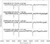 |
Fig. 1. Spectra taken by the RAVE survey of the 4 metal-poor stars presented in this paper. Spectra are normalised and corrected for radial velocity; the Fe content labelled comes from the analysis of RAVE spectra using the same method as in Valentini et al. (2017). |
The RAVE spectra cover a narrow spectral interval (8410−8795 Å) at intermediate resolution (R ∼ 7500), which combined with the low metallicity of the targets (few detectable lines, as visible in Fig. 1) make the traditional spectroscopic analysis challenging: the atmospheric parameters may suffer of degeneracies and offsets. Using the t-SNE projection, Matijevič et al. (2017), we confirmed that the four stars were, indeed, metal poor. The t-SNE projection (t-Distribution Stochastic Neighbour Embedding, van der Maaten & Hinton 2008) is an algorithm that, when applied to spectra, provides a low-dimensional projection of the spectrum space and isolates objects that present similar morphology. In our case, as visible in Fig. 2, metal-poor stars clump in the top left region of the projection. In the figure ∼420 000 RAVE spectra with S/N > 10 are projected; the RAVE stars in K2 C1 and C3 are represented as empty circles. The four stars that fall into the very metal-poor island (top right) are the metal-poor giants analysed in the present work.
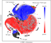 |
Fig. 2. t-SNE projection of ∼420 000 RAVE spectra. The scaling in both direction is arbitrary, therefore the units on the axes are omitted. The colour scale corresponds to the gravity of the stars as computed by Kunder et al. (2017). Giants are shown in red and dwarfs in blue. Lighter shaded hexagons include fewer stars than darker ones. Over-plotted black dots indicate locations of RAVE stars in K2 Campaigns 1,3. Illustrated as stars are the RAVE-K2 objects studied in the present work, which fall in the metal-poor locus of the diagram. |
2.3. Gaia DR2
The four stars are in Gaia DR2 (Gaia Collaboration 2016, 2018). Parallaxes, proper motions, and flags are listed in Table 1. The duplicated_source flag is listed as Dup.
Gaia DR2 data and seismic data for the 4 RAVE metal-poor stars studied in this work.
Star S1 (Epic ID: 201359581) has a “duplicated_source” flag = true, meaning that this source presented more than one detection and only one entry was kept. This means that the star had observational or processing problems, leading to possible erroneous astrometric or photometric solution. This same star has an “astrometric_excess_sigma” ≥ 2 that, combined with “astrometric_excess_noise” flag > 0, indicates large astrometric errors and an untrustworthy solution. For this same star the Gaia DR2 radial velocity has an error of 5.17 km s−1, hence larger than the ∼0.8 km s−1 expected for a star of that temperature and brightness.
Star S2 (Epic ID: 205997746) has a “Priam_flag” indicating a silver photometry quality and a lower quality in the temperature, radius and luminosity solutions, while the rest of the stars in the sample have a better, golden, photometry quality.
For S1 (201359581), we did not consider the ages and masses derived by taking into account the Gaia DR2 information. In addition, we consider the solutions for S2 (205997746) of lower quality respect to the other two stars, S3 (206034668) and S4 (206443679). We use the Gaia DR2 proper motions when computing orbits for our stars in Sect. 5, with the exception of S1, for which we use UCAC-5 (Zacharias et al. 2017) proper motions.
Gaia DR2 parallax, ϖ, can be used for deriving the surface gravity as follows:
We derived log(g)ϖ for the stars of our sample, assuming the bolometric correction (BC) as in Casagrande & VandenBerg (2014, 2018), using Ks magnitudes and assuming stellar masses of 0.9 M⊙ and temperatures as derived from the analysis of the high-resolution spectra. Errors were calculated via propagation of uncertainties and varying stellar masses from 0.8 to 2.2 M⊙ (a typical red giant star mass range). We also took into account the effect of the different offsets in the ϖ, considering the zero point correction (Lindegren et al. 2018) and the offset pointed out by Zinn et al. (2019). Thus we considered an offset effect that varies ϖ within (ϖ − 0.3) and (ϖ + 0.2). Resulting gravities and their uncertainties are listed together with the stellar parameters obtained from spectroscopy (see next sections) in Table 4.
2.4. High-resolution spectra
The UV-Visual Echelle Spectrograph (UVES) high-resolution spectra of our targets were collected in the period 99D1, using UVES-CD 3 set-up (Dekker et al. 2000). Spectra have a resolving power of ∼110 000 and cover ∼4170−6200 Å spectral range. Observing date, exposure time, and S/N of spectra are listed in Table 2.
Coordinates and set-up of the ESO-UVES observations of the stars.
3. Data analysis
3.1. Seismic data
Very metal-poor stars typically have large radial velocities that induce a Doppler shift of observed frequencies. Although small, this shift can be larger than the precision on asteroseismic frequencies. In this work we use the average seismic parameters Δν and νmax. Because Δν is a frequency difference and because the precision on νmax is much lower than for individual mode frequencies the Doppler correction does not need to be applied to asteroseismic average parameters (Davies et al. 2014).
In order to quantify the impact of the different seismic inputs on the estimates of the mass and age of our stars, we first considered the Δν and νmax measurements coming from four different seismic pipelines:
-
COR: This method is adopted for CoRoT and Kepler stars (Mosser & Appourchaux 2009; Mosser et al. 2011). In a first step, the average frequency separation, Δν, is measured from the autocorrelation of the time series computed as the Fourier spectrum of the filtered Fourier spectrum of the signal. The significance of the result is checked using a statistical test based on the H0 hypothesis.
-
GRD: This pipeline is based on fitting a background model to the data (Davies et al. 2016). This model H (Kallinger et al. 2014) is comprised of two Harvey profiles, a Gaussian oscillation envelope, and an instrumental noise background. For the estimate of νmax the central frequency of the Gaussian component is considered. The median and standard deviations are used to summarise the normal-like posterior probability density for νmax. To estimate the average frequency separation a model was fitted to the power spectrum (Davies & Miglio 2016).
-
YE: This approach has three stages. First, a S/N spectrum as a function of frequency is created by dividing the power spectrum by a heavily smoothed version of the raw power spectrum. The second step consists in using a combination of H0 and H1 hypothesis for detecting oscillation power in segments of the S/N spectrum. If a segment shows detection of oscillations power, then νmax and Δν are detected as a third step (Hekker et al. 2010; Elsworth et al. 2017).
-
A2Z: This pipeline measures a first estimate of Δν using the same method as COR. The value νmax is measured by fitting a Gaussian on top of the background to the power spectrum. Then Δν is recomputed from the power spectrum of the power spectrum and by considering only the central orders of the spectrum centred on the highest radial mode (Mathur et al. 2010, 2011). In contrast to the previous pipelines, this measured a value for Δν only for two of the four targets and provided significantly larger error bars for νmax.
We then checked that the different pipelines were in agreement for the four stars, as showed in Fig. 3. As we are dealing with a small number of stars and since the four pipelines are in agreement, we can perform a star-by-star analysis of the goodness of the seismic values. From a visual inspection, as visible in Appendix A, it appears that: (i) A2Z pipeline is providing Δν with very large uncertainties; (ii) YE and GRD pipelines provide a νmax value that appears shifted respect to the expected value for star S1 and S2, respectively (see Fig. A.1). As shown by previous works (e.g. Lillo-Box et al. 2014; Pérez Hernández et al. 2016), using individual frequencies for deriving Δν is more precise than the method presented above. The individual frequencies fitting exercise is difficult to perform for K2 light curves because of the short duration of the K2 runs. For this reason the use of the universal pattern is preferred, as in Mosser et al. (2011), which uses detailed information of the whole oscillation pattern (Mosser et al. 2011). This dedicated analysis provides refined values of the global seismic parameters with smaller uncertainties. This choice is also justified by the tests performed in Hekker et al. (2012). For these reasons we therefore adopted Δν from the COR pipeline as our preferred value.
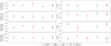 |
Fig. 3. Δν and νmax as measured by different pipelines. Each colour (blue, magenta, red, and green) corresponds to a different pipeline (COR, GRD, A2Z, and YE; see appendix). The values plotted in black correspond to a further test using COR with inflated uncertainties (BM_N). |
An additional test has been performed for RGB stars in the α-rich APOGEE-Kepler (APOKASC Pinsonneault et al. 2018) sample. Individual mode frequencies have been measured for ≈1000 stars and then a comparison between Δν measured from individual frequencies with the Δν measured by COR pipeline had been performed. A small (≲1%) difference between Δν as determined by COR and Δν determined from individual radial-mode frequencies is found (Davies et al., in prep.), supporting our choice for COR values. This is also relevant because the Δν determined from individual mode frequencies is closer to the Δν given in the stellar models adopted in PARAM, which is the tool we used the tool to derive mass, radii, and ages. We additionally considered the seismic values from GRD pipeline, which has error bars in Δν and νmax compatible with the COR pipeline and with the data quality (see more details in Appendix A).
To gain a better comprehension of the impact of the use of a global error coming from considering all the pipelines we also adopted a fifth set of Δν and νmax (BM_N), where the Δν and νmax are from the COR pipeline but with inflated errors that consider the dispersion of the pipelines respect to COR values, i.e.
where x = Δν or νmax. The adopted seismic values, COR and BM_N, are listed in Table 1 (the complete set of seismic values are in Table A.1) and a comparison of the different sets of Δν and νmax is shown Fig. 3.
We compared the Δν and νmax of our sample with the Δν and νmax distribution of the APOKASC sample. The high quality of the APOKASC sample makes it the perfect benchmark to provide a first glance on the masses expected for our objects. Figure 4 shows that our four stars fall in the region where the less massive stars are located.
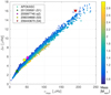 |
Fig. 4. Δν and νmax distribution of the 4 stars studied in this work. The Δν-νmax distribution distribution of the APOKASC sample is colour coded following the mass. |
3.2. RAVE spectra analysis
We performed the analysis of the RAVE spectra following the method described in Valentini et al. (2017, Sect. 4). We iteratively derived atmospheric parameters by fixing the gravity to the seismic value, log(g)S. As a starting point for deriving Teff, we used the infra-red flux method (IRFM) temperature published in RAVE-DR5 (Kunder et al. 2017), allowing for variations as large as 250 K. This analysis was performed using the GAUFRE pipeline (Valentini et al. 2013).
The seismic gravity we used is defined as
where the following solar values are adopted: νmax, ⊙ = 3090 μHz, Δν⊙ = 135.1 μHz, log(g)⊙ = 4.44 dex, and Teff, ⊙ = 5777 K (Huber et al. 2011).
Atmospheric parameters and abundances derived from RAVE spectra are listed in Table 3. Abundances were derived under local thermodynamic equilibrium (LTE). The chemical abundances obtained from RAVE spectra suggest that the four stars are α-enhanced with [α/Fe] ∼ 0.3 dex. On the other hand the individual abundance ratios of [Mg/Fe], [Si/Fe], and [Ti/Fe] are significantly discrepant for the different stars. We note that the [Fe/H] values reported in Table 3 are not corrected for non-local thermodynamic equilibrium (NLTE) effects. We return to this point when discussing the abundance ratios obtained from high-resolution spectra.
Radial velocity, atmospheric parameters, and abundances of the metal-poor RAVE stars in K2 Campaigns 1 and 3, as derived from RAVE spectra.
3.3. UVES spectra analysis
We analysed the high-resolution UVES spectra using the GAUFRE pipeline to retrieve Teff, log(g), and [Fe/H] iteratively with the seismic information on log(g) using Eq. (3). The analysis was performed with the GAUFRE module GAUFRE_EW, which derives atmospheric parameters via ionisation and excitation equilibrium using the equivalent widths (EW) of FeI and FeII lines, MARCS model atmospheres (Gustafsson et al. 2008), and the silent version of MOOG 20172. For the sake of comparison we derived atmospheric parameters also employing the classical method imposing excitation and ionisation equilibrium using FeI and FeII lines; the results are listed as Teff, Cl and log(g)Cl in Table 4.
Atmospheric parameters and radial velocities of the stars as obtained from Gaia DR2 and from high-resolution UVES spectra.
The error in Teff was calculated by considering that the range of Teff within the Fe I abundances was independent from the line excitation potential (slope equal to zero) and by varying log(g) and vmic within errors. The error in log(g) was calculated via propagation of uncertainty when the adopted log(g) was derived using asteroseismology (Eq. (3)). When log(g) was measured via the classic method (ionisation equilibrium of Fe I and Fe II), the uncertainty was derived by varying Teff, vmic, and [Fe/H] by their uncertainty because the values are interdependent.
Abundances of different chemical elements were derived using MOOG 2017, in the updated version properly treating Rayleigh scattering (Sobeck et al. 2011)3. For the abundances analysis, an ad hoc model atmosphere with the same atmospheric parameters found by GAUFRE was created via interpolation using MARCS models. The linelist was constructed using the linelists in Roederer et al. (2014a), Hill et al. (2002), and was implemented, when necessary, with line parameters retrieved from VALD DR4 database (Ryabchikova et al. 1997, 2015; Kupka et al. 1999, 2000; Piskunov et al. 1995). The C abundance was derived via fitting the A-X CH band head at ∼4000−4300 Å. Line parameters were taken from Masseron et al. (2014). We measured the abundances of the following alpha elements: Mg, Si, Ca, and Ti. The NLTE corrections for Ti are taken from the work of Bergemann (2011). In addition we measured the abundances of several iron peak elements (Cr, Mn, Fe, Ni, Cu, Zn, and Ga). For Fe we adopted the line-by-line NLTE corrections provided by Bergemann et al. (2012). The NLTE corrections for Mn are taken from Bergemann & Gehren (2008). Line-by-line corrections for Fe and Mn are taken from a user friendly interface available on-line4. As an indicator of r-process enrichment we measured abundances of Eu and Gd. As s-process markers we measured Sr and Ba.
Final abundances are listed Table 5 (for more details see Appendix B). The uncertainties on abundances provided in Table 5 (and in Table B.1) were calculated considering: the internal error of the fit, the errors on Teff and log(g), and the error on continuum normalisation. The error on the fit is provided by MOOG itself. We computed the impact of Teff and log(g) uncertainties by creating different model atmospheres by varying atmospheric parameters within the errors. Error on continuum normalisation has been taken into account by creating, for each stellar spectrum, ten different continuum normalisations and then analysing them. The error listed in Table 5 is the sum in quadrature of these three different errors. In Fig. 5 we compare the abundance pattern of the four RAVE stars with that of CS 31082−001 (dotted grey curve), which is considered to be a typical pure r-process enriched star (Spite et al. 2018). The abundances for CS 31082−001 were taken from Roederer et al. (2014b).
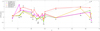 |
Fig. 5. Chemical abundance pattern [X/Fe] for the four metal-poor stars studied in this work. As a reference, the abundances pattern of the r-process enriched star CS 31082−001 are plotted as a dark grey line (abundances from Roederer et al. 2014b). |
Summary of the abundances of the stars of this work.
The four stars are clearly enhanced in core collapse (SN type II) nucleosynthetic products (such as Mg, Si, and Eu), as one would expected to be the case for old stars. However, the range in α enhancement is very large, and it is not correlated with metallicity. S1, S2, and S4 can be classified as r-I stars (i.e. stars with 0.3 ≤ [Eu/Fe] ≤ 1 and [Ba/Eu]<, Christlieb et al. 2004), while S3 is clearly Ba-enhanced. The low C enhancement and the low [Ba/Fe] ratios (with only the exceptional case of S3) suggest a minor contribution from AGB-mass transfer (if any).
The values obtained from the analysis of high-resolution UVES spectra for [Mg/Fe], [Si/Fe], and [Ti/Fe] can now be compared with those reported in Table 3 obtained from the RAVE spectra. In most of the cases the discrepancies are above the quoted error bars; this is probably due to the combination of the lower resolution and shorter spectral coverage of RAVE spectra, which leads to undetected line blends and the presence of very few lines per element. The [α/Fe] ratios coming from high-resolution UVES spectra show a large variation. Enhancements for S2 and S4 seem systematically larger than those of S1 and S3.
In Fig. 6 the atmospheric parameters in this work (from RAVE and UVES spectra) are compared with the literature values presented in RAVE-DR5 (calibrated values), RAVE-on (Casey et al. 2017, where the stellar parameters were obtained by using a data-driven approach). It is worth noticing that the RAVE-on catalogue misplaced these red giants in metallicity and/or gravity. This misclassification might be due to the training sample adopted in Casey et al. (2017), consisting mostly of APOGEE red giants, which are mostly metal rich. In Fig. 6 is also visible that for the star 201359581 the temperature obtained with the Valentini et al. (2017) method is ∼350 K higher than that measured from the high-resolution spectrum. This is a consequence of the fact that the starting Teff adopted was erroneous. For stars S2, S3, and S4, there is a good agreement between the temperatures estimated from the RAVE and high-resolution analysis spectra upon the use of the seismic gravity. The agreement is also seen in metallicity, where the most discrepant case, S4, is our most metal-poor star for which the non-local thermodynamic equilibrium (NLTE) corrections are more important; we took into account NLTE effects when analysing UVES spectra. Two important results can be extracted from Fig. 6: first, by combining the RAVE spectra with seismic gravities it is possible to reach precise stellar parameters similar to what is obtained from high-resolution spectra (see the agreement between the black dots (UVES) and red points (RAVE) for three out of the four stars). Second, the high-resolution analysis has confirmed that one of the stars has metallicity [Fe/H] < −2. The difficulty in determining the metallicity of such metal-poor objects from moderate resolution spectra covering a rather short wavelength range, without the benefit of the extra seismic information, is clearly illustrated by the discrepant metallicities found by RAVE DR5 and RAVE-on. When comparing the high-resolution results with the values published in Valentini et al. (2017) upon the use of K2 information, where the temperatures and gravities are consistent, we find a good agreement.
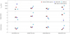 |
Fig. 6. Atmospheric parameters of the sample of metal-poor stars, as taken from literature and this work: RAVE spectra and seismic parameters (red squares), RAVE-DR5 (blue triangles), RAVE-on (cyan triangles), and ESO high-resolution spectra and seismic parameters (black circles). |
4. Mass and age determination
We performed mass determinations using two different methods: a direct method using scaling relations and a Bayesian fitting using the PARAM code (Rodrigues et al. 2017). Masses derived using scaling relation differ from those from PARAM (see discussion in Rodrigues et al. 2017). We now illustrate this difference for the case of our four metal-poor stars. The resulting masses from the two methods are summarised in Table 6.
Seismic mass and radius calculated using scaling relations (Teff measured from UVES spectra), and mass, radius, and age derived using PARAM, for the 4 metal-poor RAVE stars in K2 Campaigns 1 and 3.
Mass estimate using scaling relations. For our computations using the scaling relations we adopted as input Δν and νmax from the COR pipeline and the Teff measured from the UVES spectra. The scaling relations are in the form
where the solar values adopted are the same those listed in Sect. 2, and Δν = 135.1 μHz. The uncertainties on the masses and radii are calculated using propagation of uncertainties, under the assumption of uncorrelated errors.
Mass estimate using PARAM. For deriving ages and masses via Bayesian inference we adopted the latest version of the PARAM code. The new version of the code uses Δν that has been computed along MESA (Modules for Experiments in Stellar Astrophysics, Paxton et al. 2011) evolutionary tracks, plus νmax computed using the scaling relation. The following modifications were implemented with respect to the version described in Rodrigues et al. (2017). First, we extended the grid towards the metal-poor end down to [Fe/H] = −3 dex by calculating evolutionary tracks for [Fe/H] = −2.0 and −3.0 dex, with He enrichment computed according Rodrigues et al. (2017). Second, we took α-elements enrichment into account by converting the observed chemical composition into a solar-scaled equivalent metallicity. We investigated the solutions provided by PARAM when setting an upper limit to the age at 14 Gyr and without age upper limit; the latter helps us to understand the shape of the probability density function (PDF) of mass and age.
4.1. Mass-loss and alpha-enhanced tracks
In addition PARAM provides an estimate for stellar distance and luminosity, L (listed in Table 7). The luminosities provided by PARAM were used to construct Fig. 7, where we placed our stars in the temperature-luminosity diagram. The figure shows a set of MESA evolutionary tracks for masses 0.8 and 1.0 M⊙ at two different metallicities, Z = 0.00060 and Z = 0.00197. In the same figure the four stars are also plotted, together with the track, in the νmax-Teff (middle panel) and Δν-Teff planes. The stars of our sample are most likely low-luminosity RGB stars, which are not expected to undergo significant mass loss. The evolutionary state of star S1 (201359581), on the other hand, is more uncertain since it is located close to the RGB bump (dashed line); also following Fig. 1 of Khan et al. (2018), S1 can be core He burning, RGB, or early AGB. The evolutionary status of this star becomes relevant when it comes to discussing the reliability of age estimates since stars in the red clump or early AGB phases suffer of significant mass loss, which hampers the mass (and hence age) determination. Finally, since our stars are well located below the bump (with a flag on S1 that is a borderline case), we consider their abundances not affected by an extra mixing process that happens at the bump and early AGB stage.
Seismic distances and luminosities calculated using scaling relations, PARAM, distances obtained from Gaia parallaxes (both using the classical 1/ϖ and Bailer-Jones et al. 2018), distance calculated using StarHorse (Queiroz et al. 2018), and luminosity provided by Gaia DR2.
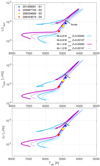 |
Fig. 7. Top panel: position in the temperature – luminosity diagram of the 4 RAVE stars of this work (nomenclature following Table 1). Evolutionary tracks at masses M = 0.8 and 1.0 M⊙, at two different metallicities (Z = 0.00060 and 0.00197) are plotted. Middle panel: position in the temperature – νmax diagram of the four RAVE stars of this work, same tracks as top panel. Bottom panel: position in the temperature – Δν diagram of the four RAVE stars of this work, same tracks as top panel. Error bars of the plotted quantities are of the size of the points. |
Because the adopted MESA stellar tracks in Rodrigues et al. (2017) assumed the Grevesse & Noels (1993) solar mixture for the metals, we adopted the α-enhancement correction to convert [Fe/H] into [M/H] using the formula from Salaris et al. (1993), which was updated with the relative mass fraction of elements from OPAL tables5,
![$$ \begin{aligned} \mathrm{[M/H]}^\mathrm{chem}= \mathrm{[Fe/H]}+ \log {\left( C \times 10^{[\alpha /\mathrm{Fe}]}+(1-C)\right)}, \end{aligned} $$](/articles/aa/full_html/2019/07/aa34081-18/aa34081-18-eq50.gif)
where C = 0.684.
This is a necessary step, given that all our stars are α-enhanced. We tested the effectiveness of this assumption by comparing two PARSEC track sets (from MS to RGB tip), which are also provided for α-enhanced cases. In Appendix C, we compare one track computed for [α/Fe] = +0.4 dex and [Fe/H] = −2.15, and one not α-enhanced, but with the corresponding metallicity following Eq. (6) ([Fe/H] = −1.86). The test shows that the deviation in age between the tracks has its maximum at the RGB tip in the mass regime of our stars. This deviation is of the order of 1−2%, a smaller effect respect to the typical age uncertainty. We derived mass and ages by adopting first the atmospheric parameters derived from RAVE spectra and then for the atmospheric parameters obtained from UVES spectra. We also computed mass and ages using the different seismic inputs discussed in Sect. 2 (COR and BM_N). This strategy allows us to see the impact of different precision in the atmospheric parameters and seismic parameters. Results are summarised in Table E.1. Results obtained with the high-resolution input for temperature, metallicity, and an averaged [α/Fe] (computed as ([Mg/Fe]+[Si/Fe]+[Ca/Fe])/3) are in Fig. 8 and in Fig. E.2. In these figures it is visible that the PDF of masses and ages obtained with the seismic values with BM_N seismic values are broad and, in the case of 205997746, double peaked. This is a consequence of the inflated error in BM_N, caused by blindly combining all the spectroscopic pipelines. This shows that, when dealing with a detailed analysis of individual stars, a star-by-star approach for testing the performances of each seismic pipeline is a necessary step to increase the precision of mass and age determination.
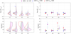 |
Fig. 8. Left column: violin plot of the PDFs of mass (top) and age (bottom). The right magenta shaded PDF is derived using the parameters from BM_N seismic set of parameters; the new errors take into account dispersion between pipelines and the PDFs on the left of the violin are calculated using seismic parameters from COR pipeline (black line, grey shaded) and varying the Teff of +100 K (dashed blue line) or −100 K (dotted red line). Right column: modes and 68 percentile errorbar of masses (top) and ages (bottom) of the 4 stars of this work. Magenta points indicate values computed using BM_N seismic values, black diamonds indicate the values derived using COR seismic values, and red and blue triangles indicate values obtained using COR seismic values and varying the Teff of −100 and +100 K, respectively. |
Our adopted final values of stellar mass and radius, derived using COR seismic input and UVES spectra, are shown in Table 6, where we also show, for comparison, the results obtained directly from the scaling relations. The mass and ages of PARAM are obtained adopting a mass-loss value derived from Reimers (1975) law with an efficiency parameter of η = 0.2. We adopted this value since it is in agreement with what was measured in Miglio et al. (2012) by comparing the asteroseismic masses of red clump stars and red giants in the old open clusters NGC 6791 and NGC 6819. The error associated with the mode value of radius, mass, and age derived using PARAM is calculated as the shortest credible interval with 68 per cent of the PDF. Masses derived with scaling relations (Eq. (4)) are larger than those derived using PARAM by circa 30%. This is because of the correction needed to Δν (see Miglio et al. 2016), which leads to a more accurate mass estimation for red giants. In PARAM this correction is not necessary. The code can, in fact, derive the theoretical Δν directly by interpolation, since this quantity has been estimated along each evolutionary track.
4.2. Using luminosities from Gaia DR2 to further constrain PARAM
In the work of Rodrigues et al. (2017) the adoption of the intrinsic stellar luminosity, L, derived using Gaia parallaxes leads to a significant improvement into the mass and age determination (from an error of 5% in mass and 19% in age to 3% and 10%, respectively). These estimates were based on high-quality Kepler seismic data and very precise atmospheric parameters. In addition, the uncertainties on luminosity were assumed to be 3%, from Gaia end-of-the-mission performances. Gaia DR2 still does not reach this precision and offsets in ϖ have to be taken into account. Nevertheless we calculated mass, radius, and age using the additional information on L, calculated from parallax and discovered the shape of the PDFs were affected, suggesting some tension with the input luminosities.
Instead of using the luminosities tabulated in Gaia DR2, we considered the weighted mean of the L calculated from Ks, I, and V magnitudes, considering BC provided by Casagrande & VandenBerg (2014, 2018) 6 and the reddening derived from Schlegel et al. (1998) maps. Errors on L were calculated via error propagation; the error on BC was calculated via Monte Carlo simulation of 100 points for each star. Luminosities are listed in Table 7 and show ∼15% uncertainties, but the 3% end of mission expectation is not shown. We thus opted for not using luminosities as an extra constraint in our calculations of mass and radius.
4.3. Uncertainties
To better understand the systematics that may affect the age determination using PARAM, we performed several tests under different assumptions:
-
We determined ages and masses for each set of seismic parameters provided by different pipelines.
-
We used atmospheric parameters from RAVE and UVES spectra.
-
We considered five different [α/Fe] abundances, 0.0, 0.1, 0.2, 0.3, 0.4 dex, when using atmospheric parameters derived from RAVE spectra, for each set of seismic parameters. Since the low resolution and limited wavelength interval of RAVE may affect the measured alpha content of the stars, we wanted to quantify the impact of an erroneous [α/Fe].
-
We considered two different mass loss efficiency parameters, η = 0.2 and 0.4. We performed this test for each set of seismic data adopted.
-
We varied the Teff of ±100 K; this shift simulates the effect of a difference in temperature that may exist between the various methods for measuring this temperature change.
-
We tested the impact of the precision on Teff, by adopting as input error a value two times the spectroscopic value. Resulting masses and ages are listed in Table E.1 in the rows labelled “COR2σTeff”.
-
We tested the introduction of an upper limit on the age. Resulting masses and ages are listed in Table E.1 in the rows labelled “CORage lim.”.
It is worth noting that the effects of these tests depend on the position of the star on the HR diagram and on its evolutionary stage. Each locus of the HR diagram is populated by different tracks and with different levels of crowdedness.
The variation on α content has no significant effect, providing a mass spread on average of 0.01 M⊙ and of 0.3 Gyr in age (see Figs. D.1 and D.2). As a general behaviour, when the α enrichment increases the mass slightly decreases and the age increases.
The underestimation of Teff of 100 K leads to a variation in mass and age on average of −10% and +30%, respectively. As expected, when the temperature increases, the mass increases and the age decreases, the opposite happens when the temperature decreases. This effect is more visible for the most metal-poor and hottest stars.
The adoption of an inflated error on Teff, two times the nominal spectroscopic error, leads to no sensible change in the mass and age determination. When adopting a seismically determined Teff, we take advantage of using a Teff that is consistent with the seismic parameters themselves. In the case of an inaccurate Teff, as for S1 using RAVE spectra, the solution is misleading and PARAM shows tensions in the posterior PDFs (see Fig. E.1).
The adoption of a mass-loss parameter η = 0.4 leads to a mass increase of only 2% and an age reduction of 4% in mass and age with respect to the values derived with η = 0.2 (see Figs. D.1 and D.2). As discussed in Anders et al. (2017) and Casagrande et al. (2016), the effect of mass loss is more significant for red clump stars than for RGB stars. Three of the four stars studied in this work are consistent with the RGB classification (see Fig. 7), so our results appear consistent with their findings.
Setting a uniform prior on age with an upper limit has a consequence on the shapes of the PDFs of ages. This is the reason why, in some cases, for the oldest stars of the sample, the PDF of the age appears truncated at the upper limit, as visible in Fig. E.2. Although not considering an upper limit on the age at 14 Gyr would not represent the information that we have about the age of the Universe, removing the age limit allows the PDF to extend to older ages, so we can better understand its shape and therefore the goodness of the age determination (e.g. multiple peaked PDF). As visible in Fig. E.2 and listed in Table E.1, the removal or adoption of an upper age limit has little consequence on the resulting mass and ages.
4.4. Masses and ages for two previously studied samples and comparison with our sample
We compared the masses of our stars with the masses previously determined in the literature for metal-poor field giants in the APOKASC sample (Epstein et al. 2014) and for giants in the globular cluster M4 (Miglio et al. 2016) using asteroseismic information as well. We also recomputed masses and ages for the two literature samples using PARAM in the same set-up used for the RAVE metal-poor stars analysed in this work.
The APOKASC metal-poor giants. For the APOKASC targets of Epstein et al. (2014) we adopted atmospheric parameters and their uncertainties from APOGEE-DR14 (Abolfathi et al. 2018) together with Δν and νmax obtained by the COR pipeline from Kepler light curves; this choice is necessary to guarantee homogeneity in our sample. The atmospheric parameters of APOGEE-DR14 differ from those adopted by Epstein et al. (2014), since that work used previous ASPCAP releases. The input parameters we used in PARAM are given in Table 8, where the metallicities [M/H] are computed with Eq. (6) to take into account the [α/Fe]-enhancement. The PARAM code provided mass and age for each star of the Epstein et al. (2014) work. We did not consider the results for star E14-S5 since the resulting a posteriori Teff, νmax, and Δν were not in agreement with the input values (see Appendix E for an example), indicating the presence of erroneous input parameters. The masses we obtained are smaller with respect to the original values of Epstein et al. (2014) who reported masses obtained using scaling relations. The new masses are also in agreement with the masses we obtained for the four RAVE stars (see Fig. 10 top panel). The differences in masses between the Epstein et al. (2014) estimates and ours are consistent with the fact that the scaling relation masses are systematically larger than those computed by PARAM for RGB stars (as previously discussed, see Table 6). The two samples together provide a better coverage of the metal-poor [Fe/H] regime. Masses of the Epstein et al. (2014) sample have been already recomputed by Sharma et al. (2016), Pinsonneault et al. (2018), and Yu et al. (2018), taking into account Δν corrections derived from stellar models. In Fig. 9, we compared the masses of the Kepler metal-poor stars of Epstein et al. (2014) with those computed in this work, Pinsonneault et al. (2018), and Yu et al. (2018); the latter work considered the values corresponding to their evolutionary status. The masses agree within errors. On the other hand, Yu et al. (2018) masses are in general always larger than those we computed in this work, thereby resulting into younger ages. This might be the result of the different set of atmospheric parameters adopted by the authors.
Input atmospheric parameters for the Epstein et al. (2014) stars and PARAM results of mass and age.
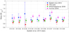 |
Fig. 9. Mass and age comparison for the 9 stars presented in Epstein et al. (2014; blue diamonds) with the values derived in this work (red circles), in Pinsonneault et al. (2018; green triangles) and Yu et al. (2018; magenta triangles). Stars are indexed as in Table 8. |
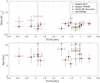 |
Fig. 10. Mass and ages of RGB stars in the metal-poor regime for a) four metal-poor RAVE stars with K2 seismic oscillations presented in this work (red diamonds); b) nine APOKASC the objects from Epstein et al. (2014) (original values as empty black circles; our new determination using PARAM and APOGEE-DR14 atmospheric parameters and abundances are shown as filled red circles), and c) seven stars in M4 from Miglio et al. (2016) recomputed with PARAM in this work (yellow triangles). |
Red giants in the M4 globular cluster. We also provide a similar comparison for seven M4 stars previously studied by Miglio et al. (2016) for which K2 seismic information were available. This sample is an ideal benchmark for testing our method since a reliable and precise age can be measured for globular clusters. In this case the temperature was obtained from (B − V) colour (corrected) as in Casagrande & VandenBerg (2014), assuming a temperature uncertainty of 100 K. The input parameters adopted in this case are summarised in Table 9. Our masses and ages determinations are consistent with the original values of Miglio et al. (2016) who, despite using the scaling relations, took the necessary correction for RGB stars into account. With the exception of one outlier (M4–S6), the stars provide an age for the globular cluster of ∼11.01 ± 2.67 Gyr, which was derived with the weighted mean based on the mean error, ∼11.80 ± 2.58 Gyr, when considering all the stars; this agrees with the age measured from isochrone fitting of 13 Gyr (or with the 12.1 ± 0.9 Gyr; Hansen et al. 2004, age measured from the white dwarf cooling sequence). The PDF of mass and age for the individual stars of M4 are plotted in Fig. F.1 and compared with the literature values.
Figure 10 summarises the ages and masses obtained in the present work for the three datasets (i.e. four RAVE, eight APOKASC, and seven M4 stars). In this figure we plot the ages and masses estimates for the four stars obtained using the COR pipeline seismic inputs consistent with the seismic inputs in Tables 8 and 9 of the other two samples analysed in this work. All the 19 stars plotted in the figure (filled symbols) are compatible with masses below one solar mass (top panel). Most of these halo objects are consistent with being very old, and none is younger than ∼7 Gyr. Moreover, our results show that it is possible to estimate ages for metal-poor giants with seismic information, not only from Kepler, but also from the K2 less precise light curves.
Input atmospheric parameters for the stars analysed in the M4 globular cluster Miglio et al. (2016) adopted in PARAM and resulting mass and age.
5. Distances and orbits
In this section we compute distances and orbits for the RAVE stars studied in this work. As a sanity check, we first compare distances estimates with five different methods, namely:
-
scaling relation;
-
PARAM distances derived using UVES atmospheric parameters and COR seismic values;
-
direct Gaia DR2 parallax;
-
StarHorse pipeline (Queiroz et al. 2018), using photometry and Gaia DR2 data, assuming a parallax zero-point correction of 0.52 mas (Zinn et al. 2019);
-
distances provided by Bailer-Jones et al. (2018).
Distances obtained with scaling relations were derived using the expression of Miglio et al. (2013), using the reddening as measured from Schlegel et al. (1998), i.e.

where d is in parsec, mbol is the apparent bolometric magnitude of the star, and Mbol, ⊙ the absolute solar bolometric magnitude. Bolometric corrections were adopted from Casagrande & VandenBerg (2018). Errors are calculated using propagation of uncertainty. Distances calculated using the different methods listed above are summarised in Table 7.
The different distances are in broad agreement. In particular, SH distances assuming a parallax zero point of −0.52 mas (Zinn et al. 2019) are in good agreement with those obtained from PARAM. In Table 10 the SH estimate extinctions for the four stars are given and compared with values from the literature. In the rest of our analysis we adopt the PARAM distances.
Reddening values for each stars as calculated from Schlegel et al. (1998), PARAM, and COR seismic values, StarHorse Queiroz et al. (2018) (spectroscopic atmospheric parameters and Gaia parallaxes) and Green et al. (2018).
Orbit parameters were calculated using GALPY (Bovy 2015)7. We adopted a Galactic potential (MWpotential2014) and a solar radius of 8.3 kpc. We adopted PARAM distances and, when available, Gaia proper motions (see Tables 1 and 7). In the case of 201359581 (S1) we adopted PARAM distances and UCAC 5 (Zacharias et al. 2017) proper motions, since the Gaia astrometric solution is not reliable. Errors on orbit parameters were calculated via the Monte Carlo approach, simulating 1000 stars per object with velocity, distance, and proper motions varying within errors. Results are summarised in Table 11.
Adopted proper motions for the orbit integration, plus orbit parameters of the stars in this work.
Three out of four stars are on very eccentric orbits, attaining large distances, typical of what is expected for halo stars. Figure 11 shows that three of the four studies stars occupied the halo locus in the Toomre diagram, whereas S4 (206443679), our most metal-poor star that has a less eccentric orbit, seems to be more consistent with a thick disc kinematics.
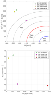 |
Fig. 11. Top panel: Toomroe diagram of the RAVE stars of this paper. Indicative limits for the thin and thick disc are plotted. Bottom panel: orbit energy vs. Lz plot of the stars. |
6. Summary of the properties of the four metal-poor RAVE stars
In this section we give a brief summary of the main properties of each of the four RAVE stars by combining all the information we obtained: chemistry, ages and masses, and kinematics.
6.1. 201359581 (S1)
This object is the only star of the sample where the temperature derived from the high-resolution spectrum is 380 K lower than the Teff derived from the lower resolution RAVE spectrum and the Teff derived from the IRFM. We already noticed in Valentini et al. (2017) that the IRFM tends to overestimate temperatures at Teff > 5000 K. This is probably because of the adoption of RAVE parameters as an input in the IRFM from RAVE-DR5. The miscalculated temperature from the RAVE spectrum led to a underestimated age for this star (see Appendix D). The Teff derived from high-resolution spectroscopy brings the age back into agreement with the expectation of this very metal-poor star being old. This is the star with the lower value of Δν and νmax, and, looking at its position in the HR diagram (Fig. 7) it is the only object that could be confused with a red clump star, which would then contribute to more uncertain estimates of mass and radius, and therefore age (mostly due to mass loss). The PDF of the age has a complex profile that is multi-peaked. Among the four stars, this is the object with the largest [C/Fe] ratio (around 0.30 dex). The star also has a high Ba and Eu and a [Eu/Ba] ratio of 0.3 ± 0.11. The small variation (few km s−1) in radial velocity and the big error (>5 km s−1) associated with Gaia radial velocity suggest that this object can be a binary star. Becuase of the flags in the astrometric solutions, the orbital parameters obtained for this star are larger, since we adopted the less precise proper motions from UCAC-5 catalogue (Zacharias et al. 2017). The star has an highly eccentric orbit and, looking at the Toomroe diagram in Fig. 11, it can be classified as a halo star.
6.2. 205997746 (S2)
The star 205997746 (S2) is not C-enhanced; it is below the RGB bump (see Fig. 7). The star appears enhanced in Na, where [Na/Fe] = +1.18 dex, but this result has to be taken carefully. This might be due to unresolved Na interstellar lines that hamper the abundance measurement. For this reason we are adopting this value as an upper limit. The star is alpha enhanced, and it is rich in Eu ([Eu/Fe] = 0.41) and it can be classified as an r-rich star ([Eu/Fe] > 0.3). The star is the richest in Cu (and poor C) of our sample. The age of this star presents a multi-peaked PDF, as is visible from Figs. 8 and E.2. Looking at the kinematics of the object, Fig. 11, the star seems a typical halo star.
6.3. 206034668 (S3)
Looking at the HR diagram in Fig. 7, the star 206034668 (S3) is located below the bump. This star is alpha-enhanced and it does not show C enhancement. This star is the richest star in Ba of our sample, while [Eu/Fe] is almost solar (r-poor). The low C abundance and the absence of vrad variation that might indicate binarity suggest that the star is not Ba-enriched via mass transfer from a more massive companion while in the AGB phase. If we use the element ratios as a diagnostic we find [Eu/Ba] = −0.89 ± 0.12 and [Sr/Ba] = −0.89 ± 0.15. Following (Spite et al. 2018, Fig. 4), these ratios put the star outside the correlation of [Eu/Ba] and [Ba/Fe], suggesting an origin from an environment with different chemical history than the Galactic Halo. When looking at mass and age of 201034668, PARAM provides different results depending on the seismic pipeline adopted. The COR seismic values provided a double-peaked age PDF, with no probability that the star is younger than 4 Gyr when GRD seismic values lead to older age. In all of the cases the age PDF extends beyond 30 Gyr or is truncated when the age prior is adopted (shown in Fig. E.2). The star seems to have a slightly retrograde orbit: in the Toomroe diagram the star is beyond the −220 km s−1; the slightly retrograde orbit is also maintained when integrating the orbit using Gaia DR2 distances. This star has an angular velocity of vϕmean = −0.133 km s−1 and it is on a highly energetic orbit, looking at the bottom panel of Fig. 11. The Ba and Eu enrichment, combined with the retrograde orbit, suggests that this star might be accreted from a system with larger Ba enrichment, such as a dSph galaxy (Spite et al. 2018).
6.4. 206443679 (S4)
The star 206443679 (S4) is well located below the RGB bump. The α enrichment, the high Eu content ([Eu/Fe] = 0.79 dex), and low C content suggest that the star is chemically a typical r-rich halo star. The star has also high Sr and Ba contents ([Ba/Fe] = 0.83 dex; [Sr/Fe] = 0.69 dex), giving [Sr/Ba] = −0.14. Following (Spite et al. 2018, Fig. 4), this puts the star very close to the pure r-process production limit. The star has an orbit typical of a thick disc star, however, its metallicity of [Fe/H] = −2.2 dex is indicative of a halo/accreted origin. This star could have acquired the presently observed orbit in two ways: First, keeping in mind its age of 9−10 Gyr, it could have belonged to the last massive merger of the Milky Way. Figure 1 of Helmi et al. (2018) shows that this region of the Toomre diagram is degenerate with respect to accreted and in situ born population. This requires an in-plane accretion, which can result from massive mergers being dragged into the disc mid-plane by dynamical friction (Read et al. 2009). Second, the inner halo has long been known to acquire angular momentum from the bar causing it to slow down, as seen in the N-body simulations (e.g. Athanassoula 2003; Minchev et al. 2012). With a guiding radius of 7 kpc, this star may have therefore gained rotational support from the bar.
7. Conclusions
As part of a pilot programme aimed at obtaining precise stellar parameters and ages for very metal-poor stars with available seismic information, we determined mass and ages for a sample of four RAVE metal-poor stars. We also characterised the stars by combining the information on age with their chemical profile (form high-resolution UVES spectra, covering different production channels) and their kinematics. Our analysis took advantage of the seismic information derived from K2 light curves (Campaigns 1 and 3): asteroseismology was first involved in the spectroscopic analysis and then in the mass and age determination using a Bayesian approach. We provided a full analysis (stellar parameters, chemistry and ages) using both intermediate-resolution spectra (RAVE; R = 7500) and high-resolution spectra (ESO-UVES; R = 110 000). We found abundances and atmospheric parameters derived from the high-resolution spectra to be in agreement with the atmospheric parameters derived from RAVE spectra once our strategy of making use of the seismic gravities and iterating on a more consistent (log(g), Teff) pair is adopted, as described in Valentini et al. (2017).
In addition we provide a comparison of log(g) derived using three different methods: (a) from the classical spectroscopic analysis, (b) from Gaia DR2 parallaxes (Eq. (1)), and (c) from asteroseismology (Eq. (3)). The three estimated values are in agreement within errors and seismic log(g) demonstrated to be reliable even at low metallicities and have the advantage of providing the most precise measurement. At low metallicities the classical log(g) derived via ionisation equilibrium is affected by NLTE effects, which may hamper the correct estimate of gravity and temperature. The log(g)ϖ, even if it has a large uncertainty due to the mass assumption, can be used as a good prior for spectroscopic analysis of red giant spectra, in particular of spectra with known Teff-log(g) degeneracies (as in RAVE) when no seismic information is available.
The more precise and self-consistent stellar parameters obtained for the four RAVE stars, when combined with Δν and νmax estimated from different seismic pipelines, deliver masses, and ages with 9% and 30−35% uncertainties, respectively. Ages for a field red giants of this precision opens new perspectives to the field of Galactic archaeology (see also, Miglio et al. 2017). Along this work we also investigated the impact of different assumptions on the above uncertainties. The main conclusions can be summarised as follows:
-
The impact of spectral resolution/short-wavelength interval: masses and ages were obtained from RAVE and UVES spectra using the same strategy of iterating on the best (log g, Teff) pair using the seismic gravity and IRFM temperatures as the priors. In the case of the RAVE spectra the known degeneracies lead to large uncertainties in mass and age. In one case, when the IRFM Teff was inaccurate by ∼250 K (i.e. outside the flexibility range in temperature during the iteration) an erroneous age determination occurs. However, in this case, the posteriors of temperature, mass, and age are in tension with those of Δν and νmax. This already tends to indicate an erroneous determination on one of the input parameters, and thus potentially leads to an erroneous age determination; this case is well illustrated by that specific example.
-
Impact of the different seismic pipelines: The adoption of different seismic pipelines has made clear the important impact the uncertainties on Δν and νmax estimates can have on the resulting masses and ages. However, also in this case, it is possible to select those seismic estimates that seem to be in better agreement with the quality of the light curves available, making sure that only the best seismic parameters are used. In this work we favoured the seismic method providing the lowest spread when compared to other methods (Pinsonneault et al. 2018, Fig. 10).
-
The impact of surface temperature scale: A shift of −100 K in Teff leads to a mass underestimation of ∼10% and, as a consequence, a stellar age that is older by ∼30%; if temperatures are overestimated the effect works in the opposite direction.
-
The impact of [α/Fe] ratios: In this case the impact is less important than those discussed above because they are only of a few percent in age. In the case of the RAVE spectra, where the [α/Fe] has larger uncertainties, we computed ages and masses for different [α/Fe] ratios and the effects were minor.
-
The impact of mass nloss: As pointed out in Anders et al. (2017) and Casagrande et al. (2016), the impact of mass loss becomes important in the red clump phase. Our stars are compatible with being RGB where the mass-loss impact is expected to be minor (as is also shown by the computation made in the present work).
-
The impact of an accretion event: The seismic age measurement relies on the fact that the age of a red giant is proportional to the time spent on the MS and therefore its mass. Any mass accretion event hampers this assumption (rejuvenating the star). Radial velocity variations (due to binarity) or chemical hints of mass transfer (mostly the contributions of C or s-process elements due to AGB-mass transfer) must raise a flag regarding the accuracy of the ages measured with asteroseismology. For three stars of our sample we do not find any clear sign of radial velocity variability nor any clear chemical signature of mass transfer from a companion, and therefore we consider our ages reliable.
This pilot project shows that it is possible to use asteroseismology for determining precise and consistent masses and ages of metal-poor field giants. Together with nucleo-cosmo-chronometry, seismology provides the only way to estimate the ages of distant field stars. However, this important new tool needs key steps to be followed, which are (i) a consistent spectroscopic analysis which delivers not only detailed abundances, but also a consistent (log(g); Teff) pair; (ii) a careful and critical use of the seismic inputs; and (iii) an analysis of the posterior distributions of all output parameters to look for tensions with the seismic input that might be indicative of erroneous parameter estimates. The use of seismic log(g) and a temperature prior in an iterative way (see Valentini et al. and references therein) is thus a critical step in the analysis. This important step assures that the atmospheric parameters used for deriving mass and age with asteroseismology is consistent with the seismic inputs used in the code, which also offers a new way to provide more reliable surface temperatures.
In the near future the impact of the Gaia data should become important thanks to a better understanding of the parallax offsets and also in terms of narrowing the current posterior age distributions (see Rodrigues et al. 2017, discussion). For now, Gaia DR2 data are already useful to better define the orbits of the studied stars.
Our strategy will enable a more serious programme towards determining ages for giant halo field stars, that is complementary to nucleo-cosmo-chronometry. However, our approach has the following two advantages: it applies to all stars and not necessarily only to stars that are strongly r-process enhanced, and it provides ages with smaller uncertainties. Detailed abundance measurements are also necessary to gauge possible effects of mass accretion, which would systematically shift the seismic ages. Finally, the results of this pilot programme pave the path for a more extensive study of metal-poor stars with asteroseismology, delivering samples with age estimates to a ∼30% precision, hence superior to all that is currently available for field metal-poor distant stars in terms of age determinations. It seems realistic to imagine that in the near future we will be able to add the age dimension in the chemical diagrams of the metal-poor universe (e.g. Cescutti & Chiappini 2014; Sakari et al. 2018; Spite et al. 2018), thus contributing enormously to our understanding of the first phases of the galaxy assembly and early nucleosynthesis.
Code available at: https://github.com/alexji/moog17scat
Available at the website http://nlte.mpia.de/
Codes available at https://github.com/casaluca/bolometric-corrections
Code available at http://github.com/jobovy/galpy
Acknowledgments
MV and CC acknowledge the DFG project number 283705981: “Analysing the chemical fingerprints left by the first stars: chemical abundances in the oldest stars”. DB is supported in the form of work contract FCT/MCTES through national funds and by FEDER through COMPETE2020 in connection to these grants: UID/FIS/04434/2019; PTDC/FIS-AST/30389/2017 & POCI-01-0145-FEDER-030389. AM, WJC, GRD, and YPE acknowledge the support of the UK Science and Technology Facilities Council (STFC). TSR acknowledges financial support from Premiale 2015 MITiC (PI B. Garilli). Authors MV, CC, DB acknowledge support from the “ChETEC” COST Action (CA16117), supported by COST (European Cooperation in Science and Technology). SM acknowledges support from NASA grant NNX15AF13G, NSF grant AST-1411685, and the Ramon y Cajal fellowship number RYC-2015-17697. The authors acknowledge the International Space Science Institute (ISSI-Bern), which hosted the first AsteroSTEP meetings (https://www.asterostep.eu). This work has made use of the VALD database, operated at Uppsala University, the Institute of Astronomy RAS in Moscow, and the University of Vienna. Based on data obtained from ESO-UVES instrument under proposal ID: 099.D-0913(A). Funding for RAVE has been provided by: the Australian Astronomical Observatory; the Leibniz-Institut fuer Astrophysik Potsdam (AIP); the Australian National University; the Australian Research Council; the French National Research Agency; the German Research Foundation (SPP 1177 and SFB 881); the European Research Council (ERC-StG 240271 Galactica); the Istituto Nazionale di Astrofisica at Padova; The Johns Hopkins University; the National Science Foundation of the USA (AST-0908326); the W. M. Keck foundation; the Macquarie University; the Netherlands Research School for Astronomy; the Natural Sciences and Engineering Research Council of Canada; the Slovenian Research Agency; the Swiss National Science Foundation; the Science & Technology Facilities Council of the UK; Opticon; Strasbourg Observatory; and the Universities of Groningen, Heidelberg and Sydney. The RAVE web site is at: https://www.rave-survey.org. This work has made use of data from the European Space Agency (ESA) mission Gaia (https://www.cosmos.esa.int/gaia), processed by the Gaia Data Processing and Analysis Consortium (DPAC, https://www.cosmos.esa.int/web/gaia/dpac/consortium). Funding for the DPAC has been provided by national institutions, in particular the institutions participating in the Gaia Multilateral Agreement. We finally acknowledge the anonymous referee for useful remarks.
References
- Abate, C., Pols, O. R., Izzard, R. G., & Karakas, A. I. 2015, A&A, 581, A22 [NASA ADS] [CrossRef] [EDP Sciences] [Google Scholar]
- Abolfathi, B., Aguado, D. S., Aguilar, G., et al. 2018, ApJS, 235, 42 [NASA ADS] [CrossRef] [Google Scholar]
- Anders, F., Chiappini, C., Rodrigues, T. S., et al. 2017, A&A, 597, A30 [NASA ADS] [CrossRef] [EDP Sciences] [Google Scholar]
- Asplund, M., Grevesse, N., Sauval, A. J., & Scott, P. 2009, ARA&A, 47, 481 [NASA ADS] [CrossRef] [Google Scholar]
- Athanassoula, E. 2003, MNRAS, 341, 1179 [NASA ADS] [CrossRef] [Google Scholar]
- Bailer-Jones, C. A. L., Rybizki, J., Fouesneau, M., Mantelet, G., & Andrae, R. 2018, AJ, 158, 58 [NASA ADS] [CrossRef] [Google Scholar]
- Beers, T. C., & Christlieb, N. 2005, ARA&A, 43, 531 [NASA ADS] [CrossRef] [Google Scholar]
- Bergemann, M. 2011, MNRAS, 413, 2184 [NASA ADS] [CrossRef] [Google Scholar]
- Bergemann, M., & Gehren, T. 2008, A&A, 492, 823 [NASA ADS] [CrossRef] [EDP Sciences] [Google Scholar]
- Bergemann, M., Lind, K., Collet, R., Magic, Z., & Asplund, M. 2012, MNRAS, 427, 27 [NASA ADS] [CrossRef] [Google Scholar]
- Boffin, H. M. J., Carraro, G., & Beccari, G. 2015, Ecology of Blue Straggler Stars (Springer) [Google Scholar]
- Borucki, W. J., Koch, D., Basri, G., et al. 2010, Science, 327, 977 [NASA ADS] [CrossRef] [PubMed] [Google Scholar]
- Bovy, J. 2015, ApJS, 216, 29 [NASA ADS] [CrossRef] [Google Scholar]
- Casagrande, L., & VandenBerg, D. A. 2014, MNRAS, 444, 392 [NASA ADS] [CrossRef] [MathSciNet] [Google Scholar]
- Casagrande, L., & VandenBerg, D. A. 2018, MNRAS, 475, 5023 [NASA ADS] [CrossRef] [Google Scholar]
- Casagrande, L., Silva Aguirre, V., Stello, D., et al. 2014, ApJ, 787, 110 [NASA ADS] [CrossRef] [Google Scholar]
- Casagrande, L., Silva Aguirre, V., Schlesinger, K. J., et al. 2016, MNRAS, 455, 987 [NASA ADS] [CrossRef] [Google Scholar]
- Casey, A. R., Hawkins, K., Hogg, D. W., et al. 2017, ApJ, 840, 59 [NASA ADS] [CrossRef] [Google Scholar]
- Casey, A. R., Kennedy, G. M., Hartle, T. R., & Schlaufman, K. C. 2018, MNRAS, 478, 2812 [NASA ADS] [CrossRef] [Google Scholar]
- Cayrel, R., Hill, V., Beers, T. C., et al. 2001, Nature, 409, 691 [NASA ADS] [CrossRef] [PubMed] [Google Scholar]
- Cescutti, G., & Chiappini, C. 2014, A&A, 565, A51 [NASA ADS] [CrossRef] [EDP Sciences] [Google Scholar]
- Chiappini, C. 2013, Astron. Nachr., 334, 595 [NASA ADS] [CrossRef] [Google Scholar]
- Christlieb, N., Beers, T. C., Barklem, P. S., et al. 2004, A&A, 428, 1027 [NASA ADS] [CrossRef] [EDP Sciences] [Google Scholar]
- Cowan, J. J., Sneden, C., Burles, S., et al. 2002, ApJ, 572, 861 [NASA ADS] [CrossRef] [Google Scholar]
- da Silva, L., Girardi, L., Pasquini, L., et al. 2006, A&A, 458, 609 [NASA ADS] [CrossRef] [EDP Sciences] [Google Scholar]
- Davies, G. R., & Miglio, A. 2016, Astron. Nachr., 337, 774 [NASA ADS] [CrossRef] [Google Scholar]
- Davies, G. R., Handberg, R., Miglio, A., et al. 2014, MNRAS, 445, L94 [NASA ADS] [CrossRef] [Google Scholar]
- Davies, G. R., Silva Aguirre, V., Bedding, T. R., et al. 2016, MNRAS, 456, 2183 [NASA ADS] [CrossRef] [Google Scholar]
- Dekker, H., D’Odorico, S., Kaufer, A., Delabre, B., & Kotzlowski, H. 2000, in Optical and IR Telescope Instrumentation and Detectors, eds. M. Iye, & A. F. Moorwood, Proc. SPIE, 4008, 534 [Google Scholar]
- De Ridder, J., Barban, C., Baudin, F., et al. 2009, Nature, 459, 398 [Google Scholar]
- Elsworth, Y., Hekker, S., Basu, S., & Davies, G. R. 2017, MNRAS, 466, 3344 [NASA ADS] [CrossRef] [Google Scholar]
- Epstein, C. R., Elsworth, Y. P., Johnson, J. A., et al. 2014, ApJ, 785, L28 [NASA ADS] [CrossRef] [Google Scholar]
- Feuillet, D. K., Bovy, J., Holtzman, J., et al. 2016, ApJ, 817, 40 [NASA ADS] [CrossRef] [Google Scholar]
- Frebel, A., & Norris, J. E. 2015, ARA&A, 53, 631 [NASA ADS] [CrossRef] [Google Scholar]
- Frebel, A., Christlieb, N., Norris, J. E., et al. 2007, ApJ, 660, L117 [NASA ADS] [CrossRef] [Google Scholar]
- Gaia Collaboration (Prusti, T., et al.) 2016, A&A, 595, A1 [NASA ADS] [CrossRef] [EDP Sciences] [Google Scholar]
- Gaia Collaboration (Brown, A. G. A., et al.) 2018, A&A, 616, A1 [NASA ADS] [CrossRef] [EDP Sciences] [Google Scholar]
- Green, G. M., Schlafly, E. F., Finkbeiner, D., et al. 2018, MNRAS, 478, 651 [NASA ADS] [CrossRef] [Google Scholar]
- Grevesse, N., & Noels, A. 1993, Phys. Scr. Vol. T, 47, 133 [NASA ADS] [CrossRef] [Google Scholar]
- Gustafsson, B., Edvardsson, B., Eriksson, K., et al. 2008, A&A, 486, 951 [NASA ADS] [CrossRef] [EDP Sciences] [Google Scholar]
- Hansen, B. M. S., Richer, H. B., Fahlman, G. G., et al. 2004, ApJS, 155, 551 [NASA ADS] [CrossRef] [Google Scholar]
- Hekker, S., Broomhall, A.-M., Chaplin, W. J., et al. 2010, MNRAS, 402, 2049 [NASA ADS] [CrossRef] [Google Scholar]
- Hekker, S., Elsworth, Y., Mosser, B., et al. 2012, A&A, 544, A90 [NASA ADS] [CrossRef] [EDP Sciences] [Google Scholar]
- Helmi, A., White, S. D. M., de Zeeuw, P. T., & Zhao, H. 1999, Nature, 402, 53 [NASA ADS] [CrossRef] [Google Scholar]
- Helmi, A., Babusiaux, C., Koppelman, H. H., et al. 2018, Nature, 563, 85 [NASA ADS] [CrossRef] [Google Scholar]
- Hill, V., Plez, B., Cayrel, R., et al. 2002, A&A, 387, 560 [NASA ADS] [CrossRef] [EDP Sciences] [Google Scholar]
- Hill, V., Christlieb, N., Beers, T. C., et al. 2017, A&A, 607, A91 [NASA ADS] [CrossRef] [EDP Sciences] [Google Scholar]
- Howell, S. B., Sobeck, C., Haas, M., et al. 2014, PASP, 126, 398 [NASA ADS] [CrossRef] [Google Scholar]
- Huber, D., Bedding, T. R., Stello, D., et al. 2011, ApJ, 743, 143 [NASA ADS] [CrossRef] [Google Scholar]
- Ivans, I. I., Simmerer, J., Sneden, C., et al. 2006, ApJ, 645, 613 [NASA ADS] [CrossRef] [Google Scholar]
- Jofré, P., & Weiss, A. 2011, A&A, 533, A59 [NASA ADS] [CrossRef] [EDP Sciences] [Google Scholar]
- Kalirai, J. S. 2012, Nature, 486, 90 [NASA ADS] [Google Scholar]
- Kallinger, T., De Ridder, J., Hekker, S., et al. 2014, A&A, 570, A41 [NASA ADS] [CrossRef] [EDP Sciences] [Google Scholar]
- Khan, S., Hall, O. J., Miglio, A., et al. 2018, ApJ, 859, 156 [NASA ADS] [CrossRef] [Google Scholar]
- Kilic, M., Bergeron, P., Dame, K., et al. 2019, MNRAS, 482, 965 [NASA ADS] [CrossRef] [Google Scholar]
- Kunder, A., Kordopatis, G., Steinmetz, M., et al. 2017, AJ, 153, 75 [NASA ADS] [CrossRef] [Google Scholar]
- Kupka, F., Piskunov, N., Ryabchikova, T. A., Stempels, H. C., & Weiss, W. W. 1999, A&AS, 138, 119 [NASA ADS] [CrossRef] [EDP Sciences] [MathSciNet] [PubMed] [Google Scholar]
- Kupka, F. G., Ryabchikova, T. A., Piskunov, N. E., Stempels, H. C., & Weiss, W. W. 2000, Balt. Astron., 9, 590 [NASA ADS] [Google Scholar]
- Lillo-Box, J., Barrado, D., Moya, A., et al. 2014, A&A, 562, A109 [NASA ADS] [CrossRef] [EDP Sciences] [Google Scholar]
- Lindegren, L., Hernandez, J., Bombrun, A., et al. 2018, A&A, 616, A2 [NASA ADS] [CrossRef] [EDP Sciences] [Google Scholar]
- Majewski, S. R., Schiavon, R. P., Frinchaboy, P. M., et al. 2017, AJ, 154, 94 [NASA ADS] [CrossRef] [Google Scholar]
- Masseron, T., Plez, B., Van Eck, S., et al. 2014, A&A, 571, A47 [NASA ADS] [CrossRef] [EDP Sciences] [Google Scholar]
- Mathur, S., García, R. A., Régulo, C., et al. 2010, A&A, 511, A46 [NASA ADS] [CrossRef] [EDP Sciences] [Google Scholar]
- Mathur, S., Hekker, S., Trampedach, R., et al. 2011, ApJ, 741, 119 [NASA ADS] [CrossRef] [Google Scholar]
- Matijevič, G., Chiappini, C., Grebel, E. K., et al. 2017, A&A, 603, A19 [NASA ADS] [CrossRef] [EDP Sciences] [Google Scholar]
- Miglio, A., Brogaard, K., Stello, D., et al. 2012, MNRAS, 419, 2077 [NASA ADS] [CrossRef] [Google Scholar]
- Miglio, A., Chiappini, C., Morel, T., et al. 2013, MNRAS, 429, 423 [NASA ADS] [CrossRef] [Google Scholar]
- Miglio, A., Chaplin, W. J., Brogaard, K., et al. 2016, MNRAS, 461, 760 [NASA ADS] [CrossRef] [Google Scholar]
- Miglio, A., Chiappini, C., Mosser, B., et al. 2017, Astron. Nachr., 338, 644 [NASA ADS] [CrossRef] [Google Scholar]
- Minchev, I., Famaey, B., Quillen, A. C., et al. 2012, A&A, 548, A126 [NASA ADS] [CrossRef] [EDP Sciences] [Google Scholar]
- Mosser, B., & Appourchaux, T. 2009, A&A, 508, 877 [NASA ADS] [CrossRef] [EDP Sciences] [Google Scholar]
- Mosser, B., Barban, C., Montalbán, J., et al. 2011, A&A, 532, A86 [NASA ADS] [CrossRef] [EDP Sciences] [Google Scholar]
- Paxton, B., Bildsten, L., Dotter, A., et al. 2011, ApJS, 192, 3 [Google Scholar]
- Pérez Hernández, F., García, R. A., Corsaro, E., Triana, S. A., & De Ridder, J. 2016, A&A, 591, A99 [NASA ADS] [CrossRef] [EDP Sciences] [Google Scholar]
- Pinsonneault, M. H., Elsworth, Y., Epstein, C., et al. 2014, ApJS, 215, 19 [NASA ADS] [CrossRef] [Google Scholar]
- Pinsonneault, M. H., Elsworth, Y. P., Tayar, J., et al. 2018, ApJS, 239, 32 [NASA ADS] [CrossRef] [Google Scholar]
- Piskunov, N. E., Kupka, F., Ryabchikova, T. A., Weiss, W. W., & Jeffery, C. S. 1995, A&AS, 112, 525 [NASA ADS] [Google Scholar]
- Placco, V. M., Holmbeck, E. M., Frebel, A., et al. 2017, ApJ, 844, 18 [NASA ADS] [CrossRef] [Google Scholar]
- Queiroz, A. B. A., Anders, F., Santiago, B. X., et al. 2018, MNRAS, 476, 2556 [NASA ADS] [CrossRef] [Google Scholar]
- Read, J. I., Mayer, L., Brooks, A. M., Governato, F., & Lake, G. 2009, MNRAS, 397, 44 [NASA ADS] [CrossRef] [Google Scholar]
- Reimers, D. 1975, Mem. Soc. Roy. Sci. Liege, 8, 369 [Google Scholar]
- Rodrigues, T. S., Bossini, D., Miglio, A., et al. 2017, MNRAS, 467, 1433 [NASA ADS] [Google Scholar]
- Roederer, I. U., Preston, G. W., Thompson, I. B., et al. 2014a, AJ, 147, 136 [NASA ADS] [CrossRef] [Google Scholar]
- Roederer, I. U., Jacobson, H. R., Thanathibodee, T., Frebel, A., & Toller, E. 2014b, ApJ, 797, 69 [NASA ADS] [CrossRef] [Google Scholar]
- Ryabchikova, T. A., Piskunov, N. E., Kupka, F., & Weiss, W. W. 1997, Balt. Astron., 6, 244 [NASA ADS] [Google Scholar]
- Ryabchikova, T., Piskunov, N., Kurucz, R. L., et al. 2015, Phys. Scr., 90, 054005 [NASA ADS] [CrossRef] [Google Scholar]
- Sakari, C. M., Placco, V. M., Farrell, E. M., et al. 2018, ApJ, 868, 110 [NASA ADS] [CrossRef] [Google Scholar]
- Salaris, M., Chieffi, A., & Straniero, O. 1993, ApJ, 414, 580 [NASA ADS] [CrossRef] [Google Scholar]
- Schlegel, D. J., Finkbeiner, D. P., & Davis, M. 1998, ApJ, 500, 525 [NASA ADS] [CrossRef] [Google Scholar]
- Sharma, S., Stello, D., Bland-Hawthorn, J., Huber, D., & Bedding, T. R. 2016, ApJ, 822, 15 [NASA ADS] [CrossRef] [Google Scholar]
- Silva Aguirre, V., Bojsen-Hansen, M., Slumstrup, D., et al. 2018, MNRAS, 475, 5487 [NASA ADS] [Google Scholar]
- Sneden, C., Cowan, J. J., Lawler, J. E., et al. 2003, ApJ, 591, 936 [NASA ADS] [CrossRef] [Google Scholar]
- Sobeck, J. S., Kraft, R. P., Sneden, C., et al. 2011, AJ, 141, 175 [NASA ADS] [CrossRef] [Google Scholar]
- Spite, F., Spite, M., Barbuy, B., et al. 2018, A&A, 611, A30 [NASA ADS] [CrossRef] [EDP Sciences] [Google Scholar]
- Steinmetz, M., Zwitter, T., Siebert, A., et al. 2006, AJ, 132, 1645 [NASA ADS] [CrossRef] [Google Scholar]
- Stello, D., Huber, D., Sharma, S., et al. 2015, ApJ, 809, L3 [NASA ADS] [CrossRef] [Google Scholar]
- Valentini, M., Morel, T., Miglio, A., Fossati, L., & Munari, U. 2013, Eur. Phys. J. Web Conf., 43, 03006 [CrossRef] [Google Scholar]
- Valentini, M., Chiappini, C., Davies, G. R., et al. 2017, A&A, 600, A66 [NASA ADS] [CrossRef] [EDP Sciences] [Google Scholar]
- van der Maaten, L., & Hinton, G. 2008, J. Mach. Learn. Res., 9, 85 [Google Scholar]
- Yu, J., Huber, D., Bedding, T. R., et al. 2018, ApJS, 236, 42 [NASA ADS] [CrossRef] [Google Scholar]
- Zacharias, N., Finch, C., & Frouard, J. 2017, VizieR Online Data Catalog: I/340 [Google Scholar]
- Zinn, J. C., Pinsonneault, M. H., Huber, D., & Stello, D. 2019, ApJ, 878, 136 [NASA ADS] [CrossRef] [Google Scholar]
Appendix A: Selection of Δν and νmax
For the four RAVE metal-poor stars analysed in the present work we obtained Δν and νmax from four different pipelines. We decided to select the best Δν and νmax pair by looking at the performances of the four pipelines for each object. When looking at the power spectrum (see Fig. A.1) it is visible that the uncertainty on the A2Z results is clearly too large in at least two instances. This is probably connected with the method and its sensitivity to poorly sampled data. For this reason we do not favour the A2Z results for the νmax.
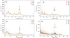 |
Fig. A.1. Normalised power spectrum of the RAVE stars (original: orange line; smoothed: blue). The νmax values from the different pipelines are plotted: GRD (green), COR (red), YE (purple), and A2Z (brown). |
For better understanding the Δν results, we created S/N spectra (Fig. A.2), and then analysed S/N spectra as a function of frequency mod Δν divided by Δν (one realisation per each pipeline). The same analysis was performed using Δν+eDnu. If the uncertainty is sensible (i.e. not too large) we might expect to see repeated structures. If eΔν is too large the repeated structure goes away.
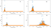 |
Fig. A.2. S/N spectra of the RAVE metal-poor stars of this work. |
This check led to the following conclusions regarding Δν:
-
201359581 (S1), nothing is clearly visible in both S/N realisations.
-
205997746 (S2) has a nice l = 0, 2 pair with all pipelines.
-
206034668 (S3) has no result from A2Z, but the other three pipelines all have results even if the epsilon value is not agreed on. We note that YE and GRD agree on epsilon. The sharpness of the peaks in this star seems to be better for GRD and YE rather than BM.
-
206443679 (S4) is easy to see the l = 0, 2 and plenty of other repeated structure. Every pipeline agrees for this star.
This is probably a result of the different method used and the degree to which the pipelines are set up to be conservative. With only four stars, we do not have the disadvantage of a large sample to manage, which has uncertainties that are too large. From the tests above we concluded that BM and GRD have the lowest and probably the most realistic uncertainties for these four stars; (his conclusion does not necessarily hold for other stars. We therefore move forward with the analysis using only the GRD and BM results. For future works we will keep considering results from different pipelines, performing this analysis for every target.
Δν and νmax as measured by the four different pipelines.
Appendix B: Analysis of UVES spectra
Chemical abundances derived for the metal-poor stars presented in this work.
Appendix C: Tests on α enhancement and Teff shifts
In the present work we use PARAM, which uses a set of MESA models that are not α-enhanced. The effect of the α-enhancement is taking into account by adopting the Salaris formula in Eq. (6). We tested this assumption using PARSEC models, for which α-enhanced computations are available. In Fig. C.1 we compare two sets of PARSEC tracks, covering MS to RGB tip phases. One set (plotted in red) is a set of tracks for 0.7, 1.0, and 1.3 M⊙ at [Fe/H] = −2.16 dex and [α/Fe] = 0.4 dex, a set of tracks at the corresponding metallicity [Fe/H] = −1.86 dex (following Eq. (6)). The maximum deviation between the two set of tracks reaches the maximum in the RGB phase. Since the difference is negligible with respect to the typical errors we have on age, we adopted the Salaris et al. (1993) correction in our computations.
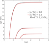 |
Fig. C.1. PARSEC tracks at [Fe/H] = −2.16 dex and [α/Fe] = 0.4 dex (in red) and PARSEC tracks at the corresponding metallicity [Fe/H] = −1.86, computed using Salaris formula (in black). Only MS-RGB tip is plotted and 3 masses are considered: 0.7, 1.0, and 1.3 M⊙. |
Appendix D: Masses and ages using RAVE atmospheric parameters and metallicities
We derived ages and masses for the four RAVE metal-poor stars using the atmospheric parameters derived from RAVE spectra using the seismic log(g). The RAVE spectra cover a small spectral range (8420−8780 Å) at intermediate resolution (R = 7500); element abundances may suffer from offsets and inaccuracies. For this reason we computed ages and masses for five different α enhancements. Two different mass-loss approximations (η = 0.2 and 0.4) have been considered and we adopted COR and GRD seismic parameters. Masses and ages derived using parameters measured from RAVE spectra are shown in Figs. D.1 (COR) and D.2 (GRD). The impact of temperature shift on this set of data has been tested by varying the Teff of ±100 K (see Fig. D.3) using COR seismic parameters. From Figs. D.1–D.3 it is possible to see the effect of the different α enhancements and mass-loss assumptions, and the effects of shifts in Teff.
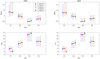 |
Fig. D.1. Mass and ages of the 5 stars determined using different [α/Fe] (0.0, 0.1, 0.2, 0.3, 0.4 dex, respectively) and 2 different η parameters (0.2 and 0.4) for mass loss. The COR seismic parameters and spectroscopic parameters derived from RAVE spectra and asteroseismology. |
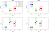 |
Fig. D.2. Mass and ages of the 5 stars, determined using different [α/Fe] (0.0, 0.1, 0.2, 0.3, 0.4 dex respectively) and 2 different η parameters (0.2 and 0.4) for mass loss. The GRD seismic parameters and spectroscopic parameters derived from RAVE spectra and asteroseismology. |
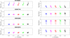 |
Fig. D.3. Mass and ages of the 5 stars determined using different [α/Fe] (0.0, 0.1, 0.2, 0.3, 0.4 dex in blue, magenta, red, green, and black, respectively) and varying the Teff of ±100 K in each α assumption (upward triangle for temperature increased, downward triangle for decreased). The BM_N (COR with new errors) seismic parameters and spectroscopic parameters derived from RAVE spectra and asteroseismology. |
Appendix E: PARAM tensions and additional results
S1 is an exemplary case of how an erroneus temperature determination leads to misleading age and mass values using PARAM. In the case of RAVE spectra the spectroscopically determined Teff is 300 K higher than the temperature derived from the high-resolution spectrum. However, as visible in Fig. E.1, the erroneus Teff lead to tensions between the a posteriori and input values of Δν, νmax, and Teff and to asymmetric PDFs. This does not happen when adopting the atmospheric parameters coming from high-resolution spectroscopy.
Ages and masses of the four RAVE stars as derived by PARAM, using COR seismic pipeline and stellar parameters obtained from different spectra, RAVE, and ESO-UVES (after adopting the strategy of using seismic gravities to find a more self-consistent surface temperature).
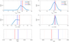 |
Fig. E.1. Left column: a posteriori Δν, νmax, and Teff of S1 using RAVE atmospheric parameters. The PDFs for Δν and νmax are shown as well. Right column: a posteriori Δν (and its PDF), νmax (and its PDF), and Teff of S1 using atmospheric parameters derived from UVES spectrum. |
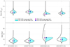 |
Fig. E.2. Violin plot of the PDFs of mass (top) and age (bottom) with input seismic parameters given by the COR pipeline with and without upper age limit (cyan and white shades, respectively). The mode of each pdf, with the errorbar representing the lower and upper 68th percentile of the PDF, is also indicated. |
Appendix F: M4 PARAM results in detail
The globular cluster M4 is the ideal testing ground for investigating the accuracy of our stellar age and mass determination with respect to other classic techniques. The cluster had been well investigated in the literature, and its age has been determined using both colour-magnitude diagram (CMD) fitting (e.g. Miglio et al. 2016) and the white dwarfs cooling sequence (Hansen et al. 2004): both techniques agree on an age of ∼13 Gyr with an error of 0.7 Gyr. The work of Miglio et al. (2016) also determined a typical mass of the stars in the RGB; i.e., MRGB = 0.84 M⊙ with an error of 0.05 M⊙.
In Fig. F.1 we report the individual mass and ages PDFs as determined using PARAM and we compare these with the literature results for M4. Our values are in a very good agreement with literature values with the exception of star M4−S4, which is a probable red clump star.
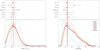 |
Fig. F.1. Masses (left column) and ages (right column) of the red giants in M4 analysed in this work. The thick red vertical line identifies the literature value, while the fine lines identify the upper and lower values. On the top row individual masses (left) and ages (right) are reported, where the errorbar indicates the 68th percentile of the PDF. At the bottom the individual PDFs for mass and ages are plotted. |
All Tables
Gaia DR2 data and seismic data for the 4 RAVE metal-poor stars studied in this work.
Radial velocity, atmospheric parameters, and abundances of the metal-poor RAVE stars in K2 Campaigns 1 and 3, as derived from RAVE spectra.
Atmospheric parameters and radial velocities of the stars as obtained from Gaia DR2 and from high-resolution UVES spectra.
Seismic mass and radius calculated using scaling relations (Teff measured from UVES spectra), and mass, radius, and age derived using PARAM, for the 4 metal-poor RAVE stars in K2 Campaigns 1 and 3.
Seismic distances and luminosities calculated using scaling relations, PARAM, distances obtained from Gaia parallaxes (both using the classical 1/ϖ and Bailer-Jones et al. 2018), distance calculated using StarHorse (Queiroz et al. 2018), and luminosity provided by Gaia DR2.
Input atmospheric parameters for the Epstein et al. (2014) stars and PARAM results of mass and age.
Input atmospheric parameters for the stars analysed in the M4 globular cluster Miglio et al. (2016) adopted in PARAM and resulting mass and age.
Reddening values for each stars as calculated from Schlegel et al. (1998), PARAM, and COR seismic values, StarHorse Queiroz et al. (2018) (spectroscopic atmospheric parameters and Gaia parallaxes) and Green et al. (2018).
Adopted proper motions for the orbit integration, plus orbit parameters of the stars in this work.
Ages and masses of the four RAVE stars as derived by PARAM, using COR seismic pipeline and stellar parameters obtained from different spectra, RAVE, and ESO-UVES (after adopting the strategy of using seismic gravities to find a more self-consistent surface temperature).
All Figures
|
Fig. 1. Spectra taken by the RAVE survey of the 4 metal-poor stars presented in this paper. Spectra are normalised and corrected for radial velocity; the Fe content labelled comes from the analysis of RAVE spectra using the same method as in Valentini et al. (2017). |
| In the text | |
|
Fig. 2. t-SNE projection of ∼420 000 RAVE spectra. The scaling in both direction is arbitrary, therefore the units on the axes are omitted. The colour scale corresponds to the gravity of the stars as computed by Kunder et al. (2017). Giants are shown in red and dwarfs in blue. Lighter shaded hexagons include fewer stars than darker ones. Over-plotted black dots indicate locations of RAVE stars in K2 Campaigns 1,3. Illustrated as stars are the RAVE-K2 objects studied in the present work, which fall in the metal-poor locus of the diagram. |
| In the text | |
|
Fig. 3. Δν and νmax as measured by different pipelines. Each colour (blue, magenta, red, and green) corresponds to a different pipeline (COR, GRD, A2Z, and YE; see appendix). The values plotted in black correspond to a further test using COR with inflated uncertainties (BM_N). |
| In the text | |
|
Fig. 4. Δν and νmax distribution of the 4 stars studied in this work. The Δν-νmax distribution distribution of the APOKASC sample is colour coded following the mass. |
| In the text | |
|
Fig. 5. Chemical abundance pattern [X/Fe] for the four metal-poor stars studied in this work. As a reference, the abundances pattern of the r-process enriched star CS 31082−001 are plotted as a dark grey line (abundances from Roederer et al. 2014b). |
| In the text | |
|
Fig. 6. Atmospheric parameters of the sample of metal-poor stars, as taken from literature and this work: RAVE spectra and seismic parameters (red squares), RAVE-DR5 (blue triangles), RAVE-on (cyan triangles), and ESO high-resolution spectra and seismic parameters (black circles). |
| In the text | |
|
Fig. 7. Top panel: position in the temperature – luminosity diagram of the 4 RAVE stars of this work (nomenclature following Table 1). Evolutionary tracks at masses M = 0.8 and 1.0 M⊙, at two different metallicities (Z = 0.00060 and 0.00197) are plotted. Middle panel: position in the temperature – νmax diagram of the four RAVE stars of this work, same tracks as top panel. Bottom panel: position in the temperature – Δν diagram of the four RAVE stars of this work, same tracks as top panel. Error bars of the plotted quantities are of the size of the points. |
| In the text | |
|
Fig. 8. Left column: violin plot of the PDFs of mass (top) and age (bottom). The right magenta shaded PDF is derived using the parameters from BM_N seismic set of parameters; the new errors take into account dispersion between pipelines and the PDFs on the left of the violin are calculated using seismic parameters from COR pipeline (black line, grey shaded) and varying the Teff of +100 K (dashed blue line) or −100 K (dotted red line). Right column: modes and 68 percentile errorbar of masses (top) and ages (bottom) of the 4 stars of this work. Magenta points indicate values computed using BM_N seismic values, black diamonds indicate the values derived using COR seismic values, and red and blue triangles indicate values obtained using COR seismic values and varying the Teff of −100 and +100 K, respectively. |
| In the text | |
|
Fig. 9. Mass and age comparison for the 9 stars presented in Epstein et al. (2014; blue diamonds) with the values derived in this work (red circles), in Pinsonneault et al. (2018; green triangles) and Yu et al. (2018; magenta triangles). Stars are indexed as in Table 8. |
| In the text | |
|
Fig. 10. Mass and ages of RGB stars in the metal-poor regime for a) four metal-poor RAVE stars with K2 seismic oscillations presented in this work (red diamonds); b) nine APOKASC the objects from Epstein et al. (2014) (original values as empty black circles; our new determination using PARAM and APOGEE-DR14 atmospheric parameters and abundances are shown as filled red circles), and c) seven stars in M4 from Miglio et al. (2016) recomputed with PARAM in this work (yellow triangles). |
| In the text | |
|
Fig. 11. Top panel: Toomroe diagram of the RAVE stars of this paper. Indicative limits for the thin and thick disc are plotted. Bottom panel: orbit energy vs. Lz plot of the stars. |
| In the text | |
|
Fig. A.1. Normalised power spectrum of the RAVE stars (original: orange line; smoothed: blue). The νmax values from the different pipelines are plotted: GRD (green), COR (red), YE (purple), and A2Z (brown). |
| In the text | |
|
Fig. A.2. S/N spectra of the RAVE metal-poor stars of this work. |
| In the text | |
|
Fig. C.1. PARSEC tracks at [Fe/H] = −2.16 dex and [α/Fe] = 0.4 dex (in red) and PARSEC tracks at the corresponding metallicity [Fe/H] = −1.86, computed using Salaris formula (in black). Only MS-RGB tip is plotted and 3 masses are considered: 0.7, 1.0, and 1.3 M⊙. |
| In the text | |
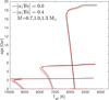 |
Fig. C.2. Same PARSEC tracks of Fig. C.1 but with temperature on the abscissa. |
| In the text | |
|
Fig. D.1. Mass and ages of the 5 stars determined using different [α/Fe] (0.0, 0.1, 0.2, 0.3, 0.4 dex, respectively) and 2 different η parameters (0.2 and 0.4) for mass loss. The COR seismic parameters and spectroscopic parameters derived from RAVE spectra and asteroseismology. |
| In the text | |
|
Fig. D.2. Mass and ages of the 5 stars, determined using different [α/Fe] (0.0, 0.1, 0.2, 0.3, 0.4 dex respectively) and 2 different η parameters (0.2 and 0.4) for mass loss. The GRD seismic parameters and spectroscopic parameters derived from RAVE spectra and asteroseismology. |
| In the text | |
|
Fig. D.3. Mass and ages of the 5 stars determined using different [α/Fe] (0.0, 0.1, 0.2, 0.3, 0.4 dex in blue, magenta, red, green, and black, respectively) and varying the Teff of ±100 K in each α assumption (upward triangle for temperature increased, downward triangle for decreased). The BM_N (COR with new errors) seismic parameters and spectroscopic parameters derived from RAVE spectra and asteroseismology. |
| In the text | |
|
Fig. E.1. Left column: a posteriori Δν, νmax, and Teff of S1 using RAVE atmospheric parameters. The PDFs for Δν and νmax are shown as well. Right column: a posteriori Δν (and its PDF), νmax (and its PDF), and Teff of S1 using atmospheric parameters derived from UVES spectrum. |
| In the text | |
|
Fig. E.2. Violin plot of the PDFs of mass (top) and age (bottom) with input seismic parameters given by the COR pipeline with and without upper age limit (cyan and white shades, respectively). The mode of each pdf, with the errorbar representing the lower and upper 68th percentile of the PDF, is also indicated. |
| In the text | |
|
Fig. F.1. Masses (left column) and ages (right column) of the red giants in M4 analysed in this work. The thick red vertical line identifies the literature value, while the fine lines identify the upper and lower values. On the top row individual masses (left) and ages (right) are reported, where the errorbar indicates the 68th percentile of the PDF. At the bottom the individual PDFs for mass and ages are plotted. |
| In the text | |
Current usage metrics show cumulative count of Article Views (full-text article views including HTML views, PDF and ePub downloads, according to the available data) and Abstracts Views on Vision4Press platform.
Data correspond to usage on the plateform after 2015. The current usage metrics is available 48-96 hours after online publication and is updated daily on week days.
Initial download of the metrics may take a while.