© ESO 2016

1. Introduction

The emission from the X-ray binary LS I + 61°303 has been observed from radio wavelengths to γ-rays (Taylor & Gregory 1982; Paredes et al. 1994; Mendelson & Mazeh 1989; Zamanov et al. 1999; Harrison et al. 2000; Abdo et al. 2009). Different variability patterns present in the observed flux at different energies constitute both a tool and a challenge for every possible interpretation of the physical processes behind the emission from this source. In this binary system, the compact object (neutron star or black hole) travels around a fast rotating Be star (see sketch in Fig. 1). Casares et al. (2005), who used only He I and He II lines in the spectral range 3850−5020 Å to avoid contamination from the emission lines of the decretion disk of the Be star, determined the phase of periastron as Φ = 0.23 ± 0.02 and an eccentricity of e = 0.72 ± 0.15.

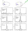Fig. 1 Top: sketch of the stellar system LS I + 61°303. We assume two ejections of relativistic electrons along the orbit as in Bosch-Ramon et al. (2006). The two ejections refill the conical precessing jet defined in Massi & Torricelli-Ciamponi (2014). The electrons emit by synchrotron and IC processes. The resulting jet parameters are given in Table 2. The ejection at periastron gives rise to gamma-ray emission only and the periodogram of this emission only shows P1, the orbital period. The ejection towards apastron is associated with gamma-ray and radio emission. The periodograms for both emissions show two features, at P1 and P2, the precession period of the jet. a) Lomb-Scargle periodogram for Fermi-LAT data from the orbital phase interval Φ = 0.0−0.5 (periastron). The orbital period P1 is clearly detected. b) Lomb-Scargle periodogram of the model gamma-ray data (IC) from the orbital phase interval Φ = 0.0−0.5 (periastron). The orbital period P1 is the only peak, in agreement with the observations. c) In the orbital phase interval Φ = 0.5−1.0 (apastron), there is a peak at the precession period P2 in addition to the orbital period P1. d) The two peaks at P1 and P2 in the apastron data are reproduced by the model. e) Lomb-Scargle periodogram for OVRO radio data for the whole orbital phase interval. Both P1 and P2 are present. f) Lomb-Scargle periodogram of the model radio data (synchrotron emission). Both peaks are reproduced by the model.

The specific nature of the interaction between the matter expelled from the Be star and the compact object defines the origin and physics of the observed emission; different models have been proposed assuming that either the compact object is accreting (Taylor et al. 1992; Marti & Paredes 1995; Bosch-Ramon et al. 2006; Romero et al. 2007; Massi & Torricelli-Ciamponi 2014) or non-accreting (Maraschi et al. 1981; Chernyakova et al. 2006; Dubus 2006). The challenge of all models is their capability of reproducing both the observed emission over the entire spectrum and the temporal variability specific of each energy range. In fact, the observed periodicities in different energy bands constitute a useful test for the validity of each model and provide the opportunity to allow the determination of the emission origin in LS I + 61°303.

Massi & Torricelli-Ciamponi (2014) have developed a model that fits the observed radio emission from LS I + 61°303 and its periodicities. In this model the radio emission is due to a precessing (P₂) jet that is periodically (P₁) refilled with relativistic particles. In this paper we further test our model by extending its capabilities to reproduce the GeV gamma-ray emission as well. The emission, for both radio and gamma-ray energy bands, is produced by energetic particles ejected twice along the orbit of LS I + 61°303, as in the context of accretion models.

The Bondi & Hoyle (1944) accretion rate $\mathit{Ṁ}\mathrm{\propto }\frac{\mathit{\rho }}{{\mathit{v}}^{\mathrm{3}}}$ onto a compact object, in addition to a main peak around periastron (where the density ρ has its maximum), already starts to develop a second accretion peak towards apastron for an eccentricity of e = 0.4 (Taylor et al. 1992). The reason for the second accretion peak towards apastron is the lower relative velocity v between the accretor and the Be star wind, which compensates for the lower density of the wind (Taylor et al. 1992; Marti & Paredes 1995; Bosch-Ramon et al. 2006; Romero et al. 2007). Indeed, gamma-ray emission in the GeV regime, observed by the Fermi Large Area Telescope (LAT), occurs both towards periastron and apastron. Radio outbursts, however, occur only towards apastron. These radio outbursts are affected by a long-term modulation (timescale years; Gregory 2002) and timing analysis results in two strong spectral features, P₁ and P₂, both of the order of one month (Massi & Jaron 2013; Massi et al. 2015; Massi & Torricelli-Ciamponi 2016). Concerning the GeV gamma-ray emission, timing analysis reveals that whereas the apastron emission is modulated by P₁ and P₂, identical to the radio emission, the periastron GeV emission is only modulated by P₁ (Jaron & Massi 2014). Ackermann et al. (2013) find that the GeV emission at apastron is affected by the long-term modulation (as the radio emission), while the periastron emission is not.

The aim of this paper is to investigate the physical processes responsible for the radio and gamma-ray emission and to explain the absence of P₂ in the emission at high energy around periastron as well as the lack of a periastron radio outburst. In Sect. 2, we report on the observational results revealing the nature of the physical processes behind the two periodicities P₁ and P₂. The model is described in Sect. 3 as a conical jet, precessing with period P₂, periodically (P₁) refilled with relativistic electrons twice along the orbit, and embedded in the photon field of the companion star. The emission of the electrons is due to synchrotron and inverse Compton (IC) processes. We compare the model with a more than five-year overlapping monitoring of gamma-ray and radio emission, by Fermi-LAT and the Owens Valley Radio Observatory (OVRO), whose calibration and reduction are presented in Sect. 4. In Sect. 5 we present our results and in Sect. 6 we give our conclusions.

2. The scenarios for LS I +61°303 and its periodicities

In this section we report on observational evidence for a precessing (P₂) jet (Sects. 2.1 and 2.2) and for two periodic (P₁) ejections along the orbit of LS I + 61°303 (Sect. 2.3).

2.1. The precessing (P₂) jet

Interferometric images of LS I + 61°303 at high resolution have at some epochs shown a one-sided jet structure and at other epochs a two-sided structure (Massi et al. 1993, 2002, 2004; Taylor et al. 2000). Dubus (2006) developed a numerical model for a pulsar nebula in which shocked material, due to the interaction of the relativistic pulsar wind with the stellar wind from the companion (Maraschi et al. 1981; Chernyakova et al. 2006), flows away in a comet-shape tail, i.e. compatible with a one-sided structure. Dhawan et al. (2006) performed a set of VLBA observations and related the observed varying morphology of the images to the rapid changes of a cometary tail. The same VLBA data, re-processed in Massi et al. (2012), confirm rapid changes in position angle and that the radio structure is at some epochs two-sided and at other epochs one-sided as expected from a jet of a microquasar with variable ejection angle (Massi et al. 2004). The compact jet associated with microquasars has a flat or even inverted radio spectrum (Fender et al. 1999). A flat or inverted radio spectrum for LS I + 61°303 was already proven in the past (Gregory et al. 1979; Massi & Kaufman Bernadó 2009) and was recently measured over the entire cm radio band (up to 9 mm) by Zimmermann et al. (2015).

As stated above, in the context of microquasars the changing position angle of the jet for LS I + 61°303 is attributed to a variation of the angle η between the jet and line of sight (Massi et al. 2004; Massi & Kaufman Bernadó 2009). Such a change gives rise to a continuously changing Doppler factor (the Doppler factor depending on the angle η) and therefore to a changing morphology. For small angles the counter-jet gets strongly attenuated and only the boosted approaching jet appears, giving rise to the microblazar one-sided morphology of LS I + 61°303 (Massi et al. 2013; Massi & Torricelli-Ciamponi 2014).

Is the variation of the ejection angle random or is there a periodicity? The motion of a jet can be revealed by the path traced by its core in consecutive images. The astrometry result in Massi et al. (2012) is that the core describes a periodic path with a precession period of 27−28 days (Massi et al. 2012). This determination has been confirmed by the timing analysis of 36.8 yr of radio data (Massi & Torricelli-Ciamponi 2016, and references therein). The results of the timing analysis are two dominant features at P₁ = 26.496 ± 0.013 d (the orbital period) and P₂ = 26.935 ± 0.013 d, and the period P₂ is clearly fully consistent with the period of 27−28 days that was determined by VLBA astrometry.

2.2. Beating between orbit (P₁) and precession (P₂)

The timing analysis by Massi & Torricelli-Ciamponi (2016) shows, as a minor feature with respect to P₁ and P₂, the long-term period P_long = 1628 ± 48 d. The same feature appears as well in the timing analysis of model data of a precessing (P₂) conical jet refilled periodically (with P₁) with relativistic electrons (Figs. 4a and b in Massi & Torricelli-Ciamponi 2016). Since P_long was not given as input in the model, this implies that P_long is the result of P₁ and P₂. In fact, the beating of ν₁ (1/P₁) and ν₂ (1/P₂) gives rise to a modulation with period 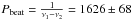${\mathit{P}}_{\mathrm{beat}}\mathrm{=}\frac{\mathrm{1}}{{\mathit{\nu }}_{\mathrm{1}}\mathrm{-}{\mathit{\nu }}_{\mathrm{2}}}\mathrm{=}\mathrm{1626}\mathrm{\pm }\mathrm{68}$ d, i.e. the long-term modulation.

Along with the identity of P_long with P_beat, an additional important point is that neither ν₁ nor ν₂ but rather their average, ${\mathit{P}}_{\mathrm{average}}\mathrm{=}\frac{\mathrm{2}}{{\mathit{\nu }}_{\mathrm{1}}\mathrm{+}{\mathit{\nu }}_{\mathrm{2}}}$, is modulated in a beating. The average of P₁ = 26.496 ± 0.013 d and P₂ = 26.935 ± 0.013 d is 26.71 d, and indeed the observed periodicity of the radio outbursts in LS I + 61°303, is 26.704 ± 0.004 d (Ray et al. 1997; Massi & Jaron 2013; Jaron & Massi 2013).

The fact that the periodicity of the outburst is P_average explains the well-known problem of the orbital shift of the outburst or timing residuals problem (Paredes et al. 1990; Gregory et al. 1999, and references therein). Orbital shifts or timing residuals occur because the outburst does not have orbital periodicity, i.e. P₁, but is in fact periodic with P_average. Massi & Jaron (2013) have shown mathematically that the timing residuals correspond to the difference between P₁ and P_average. When the outbursts are correctly folded with P_average, they cluster perfectly without any shift (Fig. 1 in Massi & Torricelli-Ciamponi 2016).

Direct determination of P₁ and P₂ in timing analysis or the determination of long-term modulation and orbital shift of data folded with P₁ are, therefore, equivalent indicators that the intensity variations are induced by the precessing jet. The first method finds the two physical periods directly, and the second method deals with the result of the beating. In addition to radio data, the periods P₁ and P₂ were also directly determined in the Lomb-Scargle spectrum of data at apastron for Fermi-LAT data (Jaron & Massi 2014) and X-ray data (D’Aì et al. 2016), whereas the long-term modulation (Zamanov et al. 2013) and orbital shift (Paredes-Fortuny et al. 2015) were found in the equivalent width EW of the Hα emission line.

2.3. The disk of the Be star

Before the discovery of the beating between P₁ and P₂, the assumptions for the long-term modulation were variations of the Be wind (Gregory & Neish 2002) with the further constraint of Be wind long-term variations influencing only the apastron and not the whole orbit because long-term variations in the emission only occur towards apastron (Ackermann et al. 2013). Whereas in the previous section we have seen the evidence for beating, in this section we report on observations probing the stability over the last 36.8 yr of the Be disk.

Cycles in varying Be stars change in length and disappear after 2−3 cycles, following the well-studied case of the binary system ζ Tau (Štefl et al. 2009, and references therein). In this context, radio variations induced by variations in the Be disk are predicted to be rather unstable. A powerful method for studying the stability of a periodic signal over time is its autocorrelation. If a period is stable the correlation coefficient should appear as an oscillatory sequence with peaks at multiples of that period. The analyses of 36.8 yr of radio data (Massi & Torricelli-Ciamponi 2016), corresponding to eight cycles of the long-term modulation, have definitely shown a very stable pattern for the radio data. The correlation coefficient of the observations shows a regular oscillation at P = 1626 d (their Fig. 5) as does the correlation coefficient of the model data of a precessing jet.

A stable P_long is what is expected for a beating of periods P₁ (orbital period) and P₂ (precession) without significant variations during the eight examined cycles (Massi & Torricelli-Ciamponi 2016). A stability in P₁ implies the same physical conditions in the accretion. This means that the decretion disk of the Be star was stable during the last 36.8 yr. This is consistent with the behaviour of Be stars. Over the last 100 yr, the Be star ζ Tau, whose emission has never disappeared completely, has gone through active stages, characterized by pronounced long-term variations, and quiet stages (Harmanec 1984). For a period of 30 yr, from 1920 to about 1950, there were no variations.

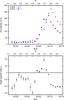Fig. 2 Top: radio light curve at 2 (red circles) and 8 GHz (blue squares) observed by the GBI from MJD 50 154.6 until 50 175.7 (orbital phase Φ = 0.1−1.0), averaged over one day. Bottom: radio spectral index α of the radio fluxes shown in the top panel clearly follows a two-peaked trend. One peak is during the large apastron radio outburst, which features a flat or inverted (α ≥ 0) spectrum during its rise. The other peak of the spectral index occurs at Φ = 0.25, i.e. at periastron, revealing that the spectrum becomes flattish (α ≈ 0) during this orbital phase as well (Massi & Kaufman Bernadó 2009).

The implications for the accretion along the orbit of LS I + 61°303 is that once the Be wind parameters such as as density and velocity (see Sect. 1) are relatively stable, the two accretion peaks from the compact object should always occur at the same two orbital phases. Is there any evidence for these predicted peaks at P₁? Fermi-LAT data over the large interval of 7.6 yr, when folded on the orbital period (Fig. 7) hint at two peaks. Indeed, timing analysis of this data results in a periodicity P₁ at periastron (Fig. 1a) and towards apastron (Fig. 1c), as already shown in Jaron & Massi (2014) with a smaller database. If the accretion peaks give rise to two ejections, then these two ejections, in the context of microquasars, should produce a flat spectrum twice along the orbit. Figure 2 shows the flux densities, S₁ and S₂, at two frequencies and their radio spectral index, $\mathit{\alpha }\mathrm{=}\frac{\log \mathrm{(}{\mathit{S}}_{\mathrm{1}}\mathit{/}{\mathit{S}}_{\mathrm{2}}\mathrm{)}}{\log \mathrm{(}{\mathit{\nu }}_{\mathrm{1}}\mathit{/}{\mathit{\nu }}_{\mathrm{2}}\mathrm{)}}$, along one orbital cycle. During the onset of the radio outburst α ≥ 0 as for microquasars, and attains a higher value at orbital phase 0.7 (i.e. apastron). In addition to that, around phase 0.2−0.3, i.e. at periastron, even if the flux density is very low, α shows a clear evolution, rises and reaches nearly zero at periastron, remains flattish, and then decays at the low value of −0.6. This trend of α is discussed for a radio database of years in Massi & Kaufman Bernadó (2009). As is shown in this paper, electrons suffer strong IC losses at periastron, the result of which is a short jet giving rise to a little flux. Nevertheless, the little flux does not lose its spectral property and the ratio of flux density at two frequencies (i.e. α) keeps the main characteristics as for the strong emission at apastron. Finally, optical observations by Mendelson & Mazeh (1989) showed two variations in orbital phase: one variation at periastron and another smaller variation at apastron. This optical emission could come from the hot accretion flow (optical synchrotron emission) as studies of X-ray binaries suggest (Poutanen & Veledina 2014).

3. Methods

In the following we extend the physical model of a precessing (P₂) jet periodically (P₁) refilled with relativistic electrons developed in Massi & Torricelli-Ciamponi (2014). Here the jet is refilled in two different parts of the orbit (Sect 3.1) and not only at apastron as in Massi & Torricelli-Ciamponi (2014). The synchrotron emission of such a jet is calculated as in Massi & Torricelli-Ciamponi (2014); in addition we calculate IC radiation here. Seed photons are stellar photons (external inverse Compton; EIC; Sect. 3.2) and the photons emitted by synchrotron radiation (synchrotron self Compton; SSC), i.e. jet photons (Sect. 3.3). The total IC emission from the model is calculated (Sect. 3.4). Electron energy losses are taken into account and the length of the jet is determined (in Sect. 3.5).

3.1. Relativistic electron distribution

Accretion theory predicts two maxima for the eccentric orbit of LS I + 61°303 (Taylor et al. 1992; Marti & Paredes 1995; Bosch-Ramon et al. 2006; Romero et al. 2007). One maximum is around periastron and the second is towards apastron. We indicate the two relativistic electron distributions as N_I (periastron) and N_II (towards apastron).

Quantities of this section include functions of the orbital phase Φ, or of the long-term modulation Θ, defined as 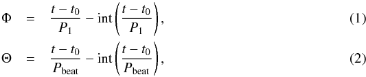$\begin{array}{ccc}\mathrm{\Phi }& \mathrm{=}& \frac{\mathit{t}\mathrm{-}{\mathit{t}}_{\mathrm{0}}}{{\mathit{P}}_{\mathrm{1}}}\mathrm{-}\mathrm{int}\left(\frac{\mathit{t}\mathrm{-}{\mathit{t}}_{\mathrm{0}}}{{\mathit{P}}_{\mathrm{1}}}\right)\mathit{,}\\ \mathrm{\Theta }& \mathrm{=}& \frac{\mathit{t}\mathrm{-}{\mathit{t}}_{\mathrm{0}}}{{\mathit{P}}_{\mathrm{beat}}}\mathrm{-}\mathrm{int}\left(\frac{\mathit{t}\mathrm{-}{\mathit{t}}_{\mathrm{0}}}{{\mathit{P}}_{\mathrm{beat}}}\right)\mathit{,}\end{array}$where t₀ = 43 366.275 MJD and int(x) takes the integer part of x.

In Massi & Torricelli-Ciamponi (2014), the radio emission was reproduced with a relativistic electron distribution N ejected around apastron which, once expressed in $\frac{\mathrm{electrons}}{\mathrm{c}{\mathrm{m}}^{\mathrm{3}}\mathrm{d}\mathit{\gamma }}$, is written as $\begin{array}{ccc}{\mathit{N}}_{\mathrm{II}}& \mathrm{=}{\mathit{K}}_{\mathrm{II}}\mathrm{\left(}\mathrm{\Phi }\mathrm{\right)}{\mathit{l}}^{\mathrm{-}{\mathit{a}}_{\mathrm{3}}}{\mathit{\gamma }}^{\mathrm{-}\mathit{p}}\mathit{,}& \end{array}$(3)with p = 1.8 and a₃ = 2(2 + p)/3 as derived by Kaiser (2006) for the adiabatic jet to take into account losses due to jet expansion.

In the present work we add another component to the above electron distribution, with a maximum around periastron, as follows: ${\mathit{N}}_{\mathrm{I}}\mathrm{=}{\mathit{K}}_{\mathrm{I}}\mathrm{\left(}\mathrm{\Phi }\mathrm{\right)}{\mathit{l}}^{\mathrm{-}{\mathit{a}}_{\mathrm{3}}}{\mathit{\gamma }}^{\mathrm{-}\mathit{p}}\mathit{.}$(4)This new electron component is injected and expands in the same conical magnetic structure defined by the model of Massi & Torricelli-Ciamponi (2014).

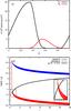Fig. 3 a) Orbital modulation of the electron density assumed in the model, as defined in Sect. 3.1. The two ejections are given at Φ = 0.35 and at Φ = 0.58. b) The maximum value of the Lorentz factor γ of the electrons as a function of the position l along the jet for the two ejections. The black curve is a plot of the minimum γ (Eq. (27)) necessary for the production of radio emission at 15 GHz for an initial magnetic field B0 = 5 G. The intersection point of the black curve with the red and blue lines defines the length of the jet at periastron and that of the jet towards apastron, respectively.

We assume that the accelerated electrons powered by accretion are injected both at periastron and apastron in similar ways and that the initial (i.e. at time t = t_min in l = 1) electron energy range is the same for the two distributions, ${\mathit{\gamma }}_{\mathrm{1}}\mathrm{\le }\mathit{\gamma }\mathrm{\left(}{\mathit{t}}_{\min }\mathrm{\right)}\mathrm{\le }{\mathit{\gamma }}_{\mathrm{2}}\mathit{.}$(5)However, as we see in Sect. 3.5, the value of γ evolves in a different way at periastron than at apastron owing to the different weight of radiative losses.

In our code each ejection of electrons is a sine function (of orbital phase) with different exponents (n, ex) for onset and decay. At each observing time the orbital phase and contribution of the sine functions for that phase are calculated. The results of the fit are position, amplitude, and exponents for both ejection functions (see Fig. 3 and Table 1).

For the specific case shown in Fig. 3, we computed the mean amount of energy injected per second in the form of relativistic electrons at the jet basis, l = 1. Taking a mean over the orbital phase of the electron density normalization factor, ${\mathit{K}}_{\mathrm{mean}}\mathrm{=}{{}^{\mathrm{\int }}}_{\mathrm{0}}^{\mathrm{1}}\mathrm{[}{\mathit{K}}_{\mathrm{I}}\mathrm{+}{\mathit{K}}_{\mathrm{II}}\mathrm{]}\mathrm{d\Phi }$, we obtain ${\mathit{L}}_{\mathrm{rel}}\mathrm{=}\mathrm{2}\mathrm{(}\mathit{\pi }{\mathit{r}}_{\mathrm{o}}^{\mathrm{2}}{\mathit{c}}^{\mathrm{)}}{\mathit{K}}_{\mathrm{mean}}{\mathrm{\left(}\mathit{m}{\mathit{c}}^{\mathrm{2}}\mathrm{\right)}}^{\mathrm{2}\mathrm{-}\mathit{p}}{\mathrm{\int }}_{{\mathit{\gamma }}_{\mathrm{1}}}^{{\mathit{\gamma }}_{\mathrm{2}}}{\mathit{\gamma }}^{\mathrm{1}\mathrm{-}\mathit{p}}\mathrm{d}\mathit{\gamma }\mathrm{\simeq }\mathrm{8}\mathrm{\times }{\mathrm{10}}^{\mathrm{35}}\mathrm{erg}\mathit{/}\mathrm{s}$(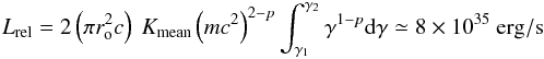6)for the two jets. Here r₀ = x₀tgξ is the initial jet radius and x₀ is a normalization length for the jet, which starts at x = x₀ and extends to x = x₀L with an opening angle ξ.

The orbital dependence of the injected energy follows the same modulation shown in Fig. 3 for the relativistic electron density with a maximum around Φ ~ 0.35 for which we have [L_rel] _MAX ≃ 1.8 × 10³⁶ erg/s.

3.2. Stellar seed photons

In order to take into account IC scattering of B0 star photons by relativistic electrons in the jet, it is necessary to compute the distance between the central B0 star and the generic position, x₀l, along the axis of the jet anchored to the orbiting compact object. With ψ being the opening angle of the precession cone, under the assumption that the jet precession axis is perpendicular to the orbital plane, we can compute

$\begin{array}{ccc}& & {\mathit{d}}_{\mathrm{\perp }}\mathrm{=}{\mathit{x}}_{\mathrm{0}}\mathit{l}\cos \mathit{\psi ,}\\ & & {\mathit{d}}_{\mathrm{plane}}\mathrm{=}\sqrt{\mathit{r}\mathrm{(}\mathrm{\Phi }{\mathrm{)}}^{\mathrm{2}}\mathrm{+}\mathrm{(}{\mathit{x}}_{\mathrm{0}}\mathit{l}\sin \mathit{\psi }{\mathrm{)}}^{\mathrm{2}}\mathrm{-}\mathrm{2}\mathit{r}\mathrm{\left(}{\mathit{x}}_{\mathrm{0}}\mathit{l}\sin \mathit{\psi }\mathrm{\right)}\cos \mathrm{\Omega }}\mathit{,}\\ & & {\mathit{d}}_{\mathrm{jet}\mathrm{-}\mathrm{star}}\mathrm{\left(}\mathit{l,}\mathrm{\Phi }\mathit{,}\mathrm{\Theta }\mathrm{\right)}\mathrm{=}\sqrt{{\mathit{d}}_{\mathrm{plane}}^{\mathrm{2}}\mathrm{+}{\mathit{d}}_{\mathrm{\perp }}^{\mathrm{2}}}\mathit{,}\end{array}$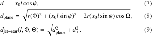where Ω (as in Massi & Torricelli-Ciamponi 2014) introduces the long-term modulation phase dependence and r(Φ) is the distance from the Be star to the point of the orbit corresponding to phase Φ. A sketch of the geometry is shown in Fig. 1.

Assuming for the star a blackbody emission with temperature T_∗, the photon density at the position x₀l, along the jet is ${\mathit{\rho }}_{\mathrm{star}}\mathrm{\left(}\mathit{l,}\mathrm{\Phi }\mathit{,}\mathrm{\Theta }\mathrm{\right)}\mathrm{=}\frac{\mathrm{4}\mathit{\pi }{\mathit{B}}_{\mathit{\nu }}\mathrm{\left(}{\mathit{T}}_{\mathrm{\ast }}\mathrm{\right)}}{\mathit{c}{\mathit{h}}^{\mathrm{2}}\mathit{\nu }}\frac{\mathit{\pi }{\mathit{R}}_{\mathrm{\ast }}^{\mathrm{2}}}{\mathrm{4}\mathit{\pi }{\mathit{d}}_{\mathrm{jet}\mathrm{-}\mathrm{star}}^{\mathrm{2}}}\mathrm{[}\mathrm{photons}\mathrm{c}{\mathrm{m}}^{-3}\mathrm{er}{\mathrm{g}}^{-1}\mathrm{]}\mathit{.}$(10)It is evident that this density value can only be affected by the different position along the orbit of the compact object, and hence of its associated jet, if the values of r(Φ) and x₀ are comparable. Hence, the orbital periodicity in the IC reprocessing of stellar photons show up only if relativistic electrons are present at distances from the orbital plane of the order of the ellipse’s semi-major axis, a, which in our case implies distances ≃7 × 10¹² cm (Massi et al. 2012). This fact implies that the jet scale dimensions, x₀, must be of this order of magnitude or even smaller.

The energy of IC reprocessed photons is linked to both electron and seed photon energies since the reprocessed photon energy, ϵ, fullfils the condition ϵ ~ γ²hν_seed. From the above Eq. (10) it is easy to derive that the maximum of the stellar photon number density is located at ν_peak such that hν_peak/kT_∗ ≃ 1.6. The photon density rapidly decreases for larger frequencies, while the decrease is slower for lower frequencies so that for hν/kT ≃ 0.1 the photon density is around 1/7 of its maximum value. Hence, in our case with T_∗ = 28 000 K, for ν_peak/ 16 ≤ ν_seed ≤ ν_peak, relativistic electrons with values of the Lorentz factor up to γ ~ 7 × 10⁴ can ensure that the reprocessed photons has energy of the order of 1 GeV, i.e. in the observational range chosen in this paper (see Sect. 4).

3.3. Jet seed photons

The jet photon density, owing to synchrotron emission inside the jet, can be computed as a function of the distance l along the jet axis, ${\mathit{\rho }}_{\mathrm{jet}}\mathrm{\left(}\mathit{l}\mathrm{\right)}\mathrm{=}\frac{\mathrm{4}\mathit{\pi }{\mathit{I}}_{\mathit{\nu }}\mathrm{\left(}\mathit{l}\mathrm{\right)}}{\mathit{c}{\mathit{h}}^{\mathrm{2}}\mathit{\nu }}\mathrm{[}\mathrm{photons}\hspace{0.17em}\mathrm{c}{\mathrm{m}}^{-3}\hspace{0.17em}\mathrm{er}{\mathrm{g}}^{-1}\mathrm{]}\mathit{.}$(11)In this expression, I_ν is the locally produced synchrotron emission in the optically thin limit 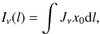${\mathit{I}}_{\mathit{\nu }}\mathrm{\left(}\mathit{l}\mathrm{\right)}\mathrm{=}\mathrm{\int }{\mathit{J}}_{\mathit{\nu }}{\mathit{x}}_{\mathrm{0}}\mathrm{d}\mathit{l,}$(12)and the notation is the same as in Massi & Torricelli-Ciamponi (2014). The above photon density is monotonically decreasing as ν^{− (p + 1)/2} with a maximum in the radio range where emission becomes optically thick.

Different energy ranges in synchrotron photon spectrum contribute to different energy ranges in the reprocessed SSC emission and the only condition we require is that reprocessed photons with energy in the 0.1−3 GeV band can be produced. Ginzburg & Syrovatski (1965) show that synchrotron emission is centred on a peak spectral frequency ν such that 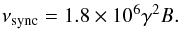${\mathit{\nu }}_{\mathrm{sync}}\mathrm{=}\mathrm{1.8}\mathrm{\times }{\mathrm{10}}^{\mathrm{6}}{\mathit{\gamma }}^{\mathrm{2}}\mathit{B}\mathit{.}$(13)Hence, our condition reads ${\mathit{\gamma }}^{\mathrm{2}}\mathit{h}{\mathit{\nu }}_{\mathrm{sync}}\mathrm{=}\mathrm{1.8}\mathrm{\times }{\mathrm{10}}^{\mathrm{6}}{\mathit{\gamma }}^{\mathrm{4}}\mathit{hB}\mathrm{~}\mathrm{1}\mathrm{GeV}\mathit{.}$(14)This condition is fulfilled if accelerated electrons exist with values of the Lorentz factor up to γ ~ 2 × 10⁴ with B₀ ~ 1 Gauss. This condition is not as strong as the previous condition found for stellar seed photons.

3.4. Inverse compton emission

In order to compare our theoretical model for GeV emission to available data we derive the quantity ${\mathit{F}}_{\mathrm{0.1}\mathrm{-}\mathrm{3}\hspace{0.17em}\mathrm{GeV}}\mathrm{=}\frac{\mathrm{1}}{\mathrm{4}\mathit{\pi }{\mathit{D}}^{\mathrm{2}}}\underset{\mathrm{0.1}\hspace{0.17em}\mathrm{GeV}}{\overset{\mathrm{3}\hspace{0.17em}\mathrm{GeV}}{\mathrm{\int }}}\frac{{\mathit{E}}_{\mathrm{IC}}}{\mathit{ϵ}}\mathrm{d}\mathit{ϵ}\left[\frac{\mathrm{counts}}{\mathrm{c}{\mathrm{m}}^{\mathrm{2}}\hspace{0.17em}\hspace{0.17em}\mathrm{s}}\right]\mathit{,}$(15)where D is the distance, ϵ = hν is the photon energy, and E_IC is the total scattered power per energy (in units of erg s^-1 erg^-1). This can be computed following the derivation by Rybicki & Lightman (1986) for the isotropic case, ${\mathit{E}}_{\mathrm{IC}}\mathrm{=}\sum _{\mathit{i}}\underset{}{{\mathrm{\int }}^{\mathit{V}}}\frac{\mathit{A}{\mathit{Q}}_{\mathrm{i}}}{{\mathit{l}}^{{\mathit{a}}_{\mathrm{3}}}}\mathrm{\int }\frac{\mathit{ϵ}}{{\mathit{ϵ}}_{\mathrm{S}}}{\mathit{\rho }}_{\mathit{i}}\mathrm{\left(}{\mathit{ϵ}}_{\mathrm{S}}\mathrm{\right)}\underset{{\mathit{\gamma }}_{\mathit{m}}}{\overset{{\mathit{\gamma }}_{\mathit{M}}}{\mathrm{\int }}}{\mathit{\gamma }}^{\mathrm{-}\mathit{p}\mathrm{-}\mathrm{2}}\mathit{f}\left(\frac{\mathit{ϵ}}{\mathrm{4}{\mathit{\gamma }}^{\mathrm{2}}{\mathit{ϵ}}_{\mathrm{S}}}\right)\mathrm{d}\mathit{\gamma }\mathrm{d}{\mathit{ϵ}}_{\mathit{S}}\mathrm{d}\mathit{V,}$(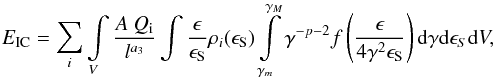16)where the overall emission is composed of the sum of two different contributions: SSC from jet photons (i = 1,ρ₁(ϵ_S) = ρ_jet) and EIC from star photons (i = 2,ρ₂(ϵ_S) = ρ_star).

In the above expression ϵ_S = hν_S is the seed photon energy, V is the volume over which to integrate the IC emission, i.e. the jet and other quantities are defined as follows: $\mathit{f}\left(\frac{\mathit{ϵ}}{\mathrm{4}{\mathit{\gamma }}^{\mathrm{2}}{\mathit{ϵ}}_{\mathrm{S}}}\right)\mathrm{=}\frac{\mathrm{2}}{\mathrm{3}}\left(\mathrm{1}\mathrm{-}\frac{\mathit{ϵ}}{\mathrm{4}{\mathit{\gamma }}^{\mathrm{2}}{\mathit{ϵ}}_{\mathrm{S}}}\right)\mathrm{for}\mathrm{0}\mathrm{\le }\frac{\mathit{ϵ}}{\mathrm{4}{\mathit{\gamma }}^{\mathrm{2}}{\mathit{ϵ}}_{\mathrm{S}}}\mathrm{\le }\mathrm{1}\mathit{,}$(17)and zero otherwise,

$\begin{array}{ccc}& & {\mathit{Q}}_{\mathit{i}}\mathrm{=}{\mathit{K}}_{\mathrm{I}}\mathrm{\times }\mathit{D}{\mathit{B}}_{\mathit{i}}\mathrm{\left(}{\mathit{\beta }}_{\mathrm{I}}\mathrm{\right)}\mathrm{+}{\mathit{K}}_{\mathrm{II}}\mathrm{\times }\mathit{D}{\mathit{B}}_{\mathit{i}}\mathrm{\left(}{\mathit{\beta }}_{\mathrm{II}}\mathrm{\right)}\\ & & \mathit{A}\mathrm{=}\frac{\mathrm{3}}{\mathrm{4}}\mathit{c}{\mathit{\sigma }}_{\mathrm{T}}\mathit{,}\end{array}$with the Thompson cross-section σ_T. The above expressions for plasma emission holds in the frame in which the plasma bulk motion is zero; the Doppler boosting (DB) term, DB_i, takes into account that the jet emitting plasma is moving with a speed v along the jet axis. Its general expression is written as $\begin{array}{ccc}\mathit{D}{\mathit{B}}_{\mathrm{i}}& \mathrm{=}& {\left[\frac{\mathrm{1}}{\mathrm{\Gamma }\mathrm{(}\mathrm{1}\mathrm{\pm }\mathit{\beta }\cos \mathit{\eta }\mathrm{)}}\right]}^{{\mathrm{ex}}_{\mathit{i}}}\mathit{,}\\ \mathrm{\Gamma }& \mathrm{=}& \frac{\mathrm{1}}{\sqrt{\mathrm{1}\mathrm{-}{\mathit{\beta }}^{\mathrm{2}}}}\mathit{,}\end{array}$(20)with β = v/c, and the possibility for a different injection velocity for each distribution is allowed, i.e. β = β_I for periastron distribution and β = β_II for apastron distribution. The parameter η is the angle between the observer’s line of sight and the jet axis (see Massi & Torricelli-Ciamponi 2014, for details). The DB exponent ex_i for IC radiation produced by stellar seed photons is different from that for synchrotron jet photons and, in particular, we have ex₁ = 3−α (see Ghisellini et al. 1985, where the spectral index α is defined with an opposite sign with respect to our definition) and ex₂ = 2 + p (Kaufman Bernadó et al. 2002).

The above expression (16) holds in the Thomson limit approximation, i.e. for γν_Sh<mc². This limit is not overpassed for the range of energies of Fermi-LAT data analysed in this paper and with the above described seed photon energy densities, if we set the free parameter γ₂ ≤ 7 × 10⁴.

The integral over the seed spectrum, i.e. on ϵ_S, is extended to all seed photons that can contribute to GeV emission. Since the function $\mathit{f}\left(\frac{\mathit{ϵ}}{\mathrm{4}{\mathit{\gamma }}^{\mathrm{2}}{\mathit{ϵ}}_{\mathrm{S}}}\right)$ is different from zero only in the interval [0,1], this condition shows that, given an electron distribution in a specific γ range, and a seed photon of energy ϵ_S, IC emission is different from zero only for energies, ϵ, such that 0 ≤ ϵ ≤ 4γ²ϵ_S.

The integration interval in dγ depends on the distance l along the jet axis since electrons lose energy while proceeding along the jet. Therefore, the integration range is γ_M(l = 1) = γ₂ and γ_m(l = 1) = γ₁ at the beginning of the jet, while for a generic distance we have

${\mathit{\gamma }}_{\mathrm{M}}\mathrm{\left(}\mathit{l}\mathrm{\right)}\mathrm{=}\mathit{\gamma }\mathrm{\left(}\mathit{l,}{\mathit{\gamma }}_{\mathrm{2}}\mathrm{\right)}{\mathit{\gamma }}_{\mathrm{m}}\mathrm{\left(}\mathit{l}\mathrm{\right)}\mathrm{=}\mathit{\gamma }\mathrm{\left(}\mathit{l,}{\mathit{\gamma }}_{\mathrm{1}}\mathrm{\right)}\mathit{,}$where these functions are specified by Eq. (26) in the next section.

3.5. Accelerated electron survival

As outlined in various parts of this section, relativistic electrons lose energy with time, i.e. on their way along the jet, owing to different types of losses and hence their γ values decrease. The standard way to take electron energy losses into account requires the solution of the following equation (see e.g. Longair 1994): $\frac{\mathit{\partial \gamma }}{\mathit{\partial t}}\mathrm{=}\mathrm{-}\mathit{\gamma }\frac{\mathrm{2}{\mathit{a}}_{\mathrm{1}}}{\mathrm{3}\mathit{t}}\mathrm{-}\mathit{W}{\mathit{\gamma }}^{\mathrm{2}}{\mathit{U}}_{\mathit{B}}\mathrm{-}\mathit{W}{\mathit{\gamma }}^{\mathrm{2}}{\mathit{U}}_{\mathrm{jet}}\mathrm{-}\mathit{W}{\mathit{\gamma }}^{\mathrm{2}}{\mathit{U}}_{\mathrm{star}}\mathit{.}$(21)The first term on the right-hand side takes adiabatic losses into account, as derived by Kaiser (2006) for the specific jet configuration we are using in this paper. The following terms account for synchrotron and IC losses due to electron interactions with synchrotron jet photons (SSC) and star photons (EIC). In the above expression $\mathit{W}\mathrm{=}\mathrm{4}{\mathit{\sigma }}_{\mathrm{T}}\mathit{/}\mathrm{\left(}\mathrm{3}{\mathit{m}}_{\mathrm{e}}\mathit{c}\mathrm{\right)}\mathrm{=}\mathrm{3.2}\mathrm{\times }{\mathrm{10}}^{-8}\frac{\mathrm{s}\mathrm{cm}}{\mathrm{g}}$, the term ${\mathit{U}}_{\mathit{B}}\mathrm{\left(}\mathit{l}\mathrm{\right)}\mathrm{=}\frac{{\mathit{B}}_{\mathrm{0}}^{\mathrm{2}}}{\mathrm{8}\mathit{\pi }}{\mathit{l}}^{\mathrm{-}{\mathit{a}}_{\mathrm{2}}}\mathrm{[}\mathrm{erg}\hspace{0.17em}\mathrm{c}{\mathrm{m}}^{-3}\mathrm{]}$(22)defines the magnetic energy density, while the two terms

$\begin{array}{ccc}& & {\mathit{U}}_{\mathrm{jet}}\mathrm{\left(}\mathit{l,}\mathrm{\Phi }\mathrm{\right)}\mathrm{=}\frac{\mathrm{4}\mathit{\pi }}{\mathit{c}}\mathrm{\int }{\mathit{I}}_{\mathit{\nu }}\mathrm{d}\mathit{\nu }\mathrm{[}\mathrm{erg}\hspace{0.17em}\mathrm{c}{\mathrm{m}}^{-3}\mathrm{]}\\ & & {\mathit{U}}_{\mathrm{star}}\mathrm{\left(}\mathit{l,}\mathrm{\Phi }\mathit{,}\mathrm{\Theta }\mathrm{\right)}\mathrm{=}\mathrm{\int }\frac{{\mathit{B}}_{\mathit{\nu }}\mathrm{\left(}{\mathit{T}}_{\mathrm{\ast }}\mathrm{\right)}}{\mathit{c}}\frac{\mathit{\pi }{\mathit{R}}_{\mathrm{\ast }}^{\mathrm{2}}}{{\mathit{d}}_{\mathrm{[}\mathrm{jet}\mathrm{-}\mathrm{star}\mathrm{]}}^{\mathrm{2}}}\mathrm{d}\mathit{\nu }\mathrm{[}\mathrm{erg}\hspace{0.17em}\mathrm{c}{\mathrm{m}}^{-3}\mathrm{]}\end{array}$describe synchrotron photon density and star photon density inside the jet.

The most likely magnetic configuration in a jet is a helical magnetic field configuration with both the parallel and perpendicular components. Following Kaiser’s model we can reproduce B ~ B_∥ by setting a₂ = 2 and B ~ B_⊥ with a₂ = 1. In our framework, as in Massi & Torricelli-Ciamponi (2014), we set for our model a₁ = 1, corresponding to a jet with a constant opening angle, and a₂ = 2, corresponding to a parallel magnetic field, since we found comparable solutions for the two configurations of B as in Massi & Torricelli-Ciamponi (2014).

Equation (21) is a first order differential equation of the Bernoulli type, which can be easily integrated between t and t_min to give $\mathit{\gamma }\mathrm{\left(}\mathit{t}\mathrm{\right)}\mathrm{=}\frac{\mathit{g}{\mathit{t}}^{\mathrm{-}\mathrm{2}\mathit{/}\mathrm{3}}}{{\mathit{t}}_{\min }^{\mathrm{-}\mathrm{2}\mathit{/}\mathrm{3}}\mathrm{+}\mathit{Wg}{\mathrm{\int }}_{{\mathit{t}}_{\min }}^{\mathit{t}}{\mathit{t}}^{\mathrm{-}\mathrm{2}\mathit{/}\mathrm{3}}\mathrm{[}{\mathit{U}}_{\mathit{B}}\mathrm{+}{\mathit{U}}_{\mathrm{jet}}\mathrm{+}{\mathit{U}}_{\mathrm{star}}\mathrm{]}\mathrm{d}\mathit{t}}\mathit{,}$(25)where g = γ(t_min). Setting t_min = x₀/ (Γβc) for electrons starting at l = 1, i.e. at the jet basis, x₀, and t = x₀l/ (Γβc) as the time at which electrons attain the generic position lx₀ along the jet axis, Eq. (25) can be rewritten in terms of the spatial coordinate along the jet axis as $\mathit{\gamma }\mathrm{\left(}\mathit{l,g}\mathrm{\right)}\mathrm{=}\frac{\mathit{g}{\mathit{l}}^{\mathrm{-}\mathrm{2}\mathit{/}\mathrm{3}}}{\mathrm{1}\mathrm{+}\mathit{W}\frac{{\mathit{x}}_{\mathrm{0}}}{\mathrm{\Gamma }\mathit{\beta c}}\mathit{g}\left\{{\mathrm{\int }}_{\mathrm{1}}^{\mathit{l}}{\mathit{l}}^{\mathrm{-}\mathrm{2}\mathit{/}\mathrm{3}}\mathrm{[}{\mathit{U}}_{\mathit{B}}\mathrm{+}{\mathit{U}}_{\mathrm{jet}}\mathrm{+}{\mathit{U}}_{\mathrm{star}}\mathrm{]}\mathrm{d}\mathit{l}\right\}}\mathrm{·}$(26)This expression shows how γ evolves along the jet when subject to adiabatic, synchrotron, and IC losses.

Following Eq. (26) each initial Lorentz factor value, g, decreases along the jet so that the entire initial distribution shifts to lower energies. In particular, choosing γ(t_min) = g = γ₂, we can determine how the upper limit of the distribution evolves along the jet, i.e. γ_M(l) = γ(l,γ₂). This evolution is shown in Fig. 3b. In our present model we account for all types of energy losses described in this section through the use of a different upper limit cut-off of the electron distribution for each position l along the jet axis; this is the same method used by Kaiser (2006) only for adiabatic and synchrotron losses. As stated in Sect. 3.1, losses due to adiabatic jet expansion have been taken into account also in the electron density distribution (see Eq.(3)).

Using the above cited Eq. (13), we can derive the jet length as the position along the jet axis above which electron energies are too low to emit the observed radio flux. In fact, for B = B₀l^-2 and with a magnetic field value at the jet basis of B₀ = 5.1 G (as results from our present model), it is possible to have synchrotron radiation at ν = 15 GHz (OVRO observations) only if the electron distribution extends up to ${\mathit{\gamma }}_{\mathit{M}}\mathrm{\left(}\mathit{l}\mathrm{\right)}\mathit{>}{\left[\frac{\mathit{\nu }{\mathit{l}}^{\mathrm{2}}}{\mathrm{1.8}\mathrm{\times }{\mathrm{10}}^{\mathrm{6}}{\mathit{B}}_{\mathrm{0}}}\right]}^{\mathrm{1}\mathit{/}\mathrm{2}}\mathrm{\approx }\mathrm{40}\mathit{l}\mathit{.}$(27)Condition (27) is drawn as a black line in Fig. 3 b; its intersection with the red (blue) line describing the γ decrease induced by losses at periastron (apastron) defines the jet length L ~ 1.2 (L ~ 25). At apastron it is evident that the jet length (L ~ 25), and hence the radio emission, is not limited by radiative losses.

4. Observations and data reduction

We compare the model output data to observational data at radio and GeV wavelengths. The databases that we use are the OVRO monitoring at 15 GHz ranging from MJD 54 684 to MJD 56 794 (2008 Aug. 6 to 2014 May 17), and GeV γ-ray data from the Fermi-LAT in the energy range 0.1−3.0 GeV from MJD 54 682 to MJD 57 450 (2008 Aug. 4 to 2016 March 3).

The calibration of radio OVRO data is described in Massi et al. (2015).

We used version v10r0p5 of the Fermi ScienceTools¹ for the analysis of Fermi-LAT data. We used the instrument response function P8R2_SOURCE_V6 and the corresponding model gll_iem_v06.fits for the Galactic diffuse emission and the template iso_P8R2_SOURCE_V6_v06.txt. Model files were created automatically with the script make3FGLxml.py² from the third Fermi-LAT point source catalogue (The Fermi-LAT Collaboration 2015). The spectral shape of LS I + 61°303 in the GeV regime is a power law with an exponential cut-off at 4−6 GeV (Abdo et al. 2009; Hadasch et al. 2012). Here we restrict our analysis to the power law part of the GeV emission by fitting the source with $\frac{\mathrm{d}\mathit{n}}{\mathrm{d}\mathit{E}}\mathrm{=}{\mathit{n}}_{\mathrm{0}}{\left(\frac{\mathit{E}}{{\mathit{E}}_{\mathrm{0}}}\right)}^{\mathrm{-}\mathit{\alpha }\mathrm{+}\mathit{\beta }\log \left(\mathit{E}\mathit{/}{\mathit{E}}_{\mathrm{b}}\right)}\left[\frac{\mathrm{counts}}{\mathrm{c}{\mathrm{m}}^{\mathrm{2}}\hspace{0.17em}\hspace{0.17em}\mathrm{s}\mathrm{d}\mathit{E}}\right]\mathit{,}$(28)where all parameters are left free for the fit and including data in the energy range E = 0.1−3 GeV. All other sources within a radius of 10° and the Galactic diffuse emission were left free for the fit. All sources between 10−15° were fixed to their catalogue values. The light curves were computed by performing this fit for every time bin of width one day for Fermi-LAT data from 2008 August 8 (MJD 54 684) till 2016 March 3 (MJD 57 450). On average, the test statistic for LS I + 61°303 was 40, which corresponds to a detection of the source at the 6.3σ level on average in each time bin.

The search for periodicities in the light curves is carried out with the UK Starlink package, implementing the Lomb-Scargle algorithm (Lomb 1976; Scargle 1982). The procedure is the same as outlined in Massi & Jaron (2013).

4.1. Consistency with previous results

Jaron & Massi (2014) found that the GeV data from LS I + 61°303 observed by the Fermi-LAT are modulated by P₁ and P₂ in the orbital phase interval Φ = 0.5−1.0 (apastron), but by only P₁ in Φ = 0.0−0.5 (periastron) (see their Fig. 3). Their analysis was performed with Pass 7 Fermi-LAT data, using the energy range 0.1−300 GeV, and for the time interval MJD 54 683−56 838. We use Pass 8 Fermi-LAT data and restrict the energy range to 0.1−3.0 GeV. It is therefore important to verify how the data processed with the new method compare to the previous data. We apply the timing analysis to the data processed with the new method as in Jaron & Massi (2014). The result is shown in the top panel of Fig. 4. Since we use a time bin of one day for the likelihood analysis, Figs. 3e and h in Jaron & Massi (2014) are the figures to use for comparison. Clearly the result of Jaron & Massi (2014) is confirmed here; in our Fig. 4a the only significant feature is the peak at the orbital period P₁, whereas in Fig. 4 b there is not only a peak at P₁ but also a highly significant peak at P₂. This result shows that the timing characteristic reported by Jaron & Massi (2014) is a feature from the emission in the range 0.1−3 GeV.

4.2. Influence of the Θ interval on P₂

Applying the same timing analysis to all available Fermi-LAT data ranging from MJD 54682 to MJD 57450 (Θ = 6.8−8.8) we obtain the result presented in the bottom panel of Fig. 4. In Fig. 4c, which shows the Lomb-Scargle periodogram for the periastron data, the orbital period P₁ has increased its power and stands out a bit more significantly over the noise when compared to Fig. 4a. However, the P₂ feature in Fig. 4d has decreased its power and its relative importance with respect to P₁ drops to about 1/2, when it was 3/4 for the narrower time range shown in Fig. 4b.

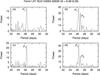Fig. 4 Timing analysis of Pass 8 Fermi-LAT data, energy range 0.1−3.0 GeV. a), b) Time interval MJD 54 683−56 838 (same epoch as used in Jaron & Massi 2014, where they used Pass 7 data and the energy range 0.1−300 GeV). The result of the timing analysis is confirmed (compare Fig. 3 in Jaron & Massi 2014): a) periastron, only P1; and b) apastron, P1 and P2. c), d) Time interval is 54 683−57 450: c) periastron, only P1; and d) apastron, P1 and P2, but with less power than in b).

Which data are causing this decline in the power of P₂? In order to find out we remove a certain interval of the long-term modulation from the data in the sense that we delete data for which Θ = 0.0−0.1, 0.1−0.2,...,0.9−1.0 and perform Lomb-Scarge timing analysis on the remaining data. In Fig. 5 the resulting powers of P₁ and P₂ are plotted for the different Θ intervals removed from the data. While the power of P₁ is only slightly affected by the choice of the removed Θ interval in a random manner, the power of P₂ is clearly dependent on the removed Θ interval in a stronger and systematic way. We find that P₂ gains the most power if we remove the data from the interval Θ = 0.5−0.6, which is indicated by the grey areas in Fig. 6, where we plot all Fermi-LAT data from the orbital phase interval Φ = 0.5−1.0 (i.e. apastron) and averaged over one orbit. The resulting periodogram, plotted in Fig. 1c, shows two peaks at P₁ and P₂ with equal power.

Something in the interval around Θ ~ 0.5 affects the precessing jet and consequently the timing analysis. In the interval 2006−2007, which corresponds to Θ_integer = 6.38−6.60, there was strong (15%−20% Crab nebula) TeV flaring activity (see Aliu et al. 2013 and references therein) as in 2014 (corresponding to Θ_integer = 8.36 (>25% Crab nebula) Archambault et al. 2016). TeV flaring activity was found to be consistent with the long-term period (Ahnen et al. 2016). The GeV flares we found perturbing the precessing jet and likely related to the TeV flares should then follow the same periodicity. This finding suggests a link to be explored between the high energy phenomena and the radio transient in LS I + 61°303. This bursting phase of optically thin emission present in LS I + 61°303 as in other microquasars (Massi & Torricelli-Ciamponi 2014; Zimmermann et al. 2015) is in fact associated with shocks travelling in the jet some days after the optically thick outburst of the steady jet (Massi 2014, Fig. 3).

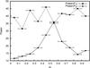Fig. 5 Test on the Θ interval that corrupts the timing analysis. In this plot the powers of P1 and P2 resulting from Lomb-Scargle timing analysis are plotted as a function of the Θ interval removed from the data, where interval is indicated with horizontal error bars. While the power of P1 is only affected very little and in a random way, the power of P2 shows a systematic trend peaking at Θ = 0.5−0.6.

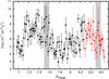Fig. 6 All Fermi-LAT data from the orbital phase interval Φ = 0.5−1.0, i.e. apastron vs. [(t−t0)/1626]. Data up to MJD 56 838 (the time interval in Jaron & Massi 2014) are plotted in black; data newer than that appear in red. The long-term amplitude modulation is clearly visible. The two grey areas indicate the Θ intervals that are removed from the data for the analysis of this paper.

5. Results

In this section we compare the observations with model data calculated by our physical model of a precessing (P₂) jet periodically (P₁) refilled in two different parts of the orbit, with relativistic electrons and emitting synchrotron emission in the radio band (Eq. (1) in Massi & Torricelli-Ciamponi 2014) and inverse Compton emission in the GeV band (Eq. (15)). Model data were fitted to the observations versus time with the additional constraint that the periodograms of model data have to reproduce the periodograms of the observations. The fit results for the two ejections are given in Table 1. The results of the fit for the jet are given in Table 2.

Figure 3 shows the resulting shape of the two electron distributions injected around periastron and towards apastron. The relativistic electron density K_I is larger than K_II as for the accretion peaks of Fig. 6 in Marti & Paredes (1995). The resulting mean energy injected per second in the form of relativistic electrons is L_rel = 8 × 10³⁵ erg/s. This value is consistent with the observed gamma-ray luminosity, 7 × 10³⁵ erg/s, resulting from the Fermi-LAT data.

The resulting jet lengths, L, are derived by the analysis of the energetic losses of the electrons; Fig. 3b reports how the maximum electron Lorentz factor evolves along the jet axis and where it attains a value that is too low to be able to produce radio emission.

We performed timing analysis of Fermi-LAT observations and our model data; Fig. 1 shows the results. The observed γ-ray flux is modulated by only the orbital period P₁ at periastron (Fig. 1a). Also the model data are only modulated by the same period P₁ (Fig. 1b). At apastron, both observational and model data are not only modulated by P₁ but also by P₂ (Figs. 1c and d). Radio observations and model radio data both show the two features at P₁ and P₂ (Figs. 1e and f).

Fig. 7 Results of the model in comparison with the observations. a) Comparison of the model GeV output (red) with the observations by the Fermi-LAT (black), the energy range is 0.1−3.0 GeV in both cases and the time interval is MJD 54 682−57450. The observed Fermi-LAT light curve, here folded on the orbital period P1 = 26.4960 days, shows two peaks. Assuming two electron injections along the orbit, the shape of the orbital modulation of this observed GeV light curve is reproduced. b) Comparison of the model radio output (red) with the observations by OVRO (black), both at 15 GHz spanning the time interval MJD 54 909−56 794. The observed light curve, folded on the orbital period P1, shows only one peak along the orbit. The model reproduces this characteristic apastron peak even though two electron injections are taken into account.

The folded light curves for radio (OVRO) and γ-ray data (Fermi-LAT) are shown in Fig. 7. Even if K_I is larger than K_II (Fig. 3), in the right panel of Fig. 7 one sees only the large radio outburst at apastron for both observations and the model data.

Concerning Fermi-LAT data, the two-peaked structure is present in both observations and model. The two-peaked structure is above an offset of 5 × 10^-7 cm^-2 s^-1. The origin of the offset could be SSC of optical photons produced not in the jet but in the hot flow that fills the inner part of the accretion flow. Indeed, optical observations by Casares et al. (2005) indicated an extra contribution to the stellar emission that the authors attributed possibly to the disk around the Be star. Today it is suggested that in X-ray binaries optical synchrotron radiation might come from the hot accretion flow (Poutanen & Veledina 2014). The SSC emission of this optical radiation, invoked to explain the MeV tail in the hard state of Cygnus X-1 (Poutanen & Veledina 2014), seems to extend to GeV here, as the LS I + 61°303 spectrum from 0.01−1000 MeV in Fig. 5 by Tavani et al. (1996) suggests. Optical observations by Mendelson & Mazeh (1989) measured two variations at periastron and towards apastron. Our left panel of Fig. 7, which shows two peaks above the large offset, fits and completes a scenario in which the offset could be associated with the SSC of optical photons of the hot accretion flow and the two peaks to SSC and EIC of jet and stellar photons scattered by electrons of the jet. Concerning this jet component, the main contribution comes from the SSC reprocessing for the parameter range resulting from the above fit. The relative importance of SSC emission with respect to EIC emission, even if always in favour of the former, changes not only with the orbital phase Φ, but also shows a long-term modulation with Θ.

6. Conclusions

The open issue this paper aimed to address is why the long-term modulation does not affect the gamma-ray emission of LS I + 61°303 at periastron, or equivalently why P₂ is missing in the periodogram of the gamma-ray emission at periastron. In addition, we wanted to understand whether there is any relationship between this lack of P₂ in the gamma-ray emission and the absence of a radio outburst at periastron.

We modelled the observed flux in terms of synchrotron and IC emission of a precessing jet (with period P₂) periodically (P₁) refilled, twice along the orbit, with relativistic electrons.

The model solution implies that the ejection at periastron, where the compact object is embedded in the densest part of the Be wind, is indeed the larger of the two ejections. The larger inertia, because of the higher accretion rate and the dense environment where the jet propagates, may explain why the jet at periastron is slow; the model solution gives at periastron β = 0.006 ± 0.004.

This slow dense jet, which at periastron is embedded in the stellar photon field, suffers from strong energetic losses via IC, i.e. electrons upscatter optical/UV photons to gamma-ray energy and by doing that quickly lose their energy. This explains why at periastron there is strong gamma-ray emission and only negligible radio emission. In fact, we find that the electrons in the jet at periastron reduce their Lorentz factor under the level at which they can emit radio (15 GHz) synchrotron radiation already at the very short distance of L = 1.20 ± 0.01. That corresponds to x = Lx₀ = 3.0 × 10⁶r_s (for M_BH = 3 M_⊙), that is barely after the acceleration/collimation region of a jet that is at ~10^5.5r_s (Marscher 2006). For the second minor ejection towards apastron the length of the jet results to be L = 25 ± 2, i.e. x = 6.3 × 10⁷r_s and β = 0.5 ± 0.2.

The observed flux is S₀(P₁,P₂) = S_i(P₁)DB(P₂). The intrinsic flux S_i = f(P₁) is due to IC and synchrotron processes. The DB is a function of βcos(η(f(P₂))). In fact, the precession of the jet periodically changing the angle η between the jet axis and line of sight changes the DB. The low velocity at periastron gives rise to a small Doppler factor and hence to a negligible dependency on P₂. As a result, the γ-ray flux at periastron is neither modulated by the long-term periodicity (Ackermann et al. 2013) owing to the beating between P₁ and P₂ (Jaron & Massi 2014) nor does P₂ appear in the timing analysis. In fact, each period, P₁ and P₂, only appears in the timing analysis when the related term (S_i(P₁) or DB(P₂)) is significant. At apastron, the larger velocity creates larger DB variations, P₂ appears in the timing analysis, and radio and gamma-ray emission show the long-term periodicity.

Acknowledgments

We thank Eduardo Ros and Karl Menten for reading the manuscript. We thank Bindu Rani and Robin Corbet for useful discussions about likelihood analysis of Fermi-LAT data. We thank Alan Marscher for useful discussions about jet acceleration. Helge Rottmann provided us with computing power. This work has made use of public Fermi data obtained from the High Energy Astrophysics Science Archive Research Center (HEASARC), provided by NASA Goddard Space Flight Center. The OVRO 40 m Telescope Monitoring Program is supported by NASA under awards NNX08AW31G and NNX11A043G, and by the NSF under awards AST-0808050 and AST-1109911.

References

All Tables

All Figures

Fig. 1 Top: sketch of the stellar system LS I + 61°303. We assume two ejections of relativistic electrons along the orbit as in Bosch-Ramon et al. (2006). The two ejections refill the conical precessing jet defined in Massi & Torricelli-Ciamponi (2014). The electrons emit by synchrotron and IC processes. The resulting jet parameters are given in Table 2. The ejection at periastron gives rise to gamma-ray emission only and the periodogram of this emission only shows P1, the orbital period. The ejection towards apastron is associated with gamma-ray and radio emission. The periodograms for both emissions show two features, at P1 and P2, the precession period of the jet. a) Lomb-Scargle periodogram for Fermi-LAT data from the orbital phase interval Φ = 0.0−0.5 (periastron). The orbital period P1 is clearly detected. b) Lomb-Scargle periodogram of the model gamma-ray data (IC) from the orbital phase interval Φ = 0.0−0.5 (periastron). The orbital period P1 is the only peak, in agreement with the observations. c) In the orbital phase interval Φ = 0.5−1.0 (apastron), there is a peak at the precession period P2 in addition to the orbital period P1. d) The two peaks at P1 and P2 in the apastron data are reproduced by the model. e) Lomb-Scargle periodogram for OVRO radio data for the whole orbital phase interval. Both P1 and P2 are present. f) Lomb-Scargle periodogram of the model radio data (synchrotron emission). Both peaks are reproduced by the model.

In the text

Fig. 2 Top: radio light curve at 2 (red circles) and 8 GHz (blue squares) observed by the GBI from MJD 50 154.6 until 50 175.7 (orbital phase Φ = 0.1−1.0), averaged over one day. Bottom: radio spectral index α of the radio fluxes shown in the top panel clearly follows a two-peaked trend. One peak is during the large apastron radio outburst, which features a flat or inverted (α ≥ 0) spectrum during its rise. The other peak of the spectral index occurs at Φ = 0.25, i.e. at periastron, revealing that the spectrum becomes flattish (α ≈ 0) during this orbital phase as well (Massi & Kaufman Bernadó 2009).

In the text

Fig. 3 a) Orbital modulation of the electron density assumed in the model, as defined in Sect. 3.1. The two ejections are given at Φ = 0.35 and at Φ = 0.58. b) The maximum value of the Lorentz factor γ of the electrons as a function of the position l along the jet for the two ejections. The black curve is a plot of the minimum γ (Eq. (27)) necessary for the production of radio emission at 15 GHz for an initial magnetic field B0 = 5 G. The intersection point of the black curve with the red and blue lines defines the length of the jet at periastron and that of the jet towards apastron, respectively.

In the text

Fig. 4 Timing analysis of Pass 8 Fermi-LAT data, energy range 0.1−3.0 GeV. a), b) Time interval MJD 54 683−56 838 (same epoch as used in Jaron & Massi 2014, where they used Pass 7 data and the energy range 0.1−300 GeV). The result of the timing analysis is confirmed (compare Fig. 3 in Jaron & Massi 2014): a) periastron, only P1; and b) apastron, P1 and P2. c), d) Time interval is 54 683−57 450: c) periastron, only P1; and d) apastron, P1 and P2, but with less power than in b).

In the text

Fig. 5 Test on the Θ interval that corrupts the timing analysis. In this plot the powers of P1 and P2 resulting from Lomb-Scargle timing analysis are plotted as a function of the Θ interval removed from the data, where interval is indicated with horizontal error bars. While the power of P1 is only affected very little and in a random way, the power of P2 shows a systematic trend peaking at Θ = 0.5−0.6.

In the text

	Fig. 6 All Fermi-LAT data from the orbital phase interval Φ = 0.5−1.0, i.e. apastron vs. [(t−t0)/1626]. Data up to MJD 56 838 (the time interval in Jaron & Massi 2014) are plotted in black; data newer than that appear in red. The long-term amplitude modulation is clearly visible. The two grey areas indicate the Θ intervals that are removed from the data for the analysis of this paper.
In the text

Fig. 7 Results of the model in comparison with the observations. a) Comparison of the model GeV output (red) with the observations by the Fermi-LAT (black), the energy range is 0.1−3.0 GeV in both cases and the time interval is MJD 54 682−57450. The observed Fermi-LAT light curve, here folded on the orbital period P1 = 26.4960 days, shows two peaks. Assuming two electron injections along the orbit, the shape of the orbital modulation of this observed GeV light curve is reproduced. b) Comparison of the model radio output (red) with the observations by OVRO (black), both at 15 GHz spanning the time interval MJD 54 909−56 794. The observed light curve, folded on the orbital period P1, shows only one peak along the orbit. The model reproduces this characteristic apastron peak even though two electron injections are taken into account.

In the text

References

- Abdo, A. A., Ackermann, M., Ajello, M., et al. 2009, ApJ, 701, L123 [NASA ADS] [CrossRef] [Google Scholar]
- Ackermann, M., Ajello, M., Ballet, J., et al. 2013, ApJ, 773, L35 [NASA ADS] [CrossRef] [Google Scholar]
- Ahnen, M. L., Ansoldi, S., Antonelli, L. A., et al. 2016, A&A, 591, A76 [NASA ADS] [CrossRef] [EDP Sciences] [Google Scholar]
- Aliu, E., Archambault, S., Behera, B., et al. 2013, ApJ, 779, 88 [NASA ADS] [CrossRef] [Google Scholar]
- Archambault, S., Archer, A., Aune, T., et al. 2016, ApJ, 817, L7 [NASA ADS] [CrossRef] [Google Scholar]
- Bondi, H., & Hoyle, F. 1944, MNRAS, 104, 273 [NASA ADS] [CrossRef] [Google Scholar]
- Bosch-Ramon, V., Paredes, J. M., Romero, G. E., & Ribó, M. 2006, A&A, 459, L25 [NASA ADS] [CrossRef] [EDP Sciences] [Google Scholar]
- Casares, J., Ribas, I., Paredes, J. M., Martí, J., & Allen de Prieto, C. 2005, MNRAS, 360, 1105 [NASA ADS] [CrossRef] [Google Scholar]
- Chernyakova, M., Neronov, A., & Walter, R. 2006, MNRAS, 372, 1585 [NASA ADS] [CrossRef] [Google Scholar]
- Dhawan, V., Mioduszewski, A., & Rupen, M. 2006, VI Microquasar Workshop: Microquasars and Beyond, 52.1 [Google Scholar]
- D’Aì, A., Cusumano, G., La Parola, V., Segreto, A., & Mineo, T. 2016, MNRAS, 456, 1955 [NASA ADS] [CrossRef] [Google Scholar]
- Dubus, G. 2006, A&A, 456, 801 [NASA ADS] [CrossRef] [EDP Sciences] [Google Scholar]
- Fender, R. P., Garrington, S. T., McKay, D. J., et al. 1999, MNRAS, 304, 865 [NASA ADS] [CrossRef] [Google Scholar]
- Ghisellini, G., Maraschi, L., & Treves, A. 1985, A&A, 146, 204 [NASA ADS] [Google Scholar]
- Ginzburg, V. L., & Syrovatski, S. I. 1965, ARA&A, 3, 297 [NASA ADS] [CrossRef] [Google Scholar]
- Gregory, P. C. 2002, ApJ, 575, 427 [NASA ADS] [CrossRef] [Google Scholar]
- Gregory, P. C., & Neish, C. 2002, ApJ, 580, 1133 [NASA ADS] [CrossRef] [Google Scholar]
- Gregory, P. C., Taylor, A. R., Crampton, D., et al. 1979, AJ, 84, 1030 [NASA ADS] [CrossRef] [Google Scholar]
- Gregory, P. C., Peracaula, M., & Taylor, A. R. 1999, ApJ, 520, 376 [NASA ADS] [CrossRef] [Google Scholar]
- Hadasch, D., Torres, D. F., Tanaka, T., et al. 2012, ApJ, 749, 54 [NASA ADS] [CrossRef] [Google Scholar]
- Harmanec, P. 1984, Bull. Astron. Inst. Czechoslovakia, 35, 164 [Google Scholar]
- Harrison, F. A., Ray, P. S., Leahy, D. A., Waltman, E. B., & Pooley, G. G. 2000, ApJ, 528, 454 [NASA ADS] [CrossRef] [Google Scholar]
- Jaron, F., & Massi, M. 2013, A&A, 559, A129 [NASA ADS] [CrossRef] [EDP Sciences] [Google Scholar]
- Jaron, F., & Massi, M. 2014, A&A, 572, A105 [NASA ADS] [CrossRef] [EDP Sciences] [Google Scholar]
- Kaiser, C. R. 2006, MNRAS, 367, 1083 [NASA ADS] [CrossRef] [Google Scholar]
- Kaufman Bernadó, M. M., Romero, G. E., & Mirabel, I. F. 2002, A&A, 385, L10 [NASA ADS] [CrossRef] [EDP Sciences] [Google Scholar]
- Longair, M. S. 1994, High Energy Astrophysics (Cambridge Univ. Press) [Google Scholar]
- Lomb, N. R. 1976, Ap&SS, 39, 447 [NASA ADS] [CrossRef] [Google Scholar]
- Marscher, A. P. 2006, Chin. J. Astron. Astrophys. Suppl., 6, 262 [NASA ADS] [CrossRef] [Google Scholar]
- Marti, J., & Paredes, J. M. 1995, A&A, 298, 151 [NASA ADS] [Google Scholar]
- Massi, M. 2014, Proc. 12th European VLBI Network Symp. and Users Meeting (EVN 2014). 7−10 October 2014. Cagliari, Italy. Online at <A href=”http://pos.sissa.it/cgi-bin/reader/conf.cgi?confid=230”>http://pos.sissa.it/cgi-bin/reader/conf.cgi?confid=230</A>, 62 [Google Scholar]
- Massi, M., & Jaron, F. 2013, A&A, 554, A105 [NASA ADS] [CrossRef] [EDP Sciences] [Google Scholar]
- Massi, M., & Kaufman Bernadó, M. 2009, ApJ, 702, 1179 [NASA ADS] [CrossRef] [Google Scholar]
- Massi, M., & Torricelli-Ciamponi, G. 2014, A&A, 564, A23 [NASA ADS] [CrossRef] [EDP Sciences] [Google Scholar]
- Massi, M., & Torricelli-Ciamponi, G. 2016, A&A, 585, A123 [NASA ADS] [CrossRef] [EDP Sciences] [Google Scholar]
- Massi, M., Paredes, J. M., Estalella, R., & Felli, M. 1993, A&A, 269, 249 [NASA ADS] [CrossRef] [Google Scholar]
- Massi, M., Ribó, M., Paredes, J. M., et al. 2002, Proc. 6th EVN Symp., 279 [Google Scholar]
- Massi, M., Ribó, M., Paredes, J. M., et al. 2004, A&A, 414, L1 [NASA ADS] [CrossRef] [EDP Sciences] [Google Scholar]
- Massi, M., Ros, E., & Zimmermann, L. 2012, A&A, 540, A14 [Google Scholar]
- Massi, M., Ros, E., Zimmermann, L., & Torricelli-Ciamponi, G. 2013, 370 Years of Astronomy in Utrecht, 470, 373 [Google Scholar]
- Massi, M., Jaron, F., & Hovatta, T. 2015, A&A, 575, L9 [NASA ADS] [CrossRef] [EDP Sciences] [Google Scholar]
- Maraschi, L., Treves, A., & Tanzi, E. G. 1981, ApJ, 248, 1010 [NASA ADS] [CrossRef] [Google Scholar]
- Mendelson, H., & Mazeh, T. 1989, MNRAS, 239, 733 [NASA ADS] [Google Scholar]
- Paredes, J. M., Estalella, R., & Rius, A. 1990, A&A, 232, 377 [NASA ADS] [Google Scholar]
- Paredes, J. M., Marziani, P., Marti, J., et al. 1994, A&A, 288, 519 [NASA ADS] [Google Scholar]
- Paredes-Fortuny, X., Ribó, M., Bosch-Ramon, V., et al. 2015, A&A, 575, L6 [NASA ADS] [CrossRef] [EDP Sciences] [Google Scholar]
- Poutanen, J., & Veledina, A. 2014, Space Sci. Rev., 183, 61 [NASA ADS] [CrossRef] [Google Scholar]
- Ray, P. S., Foster, R. S., Waltman, E. B., Tavani, M., & Ghigo, F. D. 1997, ApJ, 491, 381 [NASA ADS] [CrossRef] [Google Scholar]
- Romero, G. E., Okazaki, A. T., Orellana, M., & Owocki, S. P. 2007, A&A, 474, 15 [NASA ADS] [CrossRef] [EDP Sciences] [Google Scholar]
- Rybicki, G. B., & Lightman, A. P. 1986, Radiative Processes in Astrophysics (Wiley-VCH), 400 [Google Scholar]
- Scargle, J. D. 1982, ApJ, 263, 835 [NASA ADS] [CrossRef] [Google Scholar]
- Štefl, S., Rivinius, T., Carciofi, A. C., et al. 2009, A&A, 504, 929 [NASA ADS] [CrossRef] [EDP Sciences] [Google Scholar]
- Tavani, M., Fruchter, A., Zhang, S. N., et al. 1996, ApJ, 473, L103 [NASA ADS] [CrossRef] [Google Scholar]
- Taylor, A. R., & Gregory, P. C. 1982, ApJ, 255, 210 [NASA ADS] [CrossRef] [Google Scholar]
- Taylor, A. R., Kenny, H. T., Spencer, R. E., & Tzioumis, A. 1992, ApJ, 395, 268 [NASA ADS] [CrossRef] [Google Scholar]
- Taylor, A. R., Dougherty, S. M., Scott, W. K., Peracaula, M., & Paredes, J. M. 2000, Astrophysical Phenomena Revealed by Space VLBI, 223 [Google Scholar]
- The Fermi-LAT Collaboration 2015, ApJS, 218, 23 [Google Scholar]
- Zamanov, R. K., Martí, J., Paredes, J. M., et al. 1999, A&A, 351, 543 [NASA ADS] [Google Scholar]
- Zamanov, R., Stoyanov, K., Martí, J., et al. 2013, A&A, 559, A87 [NASA ADS] [CrossRef] [EDP Sciences] [Google Scholar]
- Zimmermann, L., Fuhrmann, L., & Massi, M. 2015, A&A, 580, L2 [NASA ADS] [CrossRef] [EDP Sciences] [Google Scholar]