| Issue |
A&A
Volume 584, December 2015
|
|
|---|---|---|
| Article Number | A2 | |
| Number of page(s) | 27 | |
| Section | Galactic structure, stellar clusters and populations | |
| DOI | https://doi.org/10.1051/0004-6361/201526336 | |
| Published online | 13 November 2015 | |
KMOS view of the Galactic centre
I. Young stars are centrally concentrated⋆,⋆⋆,⋆⋆⋆
1 European Southern Observatory (ESO), Karl-Schwarzschild-Straße 2, 85748 Garching, Germany
e-mail: This email address is being protected from spambots. You need JavaScript enabled to view it.
2 Max-Planck-Institut für Astronomie, Königsstuhl 17, 69117 Heidelberg, Germany
3 Instituto de Astrofísica de Andalucía (CSIC), Glorieta de la Astronomía s/n, 18008 Granada, Spain
4 Department of Physics and Astronomy, University of Utah, Salt Lake City, UT 84112, USA
5 Sterrewacht Leiden, Leiden University, Postbus 9513, 2300 RA Leiden, The Netherlands
6 Leibniz-Institut für Astrophysik Potsdam (AIP), An der Sternwarte 16, 14482 Potsdam, Germany
7 ESTEC, Keplerlaan 1, 2201 AZ Noordwijk, The Netherlands
8 Gemini Observatory, 670 N. A’ohoku Place, Hilo, Hawaii, HI 96720, USA
Received: 16 April 2015
Accepted: 10 September 2015
Abstract
Context. The Galactic centre hosts a crowded, dense nuclear star cluster with a half-light radius of 4 pc. Most of the stars in the Galactic centre are cool late-type stars, but there are also ≳100 hot early-type stars in the central parsec of the Milky Way. These stars are only 3−8 Myr old.
Aims. Our knowledge of the number and distribution of early-type stars in the Galactic centre is incomplete. Only a few spectroscopic observations have been made beyond a projected distance of 0.5 pc of the Galactic centre. The distribution and kinematics of early-type stars are essential to understand the formation and growth of the nuclear star cluster.
Methods. We cover the central >4 pc2 (0.75 sq. arcmin) of the Galactic centre using the integral-field spectrograph KMOS (VLT). We extracted more than 1000 spectra from individual stars and identified early-type stars based on their spectra.
Results. Our data set contains 114 bright early-type stars: 6 have narrow emission lines, 23 are Wolf-Rayet stars, 9 stars have featureless spectra, and 76 are O/B type stars. Our wide-field spectroscopic data confirm that the distribution of young stars is compact, with 90% of the young stars identified within 0.5 pc of the nucleus. We identify 24 new O/B stars primarily at large radii. We estimate photometric masses of the O/B stars and show that the total mass in the young population is ≳12 000 M⊙. The O/B stars all appear to be bound to the Milky Way nuclear star cluster, while less than 30% belong to the clockwise rotating disk. We add one new star to the sample of stars affiliated with this disk.
Conclusions. The central concentration of the early-type stars is a strong argument that they have formed in situ. An alternative scenario, in which the stars formed outside the Galactic centre in a cluster that migrated to the centre, is refuted. A large part of the young O/B stars is not on the disk, which either means that the early-type stars did not all form on the same disk or that the disk is dissolving rapidly.
Key words: Galaxy: center / stars: early-type / stars: emission-line, Be / stars: Wolf-Rayet
Based on observations collected at the European Organisation for Astronomical Research in the Southern Hemisphere, Chile (60.A-9450(A)).
Appendices are available in electronic form at http://www.aanda.org
The extracted spectra as FITS files are only available at the CDS via anonymous ftp to cdsarc.u-strasbg.fr (130.79.128.5) or via http://cdsarc.u-strasbg.fr/viz-bin/qcat?J/A+A/584/A2
© ESO, 2015
1. Introduction
Nuclear star clusters (NSCs) are a distinct component at the centre of many galaxies. The central region of ~75−80% of spiral galaxies (Carollo et al. 1998; Böker et al. 2002; Georgiev & Böker 2014) and spheroidal galaxies (Côté et al. 2006; den Brok et al. 2014) contains a nuclear star cluster. Nuclear star clusters are located at a distinguished spot in a galaxy: The centre of the galaxy’s gravitational potential (Neumayer et al. 2011). Galaxies grow by mergers and accretion, so that infalling gas and stars can finally end up in the centre of a galaxy. Nuclear regions therefore have very high densities. Many nuclear star clusters also contain a supermassive black hole (e.g. Seth et al. 2008a; Graham & Spitler 2009). The nuclear regions of galaxies are of special interest for galaxy formation and evolution studies because of the scaling correlations between the mass of the nuclear star cluster and other galaxy properties, such as the galaxy mass (e.g. Wehner & Harris 2006; Rossa et al. 2006; Ferrarese et al. 2006; Scott & Graham 2013).
The nuclear star cluster of the Milky Way (MW) is the best-studied case of a galaxy nucleus. The cluster was first detected by Becklin & Neugebauer (1968) in the infrared. It has a half-light radius or effective radius reff of ~110−127′′ (4.2−5 pc, Schödel et al. 2014a; Fritz et al. 2014) and a mass of ℳMWNSC = (2.5 ± 0.4) × 107M⊙ (Schödel et al. 2014a). The central parsec of the Milky Way nuclear star cluster is extensively studied. At a distance of only ~8 kpc (Ghez et al. 2008; Gillessen et al. 2009a; Chatzopoulos et al. 2015), it is possible to spatially resolve single stars. Monitoring of single stars over more than a decade led to an accurate measurement of the mass of the MW central supermassive black hole: ℳ• = 4.3 × 10⁶M⊙ (Eckart et al. 2002; Ghez et al. 2005, 2008; Gillessen et al. 2009b). The black hole is connected to the radio source Sagittarius A* (Sgr A*).
Within the central ~2 pc around Sgr A* lie ionised gas streamers, concentrated in three spiral arms (e.g. Ekers et al. 1983; Herbst et al. 1993). They are called the minispiral or Sgr A West. The brightest features of the minispiral are the Northern Arm (NA), Eastern Arm (EA), Bar, and Western Arc (WA, e.g. Paumard et al. 2004; Zhao et al. 2009; Lau et al. 2013).
To understand the formation and growth of nuclear star clusters, it is important to study the stellar populations. Despite the complications from extinction and reddening, near-infrared spectroscopy can be used to examine stellar ages. For instance, studies of individual stars by Blum et al. (2003) and Pfuhl et al. (2011) suggested that the dominant populations in the MW nuclear star cluster are older than 5 Gyr.
Studies have shown that star formation in nuclear star clusters continues until the present day (Walcher et al. 2006). Observations of nuclear clusters in edge-on spirals reveal that young stars are located in flattened disks (Seth et al. 2006, 2008b). These younger components have a wide range of scales but most frequently appear to be centrally concentrated (Lauer et al. 2012; Carson et al. 2015).
The Galactic centre likewise contains a young population of stars. Within the central parsec (r < 0.5 pc) are ≳100 hot early-type stars. These young stars are O- and B-type supergiants, giants, main-sequence stars, and post-main-sequence Wolf-Rayet (WR) stars (e.g. Krabbe et al. 1995; Ghez et al. 2003; Paumard et al. 2006; Bartko et al. 2010; Do et al. 2013). The young stars formed about 3−8 Myr ago (e.g. Krabbe et al. 1995; Paumard et al. 2006; Lu et al. 2013). Dynamically, the young stars can be sorted into three different groups: (1) stars within r < 0.03 pc (0.8′′) are in an isotropic cluster, also known as S-star cluster. Most of the ≳20 stars are B-type main-sequence stars. Then there are (2) stars on a clockwise (CW) rotating disk with r ≈0.03−0.5 pc (0.8−13′′) distance to Sgr A*, and (3) stars at the same radii as the stars in group (2), but not on the CW disk. It is under debate if there is a second, counter-clockwise rotating disk of stars within this group (Genzel et al. 2003; Paumard et al. 2006; Bartko et al. 2009; Lu et al. 2009, 2013; Yelda et al. 2014). The stars in groups (2) and (3) have similar stellar populations (Paumard et al. 2006). It is unclear whether the stars of group (1) are the less massive members of the outer young population or if they were formed in one or several distinct star formation events.
Most of the early-type stars are located within the central 1 pc, but it is unclear if this is just an observational bias. Previous spectroscopic studies were mostly obtained within a radius of 0.5 pc (~12′′). Bartko et al. (2010) observed various fields with SINFONI and covered a surface area of ~500 sq. arcsec. However, the fields are asymmetrically distributed and mostly lie within 12′′ (≲0.5 pc) distance from the centre. Do et al. (2013) observed an area of 113.7 sq. arcsec along the CW disk. Their observations extend out to 0.58 pc. Støstad et al. (2015) mapped an additional 80 sq. arcsec out to 0.92 pc and found a break in the distribution of young stars at 0.52 pc. No previous spectroscopic study has fully sampled regions beyond the CW disk.
For this reason, we obtained K-band spectroscopy of the central 64.̋9 × 43.̋3 (2.51 × 1.68 pc) of the MW using the K-band Multi-Object-Spectrograph (KMOS, Sharples et al. 2013) on the ESO/VLT. We covered an area of 2700 sq. arcsec (0.75 sq. arcmin, >4 pc2), centred on Sgr A* and symmetric in Galactic coordinates. From this data set we extracted spectra for more than 1000 individual stars and obtained a map of the minispiral. We aim to classify the stars into late-type stars and early-type stars. For this purpose we use the CO absorption line as distinction. After the classification we investigate the properties of the two different classes. Late-type stars will be treated separately in Feldmeier-Krause et al. (in prep.).
We here consider young populations of stars including O/B type stars, emission-line stars, and stars with featureless spectra. We also present the intensity maps of ionised Brackett (Br) γ and He gas and of molecular H2 gas. Over a nearly symmetric area of >4 pc2 we investigate the presence and spatial distribution of early-type stars. Furthermore, we derive photometric masses and collect the kinematics of the O/B stars. In addition, we examine the spectral subclasses of the emission-line stars.
This paper is organised as follows: in Sect. 2 we describe the observations and data reduction. We outline the data analysis in Sect. 3. Our results are presented in Sect. 4 and are discussed in Sect. 5. We conclude with a summary in Sect. 6.
2. Observations and data reduction
2.1. Spectroscopic observations
Our spectroscopic observations were obtained with KMOS at VLT-UT1 (Antu) on September 23, 2013 during the KMOS science verification. KMOS consists of 24 IFUs with a field of view of 2.̋8 × 2.̋8 each. We observed in mosaic mode using the large configuration. This means that all 24 IFUs of KMOS are in a close arrangement, and an area of 64.̋9 × 43.̋3 (~2880 sq. arcsec) is mapped with 16 dithers. There is a gap in the mosaic of 10.̋8 × 10.̋8 because one of the arms (IFU 13) was not working properly and had to be parked during the observations (see Fig. 1). Therefore the total covered area is ~2700 sq. arcsec, corresponding to ~4 pc2. We observed two full mosaics of the same area with 16 dithers per mosaic. The mosaics are centred on α = 266.̊4166 and δ = −29.̊0082 with a rotator offset angle at 120°. We chose the rotator offset angle such that the long side of a mosaic is almost aligned with the Galactic plane (31.̊40 east of north, J2000.0 coordinates, Reid & Brunthaler 2004). The rotator angle only deviates by 1.̊40 from the Galactic plane. Thus the covered area is approximately point-symmetric with respect to Sgr A*.
We used KMOS in the K-band (~1.934 μm−2.460 μm) with a spectral resolution  , which corresponds to a FWHM of 5.55 Å measured on the sky lines. The pixel scale is ~0.28 nm/pixel in the spectral direction and 0.2′′/pixel × 0.2′′/pixel in the spatial direction. Each of the mosaic tiles consists of two 100 s exposures. We observed one quarter of a mosaic on a dark cloud (G359.94+0.17, α ≈ 266.̊2, δ ≈ −28.̊9, Dutra & Bica 2001) for sky subtraction. B dwarfs were observed for telluric corrections.
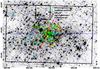 |
Fig. 1 Field of view and spatial distribution of early-type stars in the MW nuclear star cluster. The black box shows the KMOS 64.̋9 × 43.̋3 field of view, i.e. 2.51 × 1.68 pc, the small square in the upper middle was not observed due to the inactive IFU 13. Blue lines are the equatorial coordinate grid with a spacing of 10′′. The dashed blue horizontal line denotes the orientation of the Galactic plane. The black cross shows the position of Sgr A*. The underlying image is from HST/NICMOS (Dong et al. 2011), aligned along Galactic coordinates. Yellow diamond symbols denote confirmed Wolf-Rayet (WR) and emission-line stars, cyan squares are stars with featureless spectra, green circles denote O/B stars. Red ×-symbols indicate new young star candidates, blue plus-symbols probable foreground stars. The red line denotes the line of nodes of the clockwise-rotating disk of young stars. |
2.2. Data reduction
For data reduction we used the KMOS pipeline Software Package for Astronomical Reduction with KMOS (SPARK, Davies et al. 2013) in ESO Recipe Execution Tool (EsoRex). This package contains routines for processing dark frames, flat field exposures, arc frames obtained using argon and neon arc lamps, and standard star exposures. For the telluric spectra we used an IDL routine that removes the Br γ absorption line from each telluric spectrum. The routine fits the Br γ line with a Lorentz profile and subtracts the fit from the telluric spectrum. It also divides the telluric spectrum by a blackbody spectrum to remove the stellar continuum.
We reduced both science and sky exposures by applying the following steps: flat fielding, wavelength calibration, cube construction, telluric correction, and spatial illumination correction (using flat-field frames). The four sky exposures were average combined to a master sky, which we subtracted from the object cubes. We used the method described by Davies (2007), in which the sky cube is scaled to the object cube based on OH line strengths before subtraction. Then we removed the cosmic rays from each object cube with a 3D version of L.A. Cosmic (van Dokkum 2001) provided by Davies et al. (2013).
We extracted the spectra from the 736 data cubes using PampelMuse, a software package written by Kamann et al. (2013). PampelMuse was designed for extracting spectra from IFU observations of crowded stellar fields and enables clean extraction of stars even when their separation is smaller than the seeing. The program requires an accurate star catalogue. We used the catalogue provided by Schödel et al. (2010, and in prep.), which was obtained from NACO and HAWK-I observations. We ran PampelMuse separately for every IFU because the astrometry of a mosaic cube is not accurate enough and because the point-spread function (PSF) of the observations varies in time. As a consequence, the PSF in a mosaic varies between the individual 16 dither positions.
Within PampelMuse, the routine initfit uses the source list and produces a simulated image with the spatial resolution of KMOS. This image is then used as a first guess for the position of the stars in the data cubes. Since the PSF varies with wavelength, cubefit runs the PSF-fitting for each layer of the data cube. We restricted the PSF to a circular shape. This means that the PSF is defined by two variables, the FWHM and the β-parameter of the Moffat profile. The PSF variables, the coordinates, and the flux were fitted iteratively and for each layer of the data cube in the wavelength interval of [2.02−2.42 μm]. We excluded wavelength regions with prominent gas emission lines (e.g. H2, Br γ, He) from the fit.
The coordinates and the PSF vary only smoothly with wavelength, and the routine polyfit fits a 1D polynomial to the coordinate and PSF parameters as a function of wavelength. The goodness of the PSF fit depends on the number of bright stars in the IFU. For IFUs without bright stars in the field of view we used the PSF that was determined from IFUs with bright stars in the FOV. However, the PSF varies in time. Therefore we inspected the PSF fits for the 23 data cubes, where each data cube corresponds to a specific IFU. We did this separately for each exposure and selected the best PSF fits per exposure. We combined the best FWHM and best β of one exposure to a mean FWHM and mean β, both as a function of wavelength. The FWHM lies between twoto three pixels for the 32 exposures because the seeing also changed from 0.7′′ to 1.3′′ during the night. With the knowledge of the PSF of each exposure and the star coordinates, the routine cubefit was run again to determine the flux for each star on all layers of the data cubes.
After extracting background-subtracted spectra with PampelMuse, we shifted each spectrum to the local standard of rest. PampelMuse extracted ~12 000 spectra of more than 4000 different stars with KS< 17 mag in the KMOS field of view. We discarded all spectra with a signal-to-noise ratio (S/N) below 10 or negative flux, leaving ~3000 spectra. The S/N for each extracted spectrum was calculated by PampelMuse with Eq. (16) of Kamann et al. (2013). We combined the two spectra of each star from the two exposures. For ~180 stars we had even more than two spectra from the two mosaics, since PampelMuse also extracted spectra from stars that were centred outside of the field of view of the IFU. We combined the spectra with the best S/N to one spectrum per star by taking a noise-weighted mean. The S/N between the individual exposures typically differed by less than 10. We obtained spectra for more than 1000 individual stars with a formal total S/N> 10.
We also constructed a mosaic using the data cubes from all 32 exposures. This mosaic extends over 64.̋9 × 43.̋3, with a gap for the inactive IFU 13. To determine the astrometry of the mosaic, we used the 1.9 μm image of the HST/NICMOS Paschen-α Survey of the Galactic centre (Wang et al. 2010; Dong et al. 2011) as a reference. This image has a pixel scale of 0.̋1/pixel. We collapsed the KMOS mosaic data cube to an image and rebinned it to the HST pixel scale. The two images were iteratively cross correlated. Although the two images cover different wavelength regions, a large enough number of stars is detected in both images to line the frames up. Finally, we applied a correction to the local standard of rest. This mosaic data cube was used to measure the gas emission lines of the minispiral and circumnuclear ring.
3. Data analysis
3.1. Photometry
To be able to determine the spectral classes and colours of the stars, we complemented our spectroscopic data set with photometric measurements. Schödel et al. (2010, and in prep.) observed the MW nuclear star cluster with NACO and HAWK-I and constructed a star catalogue. This catalogue provides J (HAWK-I), H, and KS (HAWKI-I and NACO) photometry. The NACO catalogue extends over the central ~40′′× 40′′, HAWK-I data were used for regions farther out.
The brightest stars are saturated in the HAWK-I and NACO images, and we complemented our photometry with other star catalogues. We used photometry from the SIRIUS catalogue (Nishiyama et al. 2006) for eight stars, and for three further bright stars without HAWK-I, NACO or SIRIUS photometry, we used photometry form the 2MASS catalogue (Skrutskie et al. 2006). For almost 1000 stars we have the JHKS photometry from either NACO/HAWK-I, SIRIUS or 2MASS, for a further 100 stars we only have HKs photometry. For two stars we have no KS photometry, but JH photometry.
To obtain clean photometry, we corrected for interstellar extinction. In the Galactic centre, extinction varies on arcsecond scales (e.g. Scoville et al. 2003; Schödel et al. 2010; Fritz et al. 2011). The typical extinction values are about 2.5 mag in the KS-band, 4.5 mag in the H-band, and more than 7 mag in the J-band. We used the extinction map and the extinction law derived from Schödel et al. (2010)1 for the extinction correction of the photometry. About 350 (~30%) of the stars are outside the field of view of the extinction map. For these we assumed that the extinction is the mean value of the extinction map AKS = 2.70 mag.
The extinction map was created after excluding foreground stars. Therefore, any foreground star will be strongly over-corrected to very negative colours. The intrinsic colours of cluster members are in a very narrow range of about −0.13 mag < (H−KS) < 0.38 mag (Schödel et al. 2010, 2014b; Do et al. 2013; Cox 2000, Table 7.6, and 7.8). We used this knowledge to identify foreground stars. Stars with a bluer extinction-corrected (H−KS)0 colour than the intrinsic colour are foreground stars. To account for uncertainties in the extinction correction, we used a larger colour interval and classified a foreground star when the extinction-corrected (H−KS)0 colour was less than −0.5 mag.
Identifying background stars is less obvious. Very red stars may not be background stars, but be embedded in local dust features or have dusty envelopes. Viehmann et al. (2006) showed that several red sources in the Galactic centre are not background stars, but bow-shock sources. For red sources we have to consider the spectral type and the surroundings of the star to decide whether it is locally embedded or a background star.
3.2. Completeness
It is important to know how complete our spectroscopic data set is up to a given magnitude. Completeness is influenced by various factors, for example the depth of the observation, the spatial resolution, but also the stellar number density of the observed field. In a dense environment, crowding becomes stronger, and fewer faint stars can be detected.
We used the photometric catalogue by Schödel et al. (2010, and in prep.) to extract the stars, which means that our spectroscopic data set can at best be as complete as the photometric catalogue. Our data have a lower spatial resolution than the images used to produce the photometric catalogue, and therefore the completeness of our data set must be lower. The photometric catalogue contains ≳6000 stars in the KMOS field of view. PampelMuse extracted spectra from more than 4000 stars with KS< 17 mag. Only ~1000 of these have a spectrum with a S/N greater than 10. We determined the completeness of the spectroscopic data set by comparing our data set with the photometric catalogue in different magnitude bins. We assumed that the photometric catalogue is complete to 100% up to KS = 15 mag, at least at a projected distance p> 10′′ from Sgr A*.
The effect of crowding is illustrated in Fig. 2.
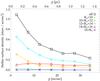 |
Fig. 2 Number density profile of the spectroscopic data set in different magnitude bins. |
We plot the number density profile of our spectroscopic data set as a function of the projected distance p to Sgr A* in different magnitude bins. Most of the stars are in the magnitude bin of 12 ≤ KS ≤ 14. The number density of bright stars with 10 ≤ KS ≤ 14 decreases with increasing radius in the central 10′′, while the number density of faint stars in the magnitude bin 14 ≤ KS ≤ 16 is nearly constant in the same radial range and even slightly increases.
The reason for this is crowding: There are more bright stars in the centre of the cluster, and they outshine the faint stars. Therefore we miss more faint stars in the centre than farther out. This effect was shown in previous studies (e.g. Schödel et al. 2007; Do et al. 2009; Bartko et al. 2010).
Completeness limits of the spectroscopic data set for different radial bins.
As a result of the higher crowding in the centre, the completeness limits depend on the distance from the centre. For this reason we determined the completeness separately for stars located within p< 5″ from Sgr A*, stars with 5″ ≤ p< 10′′, and stars beyond 10′′. The spectroscopic completeness was then estimated by comparing the number of stars as a function of magnitude N(KS) in the spectroscopic data set with the total number of stars from the photometric catalogue. We calculated the fraction of stars that are missing in the spectroscopic data set for different magnitude bins to correct our number density results by that fraction. To derive the fraction of missing stars, we binned the stars in magnitude bins of ΔKS. We varied the size of the magnitude bins to test the effect of the magnitude binning. We tried ΔKS = 0.7 mag, ΔKS = 0.5 mag, and ΔKS = 0.3 mag. The difference gives the uncertainties of the completeness limits. We list our 80% and 50% completeness limiting magnitudes in Table 1 for the three different radial bins. At greater distances, the completeness limits are shifted to fainter stars than in the centre as a result of crowding. The completeness limits did not vary beyond their uncertainty when we chose slightly different radial bins.
We investigated the effect of source confusion on our ability to classify stars. We conclude that crowding only has a minor effect on our completeness limit, and the S/N degradation does not severely affect our ability to classify stars brighter than our completeness limit.
3.3. Spectral identification of late- and early-type stars
We visually investigated the spectra and classified the stars into three categories: (a) late-type stars; (b) early-type stars; and (c) uncertain type. Late-type stars are rather cool and have CO absorption lines. Most of them are of old to intermediate age (Pfuhl et al. 2011), although there are exceptions such as the red supergiant IRS 7, which is only ~7 Myr old (Carr et al. 2000). Late-type stars are in the majority with ~990 stars. They will be analysed in detail in Feldmeier-Krause et al. (in prep.).
Early-type stars can be separated into emission-line stars, O/B stars, and featureless spectra. The data set contains 29 stars with emission lines, 23 of which are Wolf-Rayet (WR) stars and six stars have narrow emission lines (see Sect. 4.2.3). The O/B star spectra have no CO lines but rather He and/or H (Br γ) absorption lines. Our data set contains 76 O/B stars (see Sect. 4.1). A further nine stars have featureless spectra without strong absorption or emission features, but strongly increasing continuum (see Sect. 4.3). They are associated with bow shocks. The remaining 40 spectra are in category (c) of uncertain type, mostly because the S/N was too low or because the spectra are contaminated by the light of nearby brighter stars.
Figure 3 shows a colour-magnitude diagram (CMD) using H and KS after extinction correction. The location of these stars is also indicated in Fig. 1 with the same colour coding. We would like to point out that almost all WR stars are redder than the O/B stars. This is because they have evolved off the main sequence and may be producing dust. Therefore, the observed mean position of the WR stars on the red side of the CMD supports our stellar classification and the accuracy of the CMD.
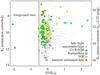 |
Fig. 3 Colour–magnitude diagram of the stars within the KMOS field of view with extracted spectra and H and KS photometry, after extinction correction. Stars with colours −0.5 mag are most likely foreground stars (left of the vertical line). Different symbols and colours denote different types of stars. Yellow circles denote emission-line/WR stars, cyan squares are sources with featureless spectra, green triangles are O/B type stars, grey dots are late-type stars, black plus-signs are stars of uncertain type. The right y-axis denotes the KS magnitude after extinction correction, with a mean extinction of AKS = 2.70 mag. |
3.4. Deriving stellar kinematics
Stellar kinematics are useful to study the origin of the early-type stars. In this section we describe our routine to fit the radial velocities of O/B stars.
The broad lines of the Wolf-Rayet stars make it difficult to determine their radial velocities. The lines are mostly a combination of several blended lines, and the stars have fast winds and outflows. For the featureless sources no spectral lines can be fitted. For the O/B stars we used thepenalized pixel-fitting (pPXF) routine to fit the Br γ and He lines (Cappellari & Emsellem 2004). We used template spectra from three different libraries: Wallace & Hinkle (1996), Hanson et al. (2005), and KMOS B-main-sequence stars. The KMOS B-main-sequence stars were observed in our program as telluric standard stars. From Hanson et al. (2005) we only used the O/B stars that were observed with ISAAC/VLT (R ~ 8000). We measured the radial velocities of the O/B templates by fitting the Br γ line and shifted the templates to the rest wavelength. The high-resolution templates were convolved with a Gaussian to match the spectral resolution of the KMOS data. Then we ran pPXF on our data.
The uncertainty of the radial velocity was measured using Monte Carlo simulations. We added random noise to the spectra and fitted the radial velocities in 100 runs. The standard deviation of the 100 measurements was our uncertainty. The results are listed in Table B.3 and are analysed in Sect. 4.5. The wavelength region of the He I and Br γ absorption lines also shows He I and Br γ emission from ionised gas (see Sect. 4.2.1). The program PampelMuse subtracts the background when extracting the stellar spectra, but the surrounding gas emission increases the noise in this wavelength region. This induces high uncertainties in our radial velocity measurements. For this reason, the median value of the radial velocity uncertainty is σmedian ≈ 60 km s-1. We compared our radial velocity measurements with the data of Bartko et al. (2009) and Yelda et al. (2014). There are nine stars with independent radial velocity measurements from this work and the previous studies. Using these stars, we can estimate the so-called true external σ of our measurement, meaning that we can test whether we over- or underestimate the uncertainties. The procedure was described by Reijns et al. (2006). First, we measured the mean velocity offsets ⟨ vi−vj ⟩ (i = 1,2,3;j = 2,3,1) between each pair of the three studies for the overlap stars and the respective standard deviation  . Because
  , we can calculate the true σvi (i = 1,2,3) from the three measurements of .
A comparison of the external error σext with the mean error σmean of the individual radial velocity measurements indicates whether we over- or underestimate the uncertainty. The external error σext = 45 km s-1 for our radial velocities is smaller than the mean error σmean of the nine overlap stars. σext is approximately 0.7 times the mean error σmean. Of the nine stars with three independent radial velocity measurements, five stars in our data set have a high S/N> 56 (Id 109, 205, 294, 331, 372), but four stars (Id 707, 1123, 1238, 2233) have a low S/N (<30). The velocities of three of these four stars with low S/N agree with the measurement of Bartko et al. (2009) or Yelda et al. (2014) within the uncertainties. However, we consider the radial velocity measurements of the five stars with the higher S/N more reliable. The external error calculated from the five stars with high S/N is σext = 27 km s-1. This is 0.8 times the mean error σmean, thus our errors appear to be accurate to within 20%. Although nine independent radial velocity measurements are not enough for an accurate determination of σext, our analysis indicates that we do not underestimate the radial velocity errors.
4. Results
Here we first present the O/B type stars, and we derive their masses from the photometry. We obtain maps of the emission line flux that is generated by the minispiral and the circumnuclear ring. For stars with narrow emission lines and Wolf-Rayet stars we show spectra and the spectral classification, followed by the spectra of featureless sources. We finally present the spatial distribution of the early-type stars. We also investigate the O/B star kinematics and stellar orbits.
4.1. O/B type stars
4.1.1. Identifying O/B stars
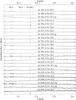 |
Fig. 4 Spectra of the newly identified O/B type stars. The fluxes are normalised and an offset is added to the flux. The spectra are not shifted to rest wavelength. The numbers denote the identification numbers of the stars as listed in Tables B.1−B.3. We also show the S/N and denote probable foreground stars with “fg”. |
O/B-stars have effective temperatures of Teff> 10 000 K (e.g. Martins et al. 2005; Crowther et al. 2006). The most prominent lines in O/B giant K-band spectra are the He I (2.058 μm, 2.113 μm and ~2.164 μm), H I (4-7) Br γ (2.166 μm), and He II (2.1885 μm) lines (Hanson et al. 2005). The 2.113 μm complex is also partly generated by N III. These lines appear mostly in absorption, but can also be in emission or absent, depending on the spectral type (Morris et al. 1996).
Previous studies found ~100 O/B supergiants, giants, and main-sequence stars in the innermost parsec of the Galaxy (e.g. Paumard et al. 2006; Bartko et al. 2009; Do et al. 2013; Støstad et al. 2015). Our spectroscopic data set contains 76 O/B stars, 52 of which were reported in previous spectroscopic studies, but 24 sources appear not to have been identified before, due primarily to the wider field of view of our observations relative to previous spectroscopic studies.
The spectra of the newly identified O/B stars are shown in Fig. 4. Five of them are probably foreground stars, as they have very blue colours (Id 436, 663, 1104, 3308, and 3339, (H−KS)0 = −2.04,−0.53,−0.52,−0.50, and −1.92 mag). For one of the O/B stars (Id 982) we had to assume a mean extinction value of AKS = 2.70 mag because this star is beyond the field of view of the extinction map of Schödel et al. (2010). This means there is a large uncertainty in the star’s colour of (H−KS)0 = 0.04 mag. If the local extinction is higher than the assumed mean extinction value of AKS = 2.70 mag, this could mean that this star also is a foreground star. For the star Id 2048 we have no colour information and cannot determine whether this star is a foreground star.
We list our sample of O/B-type stars in Table B.1. This table provides the star Id, right ascension RA, declination Dec (in equatorial coordinates), the offset coordinates ΔRA and ΔDec with respect to Sgr A*, the magnitude KS, remarks on the star colour, the star name and type (if available), a note to the respective reference, and the S/N.
The O/B-type stars were identified by inspecting the spectra of all stars in our data set. To verify our visual classification, we measured the equivalent widths (EW) of the 12CO(2,0) line at 2.2935 μm, and the Na I doublet at 2.2062 μm and 2.2090 μm. We used the definitions of band and continuum from Frogel et al. (2001). For the late-type stars we obtain a mean value of EWCO,LT = 18.30 (EWNa,LT = 4.60) with a standard deviation of σCO,LT = 5.20 (σNa,LT = 2.13). The mean uncertainty is only ΔEWCO,LT = 0.39 (ΔEWNa,LT = 0.25). For the O/B stars, the equivalent widths for CO and Na are lower, with a mean value of EWCO,O/B = −0.76 and σCO,O/B = 3.25 (EWNa,O/B = 0.47 and σNa,O/B = 1.75). This means that the equivalent width of the CO line of O/B stars is on average more than 3.67σ smaller than for late-type stars, and the equivalent width of Na is ~1.97σ smaller. We list the equivalent widths of CO and Na for the O/B stars in Table B.2.
O/B giants and supergiants have observed magnitudes of KS=11−13 mag at the Galactic centre, while O/B main-sequence stars have KS = 13−15 mag (Eisenhauer et al. 2005; Paumard et al. 2006). To estimate the luminosity class of the O/B stars in our sample, we corrected the KS magnitude using the extinction map provided by Schödel et al. (2010) and added a mean extinction of AKs = 2.70 mag to the KS magnitude. We chose AKs = 2.70 mag since this is the mean value of AKs from Schödel et al. (2010) in our field of view. The resulting values are given in Table B.1 (see also the right y-axis in Fig. 3). With this rough magnitude cut, we estimate that about 70% of the O/B stars in our data set are giants or supergiants, and 30% are main-sequence stars.
4.1.2. Mass estimates and dust extinction
To determine the spectral type of O/B stars in the K-band, the data quality has to be very high. The He I line at 2.058 μm is in a region of high telluric absorption and low S/N. The minispiral emission increases the noise at 2.058 μm and 2.166 μm. Since the gas emission is spatially highly variable, the background subtraction is imperfect. But even without these difficulties, a spectral classification is complicated. Hanson et al. (2005) collected K-band spectra of O and early-B stars of known spectral type. They found that for a determination of Teff and log g, the spectral resolution should be R ≈ 5000 or higher. Furthermore, a S/N> 100 is desirable. For the stars in our data set, these conditions are not fulfilled. Therefore we cannot place more constraints on the spectral types of our O/B star sample.
Nevertheless, we can estimate the mass of the O/B stars under some assumptions from the photometry. The intrinsic colour of O/B stars is in a very narrow range close to (H−KS)0 ≈ −0.1 mag (Cox 2000, Tables 7.6, and 7.8). Therefore the wide spread of the O/B stars over ~1 mag on the CMD (Fig. 3) is mostly due to imperfect extinction correction. For the extinction correction we used the extinction map of Schödel et al. (2010). It was derived by averaging over several stars and is therefore only an approximation to the real local extinction. However, because we spectroscopically selected the stars and all O/B stars have intrinsic colours (H−KS)0 ≈ −0.1 mag, we can use the photometric colours to obtain independent extinction estimates. We assumed an extinction law of Aλ ∝ λ− α to calculate the true extinction for each single O/B star and its true magnitude KS,0. We used the extinction law coefficient of α = 2.21 (Schödel et al. 2010). The results for KS,0 and AKS are listed in Cols. 4 and 5 of Table B.2 for the 73 O/B stars with H and KS photometry. The uncertainty σKs,0 contains the propagated error of the measured photometry σH and σKS, the error of the true intrinsic colour σH−KS, the extinction-law coefficient uncertainty σα, and the Galactocentric distance uncertainty σR0.
The derived extinction values AKS range from 0.42 mag for probable foreground stars to 3.06 mag. The median extinction value of O/B stars that are not flagged as foreground stars is 2.48 mag with a standard deviation of 0.22 mag. The extinction derived from the extinction map is mostly higher, with a median of AKS = 2.63 mag and a standard deviation of 0.15 mag. We plot the extinction derived from the intrinsic colours against the extinction from the extinction map of Schödel et al. (2010) in Fig. 5. For the two stars Id 436 and 3339 it is obvious that they are foreground stars, the extinction derived from the intrinsic colour is lower by more than 2 mag than AKS from the extinction map. We also classified the three stars Id 663, 1104, and 3308 as foreground stars. With the large uncertainty of the extinction, these stars might be cluster member stars.
There appears to be a systematic offset between the extinction: AKS derived from intrinsic colours is mostly lower by ~0.2 mag than the value of AKS from the extinction map. We varied different input parameters to test their effect on our result of AKS. A lower value of (H−KS)0 than −0.1 mag is unlikely. However, when we changed the extinction law coefficient α from 2.21 (Schödel et al. 2010) to 2.1, the offset of 0.2 mag disappeared. Previous studies measured α in the range of 2.0 to 2.64 (Gosling et al. 2009; Stead & Hoare 2009; Nishiyama et al. 2009; Schödel et al. 2010). The value of α has the largest uncertainty and can therefore alone account for the offset.
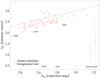 |
Fig. 5 Comparison of the extinction AKS in magnitudes derived from the intrinsic colour with the extinction from the extinction map of Schödel et al. (2010) for O/B stars. The black line denotes the 1:1 line, blue squares are foreground stars, red triangles are cluster member stars. Typical error bars are shown in the lower right corner. |
We also used isochrones to estimate the stellar mass given the position of the star in the CMD. We used the isochrones of Bressan et al. (2012), Chen et al. (2014) and Tang et al. (2014) downloaded at2 with solar metallicity. Ramírez et al. (2000) found that the iron abundance Fe/H of the Galactic centre stars is roughly solar. However, the α-element abundance is super-solar (Cunha et al. 2007; Martins et al. 2008). Paumard et al. (2006) and Lu et al. (2013) showed that the young population in the Galactic centre is 3−8 Myr old. We used isochrones in this age interval with a spacing of Δ(log (age/ yr)) = 0.01. The isochrones are for 2MASS photometry, therefore we shifted the colours to our ESO photometry using the equations given by Carpenter (2001, 2003 version at3.
For the O/B stars in our data set we computed the likelihood ℒ of (H−KS)0 = (H−Ks)iso and KS,0 = KS,iso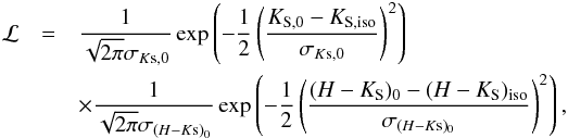 where (H−Ks)iso and KS,iso are the isochrone points from all isochrones in our age interval. To each isochrone point there is a corresponding stellar mass ℳ. Because we used various isochrones, there can be different stellar mass values for the same value of (H−Ks)iso and KS,iso. We have a distribution of stellar masses, and we used the likelihood to calculate the probability mass function of the stellar mass for each O/B star separately. In Table B.2 we list the median mass of each star in the probability function (column ℳ), the uncertainties are derived from the 0.16 and 0.84 percentiles. Figure 6 shows the cumulative mass distribution of star Id 617 as an example.
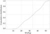 |
Fig. 6 Cumulative mass distribution of star Id 617. The horizontal lines denote 0.16, 0.5, and 0.86 percentiles, the vertical lines denote the corresponding masses. We derived a mass of |

The masses of our O/B star sample range from 43 M⊙ for the brightest stars to only 7 M⊙ for a probable foreground star. When we used isochrones with a slightly higher metallicity, we obtained lower stellar masses in most cases. However, the results agree within their uncertainties.
We estimated the total mass of the young star cluster with some assumptions. In Sect. 3.1 we have shown that the 80% completeness limit is at KS ≈ 13.2 mag. When we consider only O/B stars with KS ≤ 13.2 mag and with ℳ ≥ 30 M⊙, the mass function is approximately complete. The initial mass function (IMF) of young stars in the Galactic centre is top-heavy (Bartko et al. 2010; Lu et al. 2013). We fitted the IMF dN/ dm = A × m− α to the observed mass function in the mass interval [30 M⊙;43 M⊙], where we have 51 stars. We used the software mpfit (Markwardt 2009) to fit the coefficient A and use α values from the literature. We refrained from fitting α. The covered mass interval and the number of stars are too small to constrain the shape of the IMF. Then we integrated the IMF from ℳ = [1 M⊙;ℳmax] to obtain the total mass of the young star cluster. As our mass function contains only O/B stars and no emission-line stars, which are also young and in the same mass interval, we derived only a lower limit for the young star cluster mass.
Assuming an IMF with α = 1.7 (Lu et al. 2013) and ℳmax = 150 M⊙, we obtain 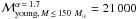 M⊙, and with α = 0.45 (Bartko et al. 2010), we obtain
 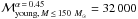 M⊙. With an upper integration limit of ℳmax = 80 M⊙, the young cluster mass is
  M⊙ for α = 1.7 and
 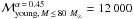 M⊙ for α = 0.45. We thus give ℳtotal,young ~ 12 000 M⊙ as a lower limit for the mass of the young star cluster. When we consider the lower mass limits of the stars, the total mass is decreased to
 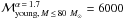 M⊙ (
M⊙ ( M⊙). The binning uncertainty is also of the order ~3000 M⊙.
4.2. Emission line sources
There are three sources of emission lines in the Galactic centre: (a) Extended ionised gas streamers, the so-called minispiral, or Sgr A East; (b) molecular gas; and (c) emission-line stars, which mostly are WR stars.
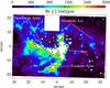 |
Fig. 7 Emission line map of Br γ gas at 2.1661 μm of the full KMOS mosaic. The axes show the distance from Sgr A* (red plus sign) in Galactic coordinates. Black crosses with cyan surrounding square symbols denote the positions of the sources with featureless spectra (see Sect. 4.3). The flux of Br γ emission is not saturated, but the scaling was set low in order to show the fainter, extended structure of the minispiral. |
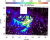 |
Fig. 8 Same as Fig. 7 for He I gas at 2.0587 μm. The black plus sign denotes the position of Sgr A*. The He I emission line is weaker than the Br γ line. Black crosses with yellow surrounding square symbols denote the positions of the emission-line stars (see Sect. 4.2.3). The He I line flux is not saturated in the data, but we set the scaling in this image low in order to show the extended structure of the minispiral. |
4.2.1. Ionised gas streamers
The gas streamers of the minispiral can be seen in our data in the H I (4−7) Br γ 2.166 μm and He I 2.058 μm (2s1S–2p ) lines. We fitted Gaussians to the H I Br γ and He I 2.058 μm emission lines using the KMOS mosaic. The resulting flux maps are shown in Fig. 7 for Br γ and in Fig. 8 for He I emission. The images are oriented in the Galactic coordinate system and are centred on Sgr A*, which is shown as a red or black cross. We chose the applied flux scaling in the Figs. 7 and 8 to show the extended minispiral structure, but the flux of the emission lines is not saturated in the data. The H I Br γ emission is stronger than the He I emission, therefore the He I map is noisier.
The gas emission is very bright and complicates the measurement of equivalent widths of the He I and H I Br γ absorption features of O/B-type stars. Since the gas emission is also highly variable on small spatial scales, we refrained from modelling the gas emission. PampelMuse subtracted the surrounding background from the spectra, but residuals remain in our data. Subtracting the gas emission close to the star can be complicated even for high-angular resolution data (see Paumard et al. 2006). However, as the gas emission lines are very narrow compared to emission lines from Wolf-Rayet stars and because most emission-line stars have additional C or N lines, we can distinguish between the different emission line sources.
4.2.2. Molecular gas
The molecular gas in the Galactic centre is concentrated in a circumnuclear ring (CNR). This clumpy gas ring extends over a projected distance of ~1.6 to 7 pc (41′′−3′, e.g. Yusef-Zadeh et al. 2001; Lee et al. 2008; Smith & Wardle 2014) and rotates with ~110 km s-1 (Christopher et al. 2005; Feldmeier et al. 2014). The gas ring consists of two prominent symmetric lobes north-east and south-west of Sgr A*.
Our data set maps only the inner edge of the circumnuclear ring. We fitted Gaussians to the H2 emission line at 2.1218 μm (1–0 S(1)) using the KMOS mosaic. Figure 9 shows the H2 flux map in the Galactic coordinate system. There are several gas streamers and clumpy structures within the projected distance of the circumnuclear ring.
Emission-line and Wolf-Rayet stars.
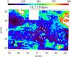 |
Fig. 9 Same as Fig. 7 for H2 gas at 2.1218 μm. The red plus sign denotes the position of Sgr A*. The H2 line flux is not saturated in the data, but we set the scaling in this image low in order to show the extended structure of the gas. |
4.2.3. Emission-line stars: spectral classification
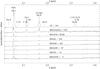 |
Fig. 10 Spectra of stars with narrow emission lines and Wolf-Rayet stars. The lower six spectra are Ofpe/WN9 stars with narrow emission lines (FWHM ~ 200 km s-1). Fluxes are normalised and an offset is added to the flux. The spectra are not shifted to rest wavelength. The narrow emission line in the 2.167 μm emission line of spectrum Id 1237 is a residual of poorly subtracted minispiral emission. |
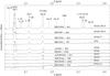 |
Fig. 11 Spectra of Wolf-Rayet stars of type WN and WN/WC, ordered by increasing WN-type from bottom to top. The fluxes are normalised and an offset is added to the flux. The spectra are not shifted to rest wavelength. |
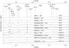 |
Fig. 12 Spectra of Wolf-Rayet stars of type WC. The classification from Paumard et al. (2006, PGM2006) is written for all spectra. The narrow emission line at 2.167 μm of spectrum Id 784 is a residual of the subtracted minispiral emission. The fluxes are normalised and an offset is added to the flux. The spectra are not shifted to rest wavelength. |
Stars with a He I 2.058 μm emission line can belong to many different types such as WR stars, intermediate types such as Ofpe/WN9 (O-type spectra with additional H, He, and N emission lines, and other peculiarities), and luminous blue variable (LBV) stars. Paumard et al. (2001) suggested two classes of He I 2.058 μm emission-line stars in the Galactic centre: Stars with narrow emission lines (FWHM ~ 200 km s-1) and stars with very broad emission lines (FWHM ~ 1000 km s-1). Paumard et al. (2001) roughly sorted narrow-line stars into LBV-type stars, with temperatures of 10 000−20 000 K, and broad-line stars to WR-type stars, with higher temperatures of >30 000 K. In broad-line star spectra the lines have a higher peak value above the continuum than in narrow-line star spectra.
Wolf-Rayet stars are evolved, massive stars (>20 M⊙ while on the main sequence, Sander et al. 2012). Their spectra show strong emission lines because these stars are losing mass. Figer et al. (1997) provided a list of WR emission lines in the K-band; among them the He I, He II, H I, N III, C III, and C IV transitions. WR stars can be sorted into WN and in WC types. WN-type spectra are dominated by nitrogen lines and WC-type spectra are dominated by carbon and oxygen.
We have 29 spectra with a He I 2.058 μm emission line/WR stars. These stars are already known, for instance from Krabbe et al. (1995), Blum et al. (2003) and Paumard et al. (2006). We list these stars in Table 2, and their spatial distribution is shown in Fig. 1 with yellow symbols. The spectra are shown in Figs. 10−12. In some spectra the residual from the minispiral gas emission after the subtraction is still visible, for example in Id. 1237/IRS 7E2 (ESE) at ~2.167 μm. The brightest WR stars are also visible in the emission line maps in Figs. 7 and 8 as bright point sources. As a result of their large FWHM, the emission lines are blends of several lines. Therefore radial velocity measurements of WR stars are highly uncertain with our data. Tanner et al. (2006) obtained high-resolution spectra and measured the radial velocities of emission lines stars in the Galactic centre.
Paumard et al. (2006) listed eight stars in their Table 2 as Ofpe/WN9 stars because they showed narrow emission lines and a He I complex at 2.113 μm. The KMOS spectra of these stars are shown in Fig. 10. All spectra have P Cygni profiles at 2.058 μm, at the He I line. This indicates that these stars are a source of strong stellar winds (~200 km s-1). However, two of the stars (Id 144/AF and Id 1237/IRS 7E2 (ESE)) look different in our data from the other Ofpe/WN9 stars. They have significantly broader lines, with FWHM ~ 700 km s-1 instead of ~200 km s-1. The 2.113 μm feature is mostly in emission and not in absorption, in contrast to the other six as Ofpe/WN9 identified stars. Furthermore, a feature at He II 2.1891 μm appears in emission. Figer et al. (1997) showed that the ratio between the 2.1891 μm feature and the 2.11 μm feature is strongly correlated with subtypes for WN stars and increases with earlier subtype. This 2.1891 μm feature is also present in the other WN stars of our data (see Fig. 11). Therefore we conclude that the stars Id 144/AF and Id 1237/IRS 7E2 (ESE) are not Ofpe/WN9 stars but are hotter stars, such as WN8 or WN9. Tanner et al. (2006) also classified star AF (Id 1206) as a broad emission-line star.
The spectra of stars classified as WN stars in Paumard et al. (2006) are shown in Fig. 11. WN stars can be separated into an early (WN2 to WN6) and a late group (WN6 to WN9). The only early WN star in our data, Id 574/IRS 16SE2, is a WN5/6 star (Horrobin et al. 2004). The spectrum of Id 155/IRS 13E2 is classified as that of an WN star by Paumard et al. (2006) without further specification. We find that this spectrum resembles the late WN8 spectra of Id 452/AFNW and Id 1354/IRS 9W. Stars Id 784/WR101da and Id 1494/IRS34 NW were classified as WN7 stars. Their spectra have only weak emission lines, for example at 2.189 μm (He II) and 2.347 μm (He II).
Star Id 491/IRS 15SW was classified as a transition-type WN8/WC9 star by Paumard et al. (2006). In addition to the aforementioned He I and He II emission lines, the spectrum shows the C IV doublet at 2.0796 and 2.0842 μm, and C III at ~2.325 μm in emission. These features are much weaker than the He and H lines. The spectrum of Id 666/IRS 7SW has the same C IV and C III lines, although it was classified as WN8 by Paumard et al. (2006). Therefore we suggest that Id 666/IRS 7SW is a WN/WC transition-type star like Id 491/IRS 15SW.
WC stars have C III and C IV emission lines that are about as strong as the He lines. Figure 12 shows the spectra of WC stars in our data set. The classifications are adopted from Paumard et al. (2006). We find that for stars Id 185/IRS 29N, Id 283/IRS 34, Id 303, and Id 638/IRS 29NE1 the emission lines are rather weak. This cannot be caused by the S/N, which is higher than 55 for all of the four spectra. The continua of these four spectra show a steep rise with wavelength, and these stars are also very red ((H−KS)0> 0.54 mag). This suggests that these stars are embedded in dust (Geballe et al. 2006). The continuum emission from the surrounding dust dilutes the stellar spectral lines (for a discussion see Appendix A).
In summary, we confirm that 29 stars are emission-line stars. We classify the stars Id 144/AF and Id 1237/IRS 7E2 as broad emission-line stars and the star Id 666/IRS 7SW as a WN8/WC9 star, in contrast to Paumard et al. (2006). Four of the stars (Id 185/IRS 29N, Id 283/IRS 34, Id 303, and Id 638/IRS 29NE1) have only weak emission lines, which can be explained by bright surrounding dust. Despite their red colours, we do not consider them to be background stars. We discuss these findings in Appendix A.
4.3. Featureless spectra
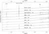 |
Fig. 13 Featureless spectra. Emission lines are due to imperfect background subtraction and caused by He I, H I, and H2 gas emission. The fluxes are normalised and an offset is added to the flux. The spectra are not shifted to rest wavelength. |
Stars with featureless spectra.
Previous studies pointed out that several sources apparently have featureless, steep K-band spectra in the Galactic centre. For example, the spectra of IRS 3 and IRS 1W show no detectable emission or absorption features (e.g. Krabbe et al. 1995; Blum et al. 2003). These sources are often extended in mid-infrared images, and it was shown that they are bow shocks. Bow shocks are caused by bright emission-line stars that either have strong winds or move through the minispiral (e.g. Tanner et al. 2005, 2006; Geballe et al. 2006; Viehmann et al. 2006; Perger et al. 2008; Buchholz et al. 2009; Sanchez-Bermudez et al. 2014).
We detected several featureless sources in our KMOS data. They are listed in Table 3, and their spectra are shown in Fig. 13. The first column of Table 3 denotes the Id, RA, and Dec from our catalogue. Most of the sources with featureless spectra are located close to the minispiral. The last column of Table 3 gives their location within the minispiral. We also indicate their positions in Fig. 7. Many of the stars are either connected with the Northern Arm (NA) or the Bar. Only star Id 247/IRS 3 is in a region of low ionised gas emission. Nevertheless, it is the most reddened of these sources.
Bow shocks arise through the interaction of the interstellar medium (like the minispiral gas) with the material expelled from mass-losing stars. The central sources of Id 161/IRS 5 and Id 25347/IRS 1W are probably WR stars (Tanner et al. 2005; Sanchez-Bermudez et al. 2014). The source Id 247/IRS 3 was classified as WC5/6 (Horrobin et al. 2004) and as an AGB star (Pott et al. 2005). The spectrum of Id 247/IRS 3 shows a broad emission bump at 2.078 μm, but this could be caused by the close WN5/6 star IRS 3E. This star is rather faint (KS = 14.1 mag), however, compared to star Id 247 (KS = 11.2 mag), and therefore the spectrum has a too low S/N and is missing from our list of WR stars.
The spectrum of Id 477/IRS 8 in our data is nearly featureless, but Geballe et al. (2006) was able to separate the spectrum of IRS 8 into the contribution of the bow shock and the actual star, IRS 8*. They showed that star IRS 8* has several weak emission and absorption lines and classified IRS 8* as O star. One star in our sample of featureless sources (Id 705) was classified as a late-type star by Perger et al. (2008).
These featureless sources are also very red in H−KS, as we show in Fig. 3. We find that of all of the sources, the spectra of Id 247/IRS 3 and Id 541/IRS 2L have the steepest continuum rise to longer wavelengths (slope m = Δflux/Δλ = 4.2 and 3.3, respectively). These sources are probably not background stars, but surrounding dust causes the reddening.
In brief, many stars with featureless spectra were either classified as young emission-line or O-type star, or their red colour and continuum shape suggest that they are young, embedded stars. Therefore we also consider these stars as young early-type stars of the MW nuclear star cluster.
4.4. Spatial distribution of early-type stars
Our wide-field study of early-type stars confirms the results of previous studies in smaller regions (e.g. Støstad et al. 2015). Young stars are mostly concentrated at p< 0.5 pc (see Fig. 1). Previous spectroscopic data sets were spatially asymmetric with respect to Sgr A* and therefore were potentially biased. For example, Do et al. (2013) observed the Galactic centre along the projected disk of young stars. Our data set is completely symmetric with respect to Sgr A* out to p = 12′′ (~0.48 pc). In the radial range to p = 21′′ (0.84 pc) we only miss a small field of 10.̋8 × 10.̋8, therefore the area is complete to 91% out to p = 21′′ (0.84 pc). The spatially nearly full coverage allows us to study the spatial distribution of early-type stars.
Figure 14 shows the cumulative number counts of our observed early-type stars and late-type stars normalised to one, as a function of projected distance p to Sgr A*. Most of the early-type stars lie within the central parsec and reach a cumulative frequency of 0.9 at p = 12′′ (0.47 pc), whereas the late-type stars are distributed throughout the entire cluster range. For this plot we did not correct for completeness. Including a completeness correction would steepen the lines in the innermost regions even more. The median projected distance to the centre is only 6.6′′ (~0.26 pc) for the early-type stars, but 19′′ (0.74 pc) for the late-type stars. We list the projected distance p to Sgr A* for the O/B stars in Table B.3. The outermost O/B star that is not a foreground star is Id 982 with p = 23.6′′ (0.92 pc). Only the featureless source Id 477/IRS 8 has a larger distance p = 29.4′′ among the early-type stars.
While we benefit from the large spatial coverage, our data set lacks the spatial resolution and the higher completeness of other studies (e.g. Bartko et al. 2010; Do et al. 2013). In Sect. 3.2 we calculated the fraction of stars that we missed in different radial and magnitude bins. We used three radial bins (p< 5″, 5″ ≤ p< 10″, and p ≥ 10″) and magnitude bins with a width of ΔKS = 0.5 mag. We corrected our number counts of early-type stars in the different magnitude and radial bins by including the fraction of missed stars. Then we computed a completeness-corrected stellar number density of bright stars with KS< 14.3. We find excellent agreement with the results of Do et al. (2013, K′< 14.3, as shown in Fig. 15. Our data set extends to larger radii beyond 10′′. There are only a few stars in this region, and the number density of bright early-type stars decreases by more than two orders of magnitude from the centre to a projected distance of p = 1 pc.
Inspection of Fig. 1 shows that the distribution of early-type stars (i.e. O/B stars, emission-line stars, and sources with featureless spectra) appears elongated, primarily along the Galactic plane. However, there is a slight misalignment of the distribution of early-type stars with respect to the Galactic plane. Most early-type stars beyond 0.5 pc (~12.8′′) are either in the Galactic north-west (NW, top right), or south-east (SE, bottom left) quadrant. We note that on larger scales the rotation axis also seems offset from the Galactic plane in a similar direction (Feldmeier et al. 2014). The early-type stars are more centrally concentrated in the north-east (NE) and south-west (SW) fields than in the SE and NW fields. The median projected distances  are
are  pc (5.0′′) and
  pc (5.8′′) in the NE and SW field, but
  pc (6.6′′) and
  pc (7.8′′) in the SE and NW fields.
To quantify a possible asymmetric distribution, we compared the number of early-type stars in the different quadrants Galactic NE, SE, SW, and NW. The centre is the position of Sgr A*. We corrected for the slightly asymmetrically covered area and compare the number of stars Nfield in different fields. Probable foreground stars were not taken into account. We find that there are about the same number of early-type stars in the NE, SE and SW fields, but ≈1.4 times more early-type stars in the NW quadrant (corresponding to more than ten stars). This is in contrast to the distribution of late-type stars, for which there are the fewest stars in the Galactic NW.
As some of the early-type stars in the central ~0.5 pc are on a disk, asymmetry is not unexpected. However, Fig. 1 shows that the line of nodes of the disk is ~60°offset from the Galactic plane. The early-type stars also appear offset from the Galactic plane, but not by as much. An important observational bias is introduced by the spatially variable extinction. This is also shown in Fig. 1. In the underlying 1.90 μm image there are some patchy regions with less flux, for instance in the SW corner of the image. We detect fewer stars in these regions and find an asymmetric spatial distribution of early-type stars. As our extinction map does not extend to this region, we cannot quantify the effect of the variable extinction. Thus we cannot conclude whether dust alone can explain the asymmetry.
4.5. Kinematics of early-type stars
The early-type stars in the Galactic centre can be distributed into different groups based on their kinematics. In the central p< 0.03 pc (~0.8′′) is the S-star cluster. This group of ≳20 stars has high orbital eccentricities e ( , Gillessen et al. 2009b). Most of the stars are B-type main-sequence stars (Ks ≳ 14 mag). These stars are mostly too faint and too crowded to be in our data set. The only exception is S2 (Id 2314), which is one of the brightest S-stars with KS = 14.1 mag (for a Table of 51 sources in the S-star cluster see Sabha et al. 2010).
At greater distances, 0.03 pc<p< 0.5 pc (0.8′′−13′′), there is a clockwise (CW) rotating disk of young stars with moderate orbital eccentricities (e ~ 0.3). This disk contains WR, O, and B stars (Yelda et al. 2014). Not all stars in this radial range lie on the disk, there is also a more isotropic off-disk population. The disk and off-disk populations are very similar and probably coeval (Paumard et al. 2006). It is not yet settled whether there is a second, counterclockwise rotating disk. To assess whether a star belongs to the disk or not and if the star is on a bound orbit, we have to know the stellar kinematics.
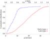 |
Fig. 14 Cumulative number counts of early-type stars (blue plus signs) and late-type stars (red crosses) as a function of projected distance p from Sgr A*, normalised to one. Foreground stars were excluded. |
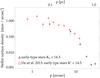 |
Fig. 15 Stellar surface density profile for all early-type stars (O/B, emission line stars, and sources with featureless spectra). We exclude possible foreground stars and apply a completeness correction (see Sect. 3.1). We consider only stars brighter than KS = 14.3. Black triangles denote this study, red squares the results of Do et al. (2013). |
We measured the radial velocities of O/B stars as described in Sect. 3.4, and Table B.3 lists the radial velocities vz of the O/B stars. When no good radial velocity measurement was possible with our spectra, we list the radial velocity of Bartko et al. (2009), Yelda et al. (2014), or an error-weighted mean of their measurements. Furthermore, we match the O/B stars of our data set with the proper motions of Yelda et al. (2014) and Schödel et al. (2009). These measurements are also listed in Table B.3 as vRA and vDec. To transfer the proper motion velocities into km s-1, we assumed a Galactocentric distance of R0 = 8 kpc.
About 20 young stars are on the CW disk (Yelda et al. 2014). The CW disk has the orbital parameters inclination i = 130° and ascending node Ω = 96° (e.g. Yelda et al. 2014; Bartko et al. 2009; Lu et al. 2009; Paumard et al. 2006). The stars on the CW disk are approaching (negative radial velocity, vz< 0) in the equatorial North-West, and receding (positive radial velocity, vz> 0) in the equatorial South-East. Based on this simple criterion, we can exclude the membership of 23 stars of our O/B star sample, 7 of which are newly identified O/B stars. We list in the second last column of Table B.3 whether vz agrees with the rotation of the CW disk or not. If the entry in the second last column of Table B.3 is 0, a membership to the CW disk is not possible according to vz, given the longitude of the ascending node Ω is 96°. If the disk is warped, as found by Bartko et al. (2009), the value of Ω would change with the distance to Sgr A*. Then the radial velocity criterion would exclude one star less.
The stellar kinematics are illustrated in Fig. 16. For 45 O/B stars we have the radial velocity and proper motions, and for 22 stars proper motions alone. The directions of the arrows denote the proper motion direction, the lengths of the arrows denote the proper motion velocity vpm assuming a distance of 8 kpc. Additionally, we overplot the kinematics of the emission-line stars with 27 radial velocities adopted from Tanner et al. (2006), and 28 proper motion measurements as slightly smaller arrows. Proper motions are taken from Yelda et al. (2014) if available, and from Schödel et al. (2009) otherwise. Because we used the disk parameters of Yelda et al. (2014) in our analysis, we give preference to the proper motions derived by this study.
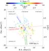 |
Fig. 16 Three-dimensional stellar kinematics of the O/B stars and emission line stars (smaller arrows). The arrows denote the proper motions, colours signify different radial velocities vz. The black cross indicates the position of Sgr A*. The coordinates show the offset to Sgr A* in equatorial coordinates, the numbers at the top and left denote absolute equatorial coordinates. The Galactic plane is plotted as a blue dashed line, and the line of nodes of the clockwise disk with Ω = 96° is shown as a red line. The green dot-dashed line illustrates the projected rotation axis of the clockwise disk. |
4.6. O/B star orbits
To identify stars on radial or tangential orbits, the angular momentum jz = xvy−yvx can be used, or as suggested by Madigan et al. (2014), jz normalised to the maximum angular momentum at projected radius p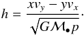 (1)x and y denote the distance to Sgr A* in equatorial coordinates, vx and vy are the proper motions in the same coordinate system, ℳ• = 4.3 × 10⁶M⊙ (Ghez et al. 2008; Gillessen et al. 2009b) is the mass of the supermassive black hole, and G is the gravitational constant.
The h-value constrains the stellar orbital eccentricity and shows whether the star is on a projected orbit that is clockwise (CW) tangential (h ~ 1) or counterclockwise tangential (h ~ −1). We also list h in Table B.3. If h is negative, this star is probably not a member of the CW disk, although the radial velocity vz may agree with the CW disk. A value of h ≈ 0 does in principle mean the star is on a radial projected orbit. But this can have different reasons: Either the star has a high orbital eccentricity (e ≳ 0.8), a highly inclined orbit (i ≳ 70°, with 90° meaning edge-on), or both. If we have both proper motion and radial velocity for a star, we can compare the magnitude of the proper motion velocity  to the total three-dimensional velocity vtot. If the proper motion velocity is much lower than the radial velocity, that is, the three-dimensional velocity vector is mainly pointing along our line of sight, the star is on a close to edge-on orbit. For example, a value of vpm/vtot ≤ 0.2 indicates a high inclination of the orbit. Then a low value of | h | tells us nothing about the eccentricity of the stellar orbit.
Twenty-four stars have | h | ≤ 0.2, suggesting a high eccentricity e, a high inclination i, or both. For 18 of these stars we have kinematics in three dimensions, thus we can infer for three stars that they have orbits with high inclination, they are marked with a footnote in Table B.3 (Id 483, 728, and 853). On the other hand, we have 11 stars with | h | ≤ 0.2, for which the ratio | vpm | /vtot ≥ 0.6 indicates a rather low inclination. Therefore the orbits of these stars have truly high eccentricities.
Although a low value of | h | does not necessarily mean a radial orbit, a value of h> 0.6 is an indication that a star is on the CW disk. Our data set contains 14 stars (~20%) with h> 0.6, for eight (~12%) of them vz also agrees with the CW disk, but for four of them it does not. Only one star of the new O/B stars is a good candidate for being on the CW disk: Id 596 has h = 0.82 and is at a distance of p = 7.35′′ (~0.3 pc) from Sgr A*.
To determine the full orbit of a star and thereby constrain the disk membership, it is also necessary to consider the distance of the star along the line of sight. Lu et al. (2009) and Yelda et al. (2014) included measurements of the plane-of-sky acceleration to constrain the stars’ line-of-sight distances to Sgr A*. To better constrain the orbital parameters, previous studies (e.g. Lu et al. 2009; Bartko et al. 2009; Yelda et al. 2014; Sanchez-Bermudez et al. 2014) computed density maps of the orbital planes and ran Monte Carlo simulations.
For one star, Id 96, the value of | h | is even higher than 1: h = −1.05. According to Madigan et al. (2014), this means the star is still on a bound orbit, as  . But it requires the semi-major axis of the stellar orbit to be larger than p, and the star is closer to pericenter than apocenter.
Feldmeier et al. (2014) detected two high-velocity stars at p = 3 pc (80′′) and p = 5 pc (130′′) with vz = 292 km s-1 and −266 km s-1. Our data set also contains stars with high velocities. To check if the O/B stars are bound to the nuclear star cluster, we plot the total velocity vtot against the projected distance p to Sgr A* in Fig. 17. For stars without a radial velocity measurement we plot vpm, which is only a lower limit of vtot. The colour-coding denotes the value of h. The full black line denotes the Keplerian velocity with a single point mass in the centre with mass ℳ• = 4.3 × 10⁶M⊙. When we also take the stellar mass into account, the velocity increases. To illustrate this, we plot the velocity as a red line when we assume the stellar mass profile from Feldmeier et al. (2014). Most stars lie below this line and must therefore be bound to the MW nuclear star cluster.
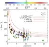 |
Fig. 17 Velocity profile for the O/B stars. The total velocity is plotted against the projected distance p to Sgr A*. Triangles denote fully known kinematics in three dimensions, squares denote only two-dimensional projected proper motion measurements and are therefore only lower limits of the total velocity. The colour-coding illustrates the normalised angular momentum |
The dashed lines show the escape velocity ve. Only one star has a velocity close to the escape velocity: Id 722. It is at a projected distance of 12.45′′ with vtot = (287 ± 27) km s-1. The proper motion of this star also points away from Sgr A*. For Fig. 17 we plot only the projected distances of the stars, which are only lower limits. The true distance of star Id 722 might well be larger. But when we consider the stellar mass distribution, the star’s velocity is lower than the escape velocity. The normalised angular momentum is h = 0.16, and if one takes the stellar mass into account for h as well, | h | becomes even smaller. This indicates that this star with ℳ = 32 ± 14 M⊙ is on a radial orbit, but the star is still gravitationally bound to the MW nuclear star cluster.
Some of the stars have large velocity uncertainties. Six stars may have velocities above the escape velocity (Id 366, 511, 610, 617, 728, and 853), four of them (610, 617, 728, 853) also have a low value of | h | < 0.2, suggesting either a high eccentricity or inclination in their orbits. To better constrain the stellar orbits, a more accurate radial velocity measurement is required.
5. Discussion
5.1. Detection of 19 new O/B stars
Our sample of 76 O/B stars mostly consists of previously known O/B stars. However, 24 O/B stars have not been reported before, and 19 of these O/B stars are probably also cluster member stars. Three stars (Id 663, 1104, and 3308) are possibly foreground stars, while two stars (Id 436, 3339) are definitely foreground stars.
To verify our classification as O/B type stars, we measured the equivalent widths of the CO line at 2.2935 μm and the Na I doublet at ~2.206 μm in Sect. 4.1 and compared the result to the mean value of the late-type stars. For most of the O/B stars, the equivalent widths deviate by ~3σ from the mean value of late-type stars for the CO line and by ~2σ from the mean late-type star value for Na I.
Only ten O/B stars have EWCO> 2.7 Å, i.e. within 3σ of the late-type stars’ mean value (EWCO,LT = 18.3). However, six of these ten stars have been classified as O/B stars in previous studies. For the other four stars (Id 718, 2446, 3308, and 3578), the significance of either the CO non-detection or of the Na non-detection is at least 2.7σ. The S/N of the spectra is in the range of 16.9 to 35.8, this is rather low compared to the O/B star median S/N of 46. It is possible that the low S/N or poorly subtracted light from surrounding late-type stars produces a weak CO line signal. If these stars indeed have weak CO lines, the low values of EWCO (3.2 Å−8.3 Å) would suggest effective temperatures Teff> 4500 K (Pfuhl et al. 2011). Then these stars could be of intermediate age (~100 Myr).
5.2. O/B star mass estimates
We estimated the masses of the O/B stars in Sect. 4.1.2 based on the assumptions that the intrinsic colours (H−KS)0 are in a narrow range, close to −0.10 (Straižys & Lazauskaitė 2009), their metallicity is roughly solar (Ramírez et al. 2000), and their ages are in the range of 3−8 Myr (Paumard et al. 2006; Lu et al. 2013). This means that we assumed the same age for the new O/B star detections as for the previously known O/B star population, for which this age estimate was derived. This may be an oversimplification. The new O/B-type stars are at larger projected distances from Sgr A* and may have formed in a different star formation event. This means that their age and metallicity may be different. Some of these stars have a mass of ~10 M⊙. Renzini et al. (1992) showed that a star with a mass ℳ = 9 M⊙ and solar metallicity spends ~20 Myr on the main sequence. This means that these stars may be much older than 3−8 Myr. On the other hand, among the new classified O/B stars are also several bright, massive stars (ℳ > 20 M⊙). These stars must be younger and close to the age of 3−8 Myr. The spectra of the newly identified O/B stars with S/N ≳ 50 contain a He I absorption line at 2.113 μm. Hanson et al. (1996) showed that this line disappears in early O stars. Therefore the stars with 2.113 μm absorption are later than O7 V, O7 III, or O9 I. This suggests that the new O/B stars belong to the same population as the already classified O/B stars, none of which is earlier than O7 (Paumard et al. 2006).
The estimated mass in Table B.2 is the median of the distribution of possible stellar masses weighted by the likelihood of the star position in the colour magnitude diagram. We considered the uncertainty of the Galactocentic distance σR0, the extinction law coefficient σα, the photometry (σH and σKS), and the intrinsic colour σ(H−KS)0 in the propagated uncertainty. For the brightest of these stars we derive median masses of more than 40 M⊙. Such a high mass was observed for O6 I or O6 V stars (Cox 2000, Table 15.8). But the stars with reported spectral type in our sample are of type O8 and later. For example, we derive a mass of  M⊙ for the O8−9.5 star Id 331. Stars of this spectral type have masses of ~28 M⊙ (O8 I star) and lower (Cox 2000, Table 15.8). This suggests that we rather overestimate the stellar masses.
We showed that the derived value for the extinction AKS from intrinsic colours is lower than the value of AKS from the extinction map adopted from Schödel et al. (2010; see Fig. 5). We would find better agreement by assuming an extinction law exponent of α = 2.1 instead of α = 2.21 (Schödel et al. 2010). Then the derived magnitudes KS,0 of the stars would be higher, that is, the stars would be fainter. We tested if this would lower the stellar masses, but found that it is only a minor effect. For most of the stars the lower limit of our mass estimate agrees with the mass expected for the spectral type.
5.3. Total mass of young stars
We calculated a lower limit for the total mass of young stars to  assuming a top-heavy initial mass function (IMF) with slope α = 1.7 (Lu et al. 2013) and a maximum stellar mass of 150 M⊙. This result agrees with the cluster total mass found by Lu et al. (2013) of 14 000 M⊙ to 37 000 M⊙ in the same integration range [M⊙;150 M⊙]. With an extremely top-heavy IMF (α = 0.45, Bartko et al. 2010), the mass is even higher
  , but still in agreement with Lu et al. (2013). We integrated up to stars with ℳ = 150M⊙, but the most massive star in the Galactic centre has only ℳ = 80M⊙ (Martins et al. 2007). When we integrate in the interval [1 M⊙;80 M⊙], the cluster mass is only
  , for α = 1.7, and
  for α = 0.45. We thus give ℳtotal,young ~ 12 000 M⊙ as a lower limit for the mass of the young star cluster.
For these calculations we assumed that the present-day mass function slope is the same as the IMF slope, but this is only valid for a simple stellar population (Elmegreen & Scalo 2006). This is a reasonable assumption, since we used stars in the mass range [30 M⊙;45 M⊙] to fit the IMF, and these stars should all be younger than 8 Myr. As we scaled the IMF only to the observed mass function of O/B stars and did not consider the massive and young emission-line stars, the derived total cluster mass is only a lower limit.
5.4. Disk membership
We estimated if an O/B star can be a member of the clockwise (CW) disk based on the stellar angular momentum h and on the stellar radial velocity vz. As the disk is receding in the SE and approaching in the NW, we can exclude the membership of stars with vz > 0 that are located in the NW and of stars with vz < 0 that are located in the SE. We can also exclude stars with an angular momentum h ≲ 0.5 if we can show that the orbit is not edge-on. This allowed us to exclude the CW disk membership for 53 stars (>69%) in our O/B star sample, of which 16 stars are newly classified O/B stars. When we assume that the CW disk is warped, as found by Bartko et al. (2009), these numbers change by only one star (54 stars, >72%).
A disk fraction of ≲30% agrees with the results of Yelda et al. (2014), who studied the kinematics of O/WR stars and found a disk fraction of ~20%. Yelda et al. (2014) also showed that the significance of the disk decreases with distance to Sgr A*. Our sample of new O/B stars mostly lies at ~10′′ (0.4 pc), that is, close to the assumed outer edge of the CW disk at ~13′′ (0.5 pc). It might be that the outer edge of the disk is even closer to Sgr A* (Støstad et al. 2015).
On the other hand, we found ten stars (one new) for which a membership to the CW disk is possible based on their proper motions, projected location, and radial velocity. However, this does not mean that these stars are necessarily members of the CW disk, as the three-dimensional location with respect to Sgr A* was not taken into account. We were unable to constrain whether the remaining 13 O/B stars might be members of the CW disk or not. The radial velocity uncertainty allows both a receding and an approaching motion, there is no proper motion available, or the inclination i is too high to determine the angular momentum h. Three of these undetermined stars are probably foreground stars.
For a better determination of the stellar orbits, a more sophisticated analysis such as that reported by Lu et al. (2009), Bartko et al. (2009), Yelda et al. (2014), and Sanchez-Bermudez et al. (2014), is necessary. In the future, the missing proper motions and radial velocities that are missing so far will probably also be available (Pfuhl et al., in prep.).
5.5. Origin of the early-type stars
Our data set covers the central 2.51 × 1.68 pc (>4 pc2) of the Galactic centre. No previous study covered such a large region with a comparable spatial resolution. We were able to extract stars as faint as KS = 15 mag with a completeness of 80% at KS ≈ 13.5 mag. For the bright supergiants and giant stars with KS < 13 mag, we can assume that our data set is roughly complete out to p = 0.84 pc (21′′).
Bright O/B stars with KS < 13 mag have a well-determined age of 3−8 Myr. We can add the red supergiant IRS 7, the emission-line stars, and sources with featureless spectra and KS < 13 mag, which are in the same age range. Then we find that 90% of these 79 massive stars are located within p = 0.44 pc (11.4′′). This confirms the finding of Støstad et al. (2015) that the cluster of young stars has an outer edge at ~13′′ (0.52 pc). This central confinement can help to constrain the origin and formation scenarios for the young stars.
It was suggested that young stars in the Galactic centre were formed in a massive young star cluster that fell towards the centre from r ≳10 pc (Gerhard 2001; McMillan & Portegies Zwart 2003). In this scenario the infalling cluster is stripped and disrupted. But then we would expect a higher number of young stars beyond p = 0.5 pc (Fujii et al. 2010; Perets & Gualandris 2010). Our data set contains only three bright early-type stars (and three faint early-type stars) beyond p = 0.5 pc, but 76 (23) within p = 0.5 pc. An infalling cluster would leave a trail of early-type stars, but we find no evidence for such a structure. It might be possible that the infalling cluster had been mass segregated and left a trail of fainter early-type stars that we could not detect. But other studies with a smaller spatial coverage but higher completeness for fainter stars were likewise unable to detect any signs of a trail (Bartko et al. 2010; Støstad et al. 2015).
The late-type stars are much less concentrated than the early-type stars. This agrees with the findings in other nuclear star clusters (e.g. Seth et al. 2010; Georgiev & Böker 2014; Carson et al. 2015). The old component of the nuclear star cluster is often spheroidal and more extended than the disk of young stars. One counterexample is NGC 4244, where the blue disk is more extended than the older spheroidal component (Seth et al. 2008b). Seth et al. (2006) argued that young stellar disks in nuclear star clusters have a lifetime of ≲1 Gyr before being disrupted. In other nuclear star clusters, the young disks are often aligned with the host galaxy disk (e.g. NGC 404, NGC 4244, and NGC 4449; Seth et al. 2006, 2008b; Georgiev & Böker 2014). This is not the case for the CW disk in the Galactic centre. The projected distribution of young stars beyond p = 0.47 pc (12′′) appears to be elongated along the Galactic plane, but slightly misaligned to it. It is unclear if this effect is only caused by the variable extinction.
The CW disk of young stars can be explained by in situ star formation in a dense disk or stream around Sgr A* (Levin & Beloborodov 2003; Paumard et al. 2006). The material would come from infalling molecular clumps and gas clouds (e.g. Wardle & Yusef-Zadeh 2008; Gualandris et al. 2012; Emsellem et al. 2015). As the stars are very concentrated in the centre, the star-forming region must have had a size of r ≲ 0.5 pc. However, the majority of the early-type stars in the Galactic centre are not on the CW disk (see Sect. 5.4 and Yelda et al. 2014). As the stars are only 3−8 Myr old, the young stars either did not all form in a disk or the disk is dissolving more rapidly than expected.
One possible disruption scenario is the infall of another molecular cloud to the Galactic centre (Mapelli et al. 2013). This cloud is disrupted in the supermassive black hole potential and forms an irregular, dense gas disk. Perturbations induced from this gas disk might be able to dismember the CW disk of young stars (Mapelli et al. 2013). This could explain the isotropic cluster of young stars in the same radial range as the CW disk. However, other reasons that cause an instability of the CW disk are also possible (e.g. Hobbs & Nayakshin 2009; Chen & Amaro-Seoane 2014). More simulations and theoretical work are needed to explore the possibilities.
5.6. Early-type stars beyond the central 0.5 pc
There are only six stars with projected distances p > 0.5 pc. These are three O/B stars (Id 982, 2048, and 2446) and three featureless sources (Id 161, 477, and 705). However, the classification of two of the O/B stars as cluster member stars is uncertain. Id 982 is located outside the coverage of the extinction map by Schödel et al. (2010), therefore the colour has a large uncertainty. Id 2048 lacks full colour information.
Id 2446 at p = 0.75 pc (19.5′′) is the only outer O/B star with available proper motions. The proper motion vector points away from Sgr A*, but the velocity is low enough for the star to be bound to the cluster (vpm = (43.5 ± 9.6) km s-1). The angular momentum is h = 0.01, which means that the star is on a radial projected orbit.
Two of the three featureless sources beyond 0.5 pc (Id 161/IRS 5 and 705/IRS 5NE) are part of the IRS 5 complex (Perger et al. 2008). Viehmann et al. (2006) pointed out that the IRS 5 sources are remarkably bright in the mid-infrared, but less prominent in the near-infrared. The O/B star Id 483/IRS 5SE also belongs to this group. IRS 5SE consists of two components, IRS 5SE1 and IRS 5SE2 (Viehmann et al. 2006), which cannot be resolved in our data set. In this region we have two additional spectra that we were unable to classify (IRS 5S and IRS 5E); the remaining stars in this area have late-type signatures.
Id 477/IRS 8 is a special case. This featureless source has the largest distance to Sgr A* of all early-type stars in our field of view. Geballe et al. (2006) classified IRS 8 as an O5−O6 giant or supergiant. This makes IRS 8 the earliest O/B star in the Galactic centre. All the O/B stars within p = 0.5 pc are of type O8 and later. This would make IRS 8 the youngest known star in the Galactic centre. However, Geballe et al. (2006) suggested that IRS 8 originally was a member of a close binary and was rejuvenated.
6. Summary
We observed the central >4 pc2 of the Galactic centre with the integral field spectrograph KMOS. Among more than 1000 spectra from single stars were 114 early-type star spectra. We analysed these early-type spectra, and found the following:
-
1.
We detected 24 previously unknown O/B-type stars. Of these,19 stars are probable cluster members. The newO/B stars are at projected distances of0.3 pc−0.92 pc and cover masses from ~10−40 M⊙.
-
2.
We derived a lower mass limit for the young cluster mass ℳtotal,young = 12 000 M⊙. We used different initial mass function slopes from the literature and integrated in the range ℳ = [1 M⊙;80 M⊙].
-
3.
With our spatially extended and nearly symmetric coverage, we studied the spatial distribution of early-type stars. We found that the early-type stars are strongly concentrated in the projected central p = 0.4 pc and that only a few stars lie beyond 0.5 pc. This contradicts a scenario where the early-type stars formed outside the Galactic centre in a massive cluster that fell towards the centre and depleted the stars at their current location. This formation scenario would leave behind a trail of early-type stars at projected distances of p > 0.5 pc, which we did not detect. This is a strong argument for the in situ formation of the early-type stars.
-
4.
We studied the kinematics of the O/B stars and showed that one of the new O/B stars is a good candidate to be a member of the clockwise rotating disk. However, the majority (≳69%) of the O/B stars is not on the disk. This means that either these stars have not formed on the clockwise disk or that the disk is already strongly disrupted. We found no stars that are unbound to the MW nuclear star cluster.
Online material
Appendix A: Spectral classification of emission-line stars
We have spectra of 29 emission line stars. These stars were classified in previous studies as either Ofpe/WN9 type, WN, or WC type stars. Ofpe/WN9 types have narrower lines and are cooler (Teff = 10 000−20 000 K) than WN and WC stars (Teff> 30 000 K). We found some disagreement with previously reported spectral classifications for some of the emission-line stars.
Id 144/AF and Id 1237/IRS 7E2(ESE): we find that the two stars Id 144/AF and Id 1237/IRS 7E2(ESE), which were listed as Ofpe/WN9 by Paumard et al. (2006), have broad emission lines and are rather WN8 or WN9 stars. Paumard et al. (2006) stated that their spectra of these stars are of high quality. But we also have a high S/N, 78.2 for Id 144/AF and 35.6 for Id 1237/IRS 7E2. Furthermore, the high-resolution spectra of Tanner et al. (2006) agree with Id 144/AF being a broad emission-line star, but they have no data for Id 1237/IRS 7E2(ESE). Paumard et al. (2003) also found a broad He I line in the spectrum of Id 144/AF. The resolving power R reported by Tanner et al. (2006) was 14 000 and 23 300, but only 1500 and 4000 in the data used by Paumard et al. (2006). Our data set with R = 4300 agrees with the high-resolution results from Tanner et al. (2006). Because of their broad emission lines (FWHM ~ 700 km s-1) and the resemblance of the spectra of Id 144/AF and Id 1237/IRS 7E2 with the WN8 and WN9 spectra in our data set, we classify Id 144/AF and Id 1237/IRS 7E2 as broad emission-line stars, probably WN8 or WN9. Id 1237/IRS 7E2 is also classified as a WN8 star by Martins et al. (2007). Martins et al. (2007) used non-LTE atmosphere models to derive the properties of Galactic centre stars. For Id 144/AF they found a degeneracy between the effective temperature Teff and the helium abundance He/H. In addition, the wind of this star could be stronger than the wind of the Ofpe/WN9 stars, and Id 144/AF may be more evolved. Martins et al. (2007) suggested that Ofpe/WN9 stars evolve to WN8 stars.
Id 666/IRS 7SW: we reclassify the star Id 666/IRS 7SW as WN8/WC9. This star was classified as WN8 in Paumard et al. (2006). The C III and C IV lines distinguish a WN8/WC9 star from a WN8 star. These lines are weaker than the He and H lines. Therefore a low S/N can lead to a misidentification as a WN8 star, but Paumard et al. (2006) state that their spectrum of Id. 666/IRS 7SW is of high quality. Our spectrum of this star has a S/N of 59.9, and we can clearly identify the C IV doublet at 2.0796 μm, and 2.0842 μm C III at 2.325 μm (see Fig. 11). The spectrum is very similar to the spectrum of the WN8/WC9 star Id 491/IRS 15SW, therefore we conclude that Id 666/IRS 7SW is also a WN8/WC9 type star. The two stars Id 491/IRS 15SW and Id 666/IRS 7SW are also in a similar location at the
colour-magnitude diagram ((H−KS)0 = −0.02 and −0.11, KS,0 = 9.40 and 9.59, Fig. 3), which confirms their similarity. This classification agrees with that of Martins et al. (2007).
Id 185/IRS 29N, Id 283/IRS 34, Id 303, and Id 638/IRS 29NE1: four of the eleven WC stars have only shallow emission lines in our data set. These stars are Id 185/IRS 29N, Id 283/IRS 34, Id 303, and Id 638/IRS 29NE1. The lines are very broad, but only weakly pronounced. Previous studies (Paumard et al. 2001; Tanner et al. 2006) did not detect any distinct He I emission for Id 185/IRS 29N, while Paumard et al. (2003) reported a broad He I emission line for the same star. Tanner et al. (2006) suggested that Id 638/IRS 29NE1 is variable and that the spectral features changed with time. Rafelski et al. (2007) studied the light curve of IRS 29N over a time line of ten years and found photometric variability. They suggested that these sources could be a wind-colliding binary system. Gamen et al. (2012) showed that stars can change their spectra within months.
Apart from the weak but broad lines, all the four sources are also very red ((H−KS)0> 0.55). Their continua rise steeply with wavelength. This is an indication that these sources are embedded in dust (see e.g. Geballe et al. 2006 for IRS 8). The continuum in the spectra might not be the stellar continuum, but the continuum of the circumstellar dust, which dominates the lines (Figer et al. 1999; Chiar & Tielens 2001). Therefore the emission lines appear only as weak, broad bumps in the spectrum.
Circumstellar dust is common for WC9 stars such as Id 185/IRS 29N and Id 283/IRS 34. For earlier types such as WC8, dust formation is rather uncommon and might indicate colliding winds (Sander et al. 2012). The two stars Id 303 and Id 638/IRS 29NE1 are WC8/9 stars. Id 303 is located close to the minispiral, at least in projection. So it might be a bow-shock that causes the reddening of Id 303. The bow-shock sources Id 161/IRS 5 and Id 25347/IRS 1W are probably also embedded WR stars (Tanner et al. 2005; Sanchez-Bermudez et al. 2014), but their emission lines are outshone by the bow-shock continuum. Id 638/IRS 29NE1, however, is not located inside the minispiral. But as mentioned earlier, the spectral features seem to change with time. This could be explained by circumstellar dust.
Id 243/IRS 34W: the star with a narrow emission line, Id 243/IRS 34W, has moderate reddening ((H−KS)0 = 0.24) and a steeply rising continuum. As Paumard et al. (2003) already pointed out, this star is fainter than the other stars with narrow emission lines (see also the colour–magnitude diagram, yellow circle with black cross, Fig. 3). The star Id 243/IRS 34W shows a long-term photometric variability (Ott et al. 1999; Paumard et al. 2003). Therefore this star may also be dust embedded. Id 243/IRS 34W is a LBV candidate, and Humphreys et al. (1999) showed for the case η Carinae that LBV eruptions are accompanied with circumstellar dust obscurations.
Appendix B: O/B star tables
O/B stars I.
O/B stars II.
O/B stars III.
We downloaded the extinction map from the CDS database. It turned out that the astrometry of the extinction map was wrong by a scale factor of 60. We reported this issue to CDS, and the astrometry was fixed on 26th March, 2015.
Acknowledgments
This research was supported by the DFG cluster of excellence Origin and Structure of the Universe (www.universe-cluster.de). C.J.W. acknowledges support through the Marie Curie Career Integration Grant 303912. This publication makes use of data products from the Two Micron All Sky Survey, which is a joint project of the University of Massachusetts and the Infrared Processing and Analysis Center/California Institute of Technology, funded by the National Aeronautics and Space Administration and the National Science Foundation. This research made use of the SIMBAD database (operated at CDS, Strasbourg, France). We would like to thank the ESO staff who helped us to prepare our observations and obtain the data. Special thanks go to Alex Agudo Berbel, Yves Jung, Ric Davis, and Lodovico Coccato for advice and assistance in the data reduction process. We are also grateful to Sebastian Kamann for providing us with his code PampelMuse. We thank Morgan Fouesneau, Iskren Georgiev, and Paco Najarro for discussions and suggestions. We finally thank the anonymous referee for comments and suggestions.
References
- Bartko, H., Martins, F., Fritz, T. K., et al. 2009, ApJ, 697, 1741 [NASA ADS] [CrossRef] [Google Scholar]
- Bartko, H., Martins, F., Trippe, S., et al. 2010, ApJ, 708, 834 [NASA ADS] [CrossRef] [Google Scholar]
- Becklin, E. E., & Neugebauer, G. 1968, ApJ, 151, 145 [NASA ADS] [CrossRef] [Google Scholar]
- Blum, R. D., Ramírez, S. V., Sellgren, K., & Olsen, K. 2003, ApJ, 597, 323 [NASA ADS] [CrossRef] [Google Scholar]
- Böker, T., Laine, S., van der Marel, R. P., et al. 2002, AJ, 123, 1389 [NASA ADS] [CrossRef] [Google Scholar]
- Bressan, A., Marigo, P., Girardi, L., et al. 2012, MNRAS, 427, 127 [NASA ADS] [CrossRef] [Google Scholar]
- Buchholz, R. M., Schödel, R., & Eckart, A. 2009, A&A, 499, 483 [NASA ADS] [CrossRef] [EDP Sciences] [Google Scholar]
- Cappellari, M., & Emsellem, E. 2004, PASP, 116, 138 [NASA ADS] [CrossRef] [Google Scholar]
- Carollo, C. M., Stiavelli, M., & Mack, J. 1998, AJ, 116, 68 [NASA ADS] [CrossRef] [Google Scholar]
- Carpenter, J. M. 2001, AJ, 121, 2851 [NASA ADS] [CrossRef] [Google Scholar]
- Carr, J. S., Sellgren, K., & Balachandran, S. C. 2000, ApJ, 530, 307 [NASA ADS] [CrossRef] [Google Scholar]
- Carson, D. J., Barth, A. J., Seth, A. C., et al. 2015, AJ, 149, 170 [NASA ADS] [CrossRef] [Google Scholar]
- Chatzopoulos, S., Fritz, T. K., Gerhard, O., et al. 2015, MNRAS, 447, 948 [NASA ADS] [CrossRef] [Google Scholar]
- Chen, X., & Amaro-Seoane, P. 2014, ApJ, 786, L14 [NASA ADS] [CrossRef] [Google Scholar]
- Chen, Y., Girardi, L., Bressan, A., et al. 2014, MNRAS, 444, 2525 [NASA ADS] [CrossRef] [Google Scholar]
- Chiar, J. E., & Tielens, A. G. G. M. 2001, ApJ, 550, L207 [NASA ADS] [CrossRef] [Google Scholar]
- Christopher, M. H., Scoville, N. Z., Stolovy, S. R., & Yun, M. S. 2005, ApJ, 622, 346 [NASA ADS] [CrossRef] [Google Scholar]
- Côté, P., Piatek, S., Ferrarese, L., et al. 2006, ApJS, 165, 57 [NASA ADS] [CrossRef] [MathSciNet] [Google Scholar]
- Cox, A. N., ed. 2000, Allen’s Astrophysical Quantities, 4th edn. [Google Scholar]
- Crowther, P. A., Lennon, D. J., Walborn, N. R., & Smartt. 2006, ArXiv e-prints [arXiv:astro-ph/0606717] [Google Scholar]
- Cunha, K., Sellgren, K., Smith, V. V., et al. 2007, ApJ, 669, 1011 [Google Scholar]
- Davies, R. I. 2007, MNRAS, 375, 1099 [NASA ADS] [CrossRef] [Google Scholar]
- Davies, R. I., Agudo Berbel, A., Wiezorrek, E., et al. 2013, A&A, 558, A56 [NASA ADS] [CrossRef] [EDP Sciences] [Google Scholar]
- den Brok, M., Peletier, R. F., Seth, A., et al. 2014, MNRAS, 445, 2385 [NASA ADS] [CrossRef] [Google Scholar]
- Do, T., Ghez, A. M., Morris, M. R., et al. 2009, ApJ, 703, 1323 [NASA ADS] [CrossRef] [Google Scholar]
- Do, T., Lu, J. R., Ghez, A. M., et al. 2013, ApJ, 764, 154 [NASA ADS] [CrossRef] [Google Scholar]
- Dong, H., Wang, Q. D., Cotera, A., et al. 2011, MNRAS, 417, 114 [NASA ADS] [CrossRef] [Google Scholar]
- Dutra, C. M., & Bica, E. 2001, A&A, 376, 434 [NASA ADS] [CrossRef] [EDP Sciences] [Google Scholar]
- Eckart, A., Genzel, R., Ott, T., & Schödel, R. 2002, MNRAS, 331, 917 [NASA ADS] [CrossRef] [Google Scholar]
- Eisenhauer, F., Genzel, R., Alexander, T., et al. 2005, ApJ, 628, 246 [NASA ADS] [CrossRef] [Google Scholar]
- Ekers, R. D., van Gorkom, J. H., Schwarz, U. J., & Goss, W. M. 1983, A&A, 122, 143 [NASA ADS] [Google Scholar]
- Elmegreen, B. G., & Scalo, J. 2006, ApJ, 636, 149 [NASA ADS] [CrossRef] [Google Scholar]
- Emsellem, E., Renaud, F., Bournaud, F., et al. 2015, MNRAS, 446, 2468 [NASA ADS] [CrossRef] [Google Scholar]
- Feldmeier, A., Neumayer, N., Seth, A., et al. 2014, A&A, 570, A2 [NASA ADS] [CrossRef] [EDP Sciences] [Google Scholar]
- Ferrarese, L., Côté, P., Dalla Bontà, E., et al. 2006, ApJ, 644, L21 [NASA ADS] [CrossRef] [Google Scholar]
- Figer, D. F., McLean, I. S., & Najarro, F. 1997, ApJ, 486, 420 [NASA ADS] [CrossRef] [Google Scholar]
- Figer, D. F., McLean, I. S., & Morris, M. 1999, ApJ, 514, 202 [NASA ADS] [CrossRef] [Google Scholar]
- Fritz, T. K., Gillessen, S., Dodds-Eden, K., et al. 2011, ApJ, 737, 73 [NASA ADS] [CrossRef] [Google Scholar]
- Fritz, T. K., Chatzopoulos, S., Gerhard, O., et al. 2014, ApJ submitted [arXiv:1406.7568] [Google Scholar]
- Frogel, J. A., Stephens, A., Ramírez, S., & DePoy, D. L. 2001, AJ, 122, 1896 [NASA ADS] [CrossRef] [Google Scholar]
- Fujii, M., Iwasawa, M., Funato, Y., & Makino, J. 2010, ApJ, 716, L80 [NASA ADS] [CrossRef] [Google Scholar]
- Gamen, R., Arias, J. I., Barbá, R. H., et al. 2012, A&A, 546, A92 [NASA ADS] [CrossRef] [EDP Sciences] [Google Scholar]
- Geballe, T. R., Najarro, F., Rigaut, F., & Roy, J.-R. 2006, ApJ, 652, 370 [NASA ADS] [CrossRef] [Google Scholar]
- Genzel, R., Schödel, R., Ott, T., et al. 2003, ApJ, 594, 812 [NASA ADS] [CrossRef] [PubMed] [Google Scholar]
- Georgiev, I. Y., & Böker, T. 2014, MNRAS, 441, 3570 [NASA ADS] [CrossRef] [Google Scholar]
- Gerhard, O. 2001, ApJ, 546, L39 [NASA ADS] [CrossRef] [Google Scholar]
- Ghez, A. M., Duchêne, G., Matthews, K., et al. 2003, ApJ, 586, L127 [NASA ADS] [CrossRef] [Google Scholar]
- Ghez, A. M., Salim, S., Hornstein, S. D., et al. 2005, ApJ, 620, 744 [NASA ADS] [CrossRef] [Google Scholar]
- Ghez, A. M., Salim, S., Weinberg, N. N., et al. 2008, ApJ, 689, 1044 [NASA ADS] [CrossRef] [Google Scholar]
- Gillessen, S., Eisenhauer, F., Fritz, T. K., et al. 2009a, ApJ, 707, L114 [NASA ADS] [CrossRef] [Google Scholar]
- Gillessen, S., Eisenhauer, F., Trippe, S., et al. 2009b, ApJ, 692, 1075 [NASA ADS] [CrossRef] [Google Scholar]
- Gosling, A. J., Bandyopadhyay, R. M., & Blundell, K. M. 2009, MNRAS, 394, 2247 [NASA ADS] [CrossRef] [Google Scholar]
- Graham, A. W., & Spitler, L. R. 2009, MNRAS, 397, 2148 [NASA ADS] [CrossRef] [Google Scholar]
- Gualandris, A., Mapelli, M., & Perets, H. B. 2012, MNRAS, 427, 1793 [NASA ADS] [CrossRef] [Google Scholar]
- Hanson, M. M., Conti, P. S., & Rieke, M. J. 1996, ApJS, 107, 281 [Google Scholar]
- Hanson, M. M., Kudritzki, R.-P., Kenworthy, M. A., Puls, J., & Tokunaga, A. T. 2005, ApJS, 161, 154 [NASA ADS] [CrossRef] [EDP Sciences] [MathSciNet] [Google Scholar]
- Herbst, T. M., Beckwith, S. V. W., Forrest, W. J., & Pipher, J. L. 1993, AJ, 105, 956 [NASA ADS] [CrossRef] [Google Scholar]
- Hobbs, A., & Nayakshin, S. 2009, MNRAS, 394, 191 [NASA ADS] [CrossRef] [Google Scholar]
- Horrobin, M., Eisenhauer, F., Tecza, M., et al. 2004, Astron. Nachr., 325, 88 [Google Scholar]
- Humphreys, R. M., Davidson, K., & Smith, N. 1999, PASP, 111, 1124 [NASA ADS] [CrossRef] [Google Scholar]
- Kamann, S., Wisotzki, L., & Roth, M. M. 2013, A&A, 549, A71 [NASA ADS] [CrossRef] [EDP Sciences] [Google Scholar]
- Krabbe, A., Genzel, R., Eckart, A., et al. 1995, ApJ, 447, L95 [NASA ADS] [CrossRef] [Google Scholar]
- Lau, R. M., Herter, T. L., Morris, M. R., Becklin, E. E., & Adams, J. D. 2013, ApJ, 775, 37 [NASA ADS] [CrossRef] [Google Scholar]
- Lauer, T. R., Bender, R., Kormendy, J., Rosenfield, P., & Green, R. F. 2012, ApJ, 745, 121 [NASA ADS] [CrossRef] [Google Scholar]
- Lee, S., Pak, S., Choi, M., et al. 2008, ApJ, 674, 247 [NASA ADS] [CrossRef] [Google Scholar]
- Levin, Y., & Beloborodov, A. M. 2003, ApJ, 590, L33 [NASA ADS] [CrossRef] [Google Scholar]
- Lu, J. R., Ghez, A. M., Hornstein, S. D., et al. 2009, ApJ, 690, 1463 [NASA ADS] [CrossRef] [Google Scholar]
- Lu, J. R., Do, T., Ghez, A. M., et al. 2013, ApJ, 764, 155 [NASA ADS] [CrossRef] [Google Scholar]
- Madigan, A.-M., Pfuhl, O., Levin, Y., et al. 2014, ApJ, 784, 23 [NASA ADS] [CrossRef] [Google Scholar]
- Mapelli, M., Gualandris, A., & Hayfield, T. 2013, MNRAS, 436, 3809 [NASA ADS] [CrossRef] [Google Scholar]
- Markwardt, C. B. 2009, in Astronomical Data Analysis Software and Systems XVIII, eds. D. A. Bohlender, D. Durand, & P. Dowler, ASP Conf. Ser., 411, 251 [Google Scholar]
- Martins, F., Schaerer, D., & Hillier, D. J. 2005, A&A, 436, 1049 [NASA ADS] [CrossRef] [EDP Sciences] [Google Scholar]
- Martins, F., Genzel, R., Hillier, D. J., et al. 2007, A&A, 468, 233 [NASA ADS] [CrossRef] [EDP Sciences] [Google Scholar]
- Martins, F., Hillier, D. J., Paumard, T., et al. 2008, A&A, 478, 219 [NASA ADS] [CrossRef] [EDP Sciences] [Google Scholar]
- McMillan, S. L. W., & Portegies Zwart, S. F. 2003, ApJ, 596, 314 [NASA ADS] [CrossRef] [Google Scholar]
- Morris, P. W., Eenens, P. R. J., Hanson, M. M., Conti, P. S., & Blum, R. D. 1996, ApJ, 470, 597 [NASA ADS] [CrossRef] [Google Scholar]
- Neumayer, N., Walcher, C. J., Andersen, D., et al. 2011, MNRAS, 413, 1875 [NASA ADS] [CrossRef] [Google Scholar]
- Nishiyama, S., & Schödel, R. 2013, A&A, 549, A57 [NASA ADS] [CrossRef] [EDP Sciences] [Google Scholar]
- Nishiyama, S., Nagata, T., Kusakabe, N., et al. 2006, ApJ, 638, 839 [NASA ADS] [CrossRef] [Google Scholar]
- Nishiyama, S., Tamura, M., Hatano, H., et al. 2009, ApJ, 696, 1407 [NASA ADS] [CrossRef] [Google Scholar]
- Ott, T., Eckart, A., & Genzel, R. 1999, ApJ, 523, 248 [NASA ADS] [CrossRef] [Google Scholar]
- Paumard, T., Maillard, J. P., Morris, M., & Rigaut, F. 2001, A&A, 366, 466 [NASA ADS] [CrossRef] [EDP Sciences] [Google Scholar]
- Paumard, T., Maillard, J.-P., & Stolovy, S. 2003, Astron. Nachr. Suppl., 324, 303 [NASA ADS] [CrossRef] [Google Scholar]
- Paumard, T., Maillard, J.-P., & Morris, M. 2004, A&A, 426, 81 [NASA ADS] [CrossRef] [EDP Sciences] [Google Scholar]
- Paumard, T., Genzel, R., Martins, F., et al. 2006, ApJ, 643, 1011 [NASA ADS] [CrossRef] [Google Scholar]
- Perets, H. B., & Gualandris, A. 2010, ApJ, 719, 220 [NASA ADS] [CrossRef] [Google Scholar]
- Perger, M., Moultaka, J., Eckart, A., et al. 2008, A&A, 478, 127 [NASA ADS] [CrossRef] [EDP Sciences] [Google Scholar]
- Pfuhl, O., Fritz, T. K., Zilka, M., et al. 2011, ApJ, 741, 108 [NASA ADS] [CrossRef] [Google Scholar]
- Pott, J.-U., Eckart, A., Glindemann, A., et al. 2005, The Messenger, 119, 43 [NASA ADS] [Google Scholar]
- Rafelski, M., Ghez, A. M., Hornstein, S. D., Lu, J. R., & Morris, M. 2007, ApJ, 659, 1241 [NASA ADS] [CrossRef] [Google Scholar]
- Ramírez, S. V., Sellgren, K., Carr, J. S., et al. 2000, ApJ, 537, 205 [NASA ADS] [CrossRef] [Google Scholar]
- Reid, M. J., & Brunthaler, A. 2004, ApJ, 616, 872 [NASA ADS] [CrossRef] [Google Scholar]
- Reijns, R. A., Seitzer, P., Arnold, R., et al. 2006, A&A, 445, 503 [NASA ADS] [CrossRef] [EDP Sciences] [Google Scholar]
- Renzini, A., Greggio, L., Ritossa, C., & Ferrario, L. 1992, ApJ, 400, 280 [NASA ADS] [CrossRef] [Google Scholar]
- Rossa, J., van der Marel, R. P., Böker, T., et al. 2006, AJ, 132, 1074 [NASA ADS] [CrossRef] [Google Scholar]
- Sabha, N., Witzel, G., Eckart, A., et al. 2010, A&A, 512, A2 [NASA ADS] [CrossRef] [EDP Sciences] [Google Scholar]
- Sanchez-Bermudez, J., Schödel, R., Alberdi, A., et al. 2014, A&A, 567, A21 [NASA ADS] [CrossRef] [EDP Sciences] [Google Scholar]
- Sander, A., Hamann, W.-R., & Todt, H. 2012, A&A, 540, A144 [NASA ADS] [CrossRef] [EDP Sciences] [Google Scholar]
- Schödel, R., Eckart, A., Alexander, T., et al. 2007, A&A, 469, 125 [NASA ADS] [CrossRef] [EDP Sciences] [Google Scholar]
- Schödel, R., Merritt, D., & Eckart, A. 2009, A&A, 502, 91 [NASA ADS] [CrossRef] [EDP Sciences] [Google Scholar]
- Schödel, R., Najarro, F., Muzic, K., & Eckart, A. 2010, A&A, 511, A18 [NASA ADS] [CrossRef] [EDP Sciences] [Google Scholar]
- Schödel, R., Feldmeier, A., Kunneriath, D., et al. 2014a, A&A, 566, A47 [NASA ADS] [CrossRef] [EDP Sciences] [Google Scholar]
- Schödel, R., Feldmeier, A., Neumayer, N., Meyer, L., & Yelda, S. 2014b, Class. Quant. Grav., 31, 244007 [NASA ADS] [CrossRef] [Google Scholar]
- Scott, N., & Graham, A. W. 2013, ApJ, 763, 76 [NASA ADS] [CrossRef] [Google Scholar]
- Scoville, N. Z., Stolovy, S. R., Rieke, M., Christopher, M., & Yusef-Zadeh, F. 2003, ApJ, 594, 294 [Google Scholar]
- Seth, A. C., Dalcanton, J. J., Hodge, P. W., & Debattista, V. P. 2006, AJ, 132, 2539 [NASA ADS] [CrossRef] [Google Scholar]
- Seth, A., Agüeros, M., Lee, D., & Basu-Zych, A. 2008a, ApJ, 678, 116 [NASA ADS] [CrossRef] [Google Scholar]
- Seth, A. C., Blum, R. D., Bastian, N., Caldwell, N., & Debattista, V. P. 2008b, ApJ, 687, 997 [NASA ADS] [CrossRef] [Google Scholar]
- Seth, A. C., Cappellari, M., Neumayer, N., et al. 2010, ApJ, 714, 713 [NASA ADS] [CrossRef] [Google Scholar]
- Sharples, R., Bender, R., Agudo Berbel, A., et al. 2013, The Messenger, 151, 21 [NASA ADS] [Google Scholar]
- Skrutskie, M. F., Cutri, R. M., Stiening, R., et al. 2006, AJ, 131, 1163 [NASA ADS] [CrossRef] [Google Scholar]
- Smith, I. L., & Wardle, M. 2014, MNRAS, 437, 3159 [NASA ADS] [CrossRef] [Google Scholar]
- Stead, J. J., & Hoare, M. G. 2009, MNRAS, 400, 731 [NASA ADS] [CrossRef] [Google Scholar]
- Støstad, M., Do, T., Murray, N., et al. 2015, ApJ, 808, 106 [NASA ADS] [CrossRef] [Google Scholar]
- Straižys, V., & Lazauskaitė, R. 2009, Balt. Astron., 18, 19 [NASA ADS] [Google Scholar]
- Tang, J., Bressan, A., Rosenfield, P., et al. 2014, MNRAS, 445, 4287 [NASA ADS] [CrossRef] [Google Scholar]
- Tanner, A., Ghez, A. M., Morris, M. R., & Christou, J. C. 2005, ApJ, 624, 742 [NASA ADS] [CrossRef] [Google Scholar]
- Tanner, A., Figer, D. F., Najarro, F., et al. 2006, ApJ, 641, 891 [NASA ADS] [CrossRef] [Google Scholar]
- van Dokkum, P. G. 2001, PASP, 113, 1420 [NASA ADS] [CrossRef] [Google Scholar]
- Viehmann, T., Eckart, A., Schödel, R., Pott, J.-U., & Moultaka, J. 2006, ApJ, 642, 861 [NASA ADS] [CrossRef] [Google Scholar]
- Walcher, C. J., Böker, T., Charlot, S., et al. 2006, ApJ, 649, 692 [NASA ADS] [CrossRef] [Google Scholar]
- Wallace, L., & Hinkle, K. 1996, ApJS, 107, 312 [NASA ADS] [CrossRef] [Google Scholar]
- Wang, Q. D., Dong, H., Cotera, A., et al. 2010, MNRAS, 402, 895 [NASA ADS] [CrossRef] [Google Scholar]
- Wardle, M., & Yusef-Zadeh, F. 2008, ApJ, 683, L37 [NASA ADS] [CrossRef] [Google Scholar]
- Wehner, E. H., & Harris, W. E. 2006, ApJ, 644, L17 [NASA ADS] [CrossRef] [Google Scholar]
- Yelda, S., Ghez, A. M., Lu, J. R., et al. 2014, ApJ, 783, 131 [NASA ADS] [CrossRef] [Google Scholar]
- Yusef-Zadeh, F., Stolovy, S. R., Burton, M., Wardle, M., & Ashley, M. C. B. 2001, ApJ, 560, 749 [NASA ADS] [CrossRef] [Google Scholar]
- Zhao, J.-H., Morris, M. R., Goss, W. M., & An, T. 2009, ApJ, 699, 186 [NASA ADS] [CrossRef] [Google Scholar]
All Tables
All Figures
|
Fig. 1 Field of view and spatial distribution of early-type stars in the MW nuclear star cluster. The black box shows the KMOS 64.̋9 × 43.̋3 field of view, i.e. 2.51 × 1.68 pc, the small square in the upper middle was not observed due to the inactive IFU 13. Blue lines are the equatorial coordinate grid with a spacing of 10′′. The dashed blue horizontal line denotes the orientation of the Galactic plane. The black cross shows the position of Sgr A*. The underlying image is from HST/NICMOS (Dong et al. 2011), aligned along Galactic coordinates. Yellow diamond symbols denote confirmed Wolf-Rayet (WR) and emission-line stars, cyan squares are stars with featureless spectra, green circles denote O/B stars. Red ×-symbols indicate new young star candidates, blue plus-symbols probable foreground stars. The red line denotes the line of nodes of the clockwise-rotating disk of young stars. |
| In the text | |
|
Fig. 2 Number density profile of the spectroscopic data set in different magnitude bins. |
| In the text | |
|
Fig. 3 Colour–magnitude diagram of the stars within the KMOS field of view with extracted spectra and H and KS photometry, after extinction correction. Stars with colours −0.5 mag are most likely foreground stars (left of the vertical line). Different symbols and colours denote different types of stars. Yellow circles denote emission-line/WR stars, cyan squares are sources with featureless spectra, green triangles are O/B type stars, grey dots are late-type stars, black plus-signs are stars of uncertain type. The right y-axis denotes the KS magnitude after extinction correction, with a mean extinction of AKS = 2.70 mag. |
| In the text | |
|
Fig. 4 Spectra of the newly identified O/B type stars. The fluxes are normalised and an offset is added to the flux. The spectra are not shifted to rest wavelength. The numbers denote the identification numbers of the stars as listed in Tables B.1−B.3. We also show the S/N and denote probable foreground stars with “fg”. |
| In the text | |
|
Fig. 5 Comparison of the extinction AKS in magnitudes derived from the intrinsic colour with the extinction from the extinction map of Schödel et al. (2010) for O/B stars. The black line denotes the 1:1 line, blue squares are foreground stars, red triangles are cluster member stars. Typical error bars are shown in the lower right corner. |
| In the text | |
|
Fig. 6 Cumulative mass distribution of star Id 617. The horizontal lines denote 0.16, 0.5, and 0.86 percentiles, the vertical lines denote the corresponding masses. We derived a mass of |
| In the text | |
|
Fig. 7 Emission line map of Br γ gas at 2.1661 μm of the full KMOS mosaic. The axes show the distance from Sgr A* (red plus sign) in Galactic coordinates. Black crosses with cyan surrounding square symbols denote the positions of the sources with featureless spectra (see Sect. 4.3). The flux of Br γ emission is not saturated, but the scaling was set low in order to show the fainter, extended structure of the minispiral. |
| In the text | |
|
Fig. 8 Same as Fig. 7 for He I gas at 2.0587 μm. The black plus sign denotes the position of Sgr A*. The He I emission line is weaker than the Br γ line. Black crosses with yellow surrounding square symbols denote the positions of the emission-line stars (see Sect. 4.2.3). The He I line flux is not saturated in the data, but we set the scaling in this image low in order to show the extended structure of the minispiral. |
| In the text | |
|
Fig. 9 Same as Fig. 7 for H2 gas at 2.1218 μm. The red plus sign denotes the position of Sgr A*. The H2 line flux is not saturated in the data, but we set the scaling in this image low in order to show the extended structure of the gas. |
| In the text | |
|
Fig. 10 Spectra of stars with narrow emission lines and Wolf-Rayet stars. The lower six spectra are Ofpe/WN9 stars with narrow emission lines (FWHM ~ 200 km s-1). Fluxes are normalised and an offset is added to the flux. The spectra are not shifted to rest wavelength. The narrow emission line in the 2.167 μm emission line of spectrum Id 1237 is a residual of poorly subtracted minispiral emission. |
| In the text | |
|
Fig. 11 Spectra of Wolf-Rayet stars of type WN and WN/WC, ordered by increasing WN-type from bottom to top. The fluxes are normalised and an offset is added to the flux. The spectra are not shifted to rest wavelength. |
| In the text | |
|
Fig. 12 Spectra of Wolf-Rayet stars of type WC. The classification from Paumard et al. (2006, PGM2006) is written for all spectra. The narrow emission line at 2.167 μm of spectrum Id 784 is a residual of the subtracted minispiral emission. The fluxes are normalised and an offset is added to the flux. The spectra are not shifted to rest wavelength. |
| In the text | |
|
Fig. 13 Featureless spectra. Emission lines are due to imperfect background subtraction and caused by He I, H I, and H2 gas emission. The fluxes are normalised and an offset is added to the flux. The spectra are not shifted to rest wavelength. |
| In the text | |
|
Fig. 14 Cumulative number counts of early-type stars (blue plus signs) and late-type stars (red crosses) as a function of projected distance p from Sgr A*, normalised to one. Foreground stars were excluded. |
| In the text | |
|
Fig. 15 Stellar surface density profile for all early-type stars (O/B, emission line stars, and sources with featureless spectra). We exclude possible foreground stars and apply a completeness correction (see Sect. 3.1). We consider only stars brighter than KS = 14.3. Black triangles denote this study, red squares the results of Do et al. (2013). |
| In the text | |
|
Fig. 16 Three-dimensional stellar kinematics of the O/B stars and emission line stars (smaller arrows). The arrows denote the proper motions, colours signify different radial velocities vz. The black cross indicates the position of Sgr A*. The coordinates show the offset to Sgr A* in equatorial coordinates, the numbers at the top and left denote absolute equatorial coordinates. The Galactic plane is plotted as a blue dashed line, and the line of nodes of the clockwise disk with Ω = 96° is shown as a red line. The green dot-dashed line illustrates the projected rotation axis of the clockwise disk. |
| In the text | |
|
Fig. 17 Velocity profile for the O/B stars. The total velocity is plotted against the projected distance p to Sgr A*. Triangles denote fully known kinematics in three dimensions, squares denote only two-dimensional projected proper motion measurements and are therefore only lower limits of the total velocity. The colour-coding illustrates the normalised angular momentum |
| In the text | |
Current usage metrics show cumulative count of Article Views (full-text article views including HTML views, PDF and ePub downloads, according to the available data) and Abstracts Views on Vision4Press platform.
Data correspond to usage on the plateform after 2015. The current usage metrics is available 48-96 hours after online publication and is updated daily on week days.
Initial download of the metrics may take a while.