| Issue |
A&A
Volume 570, October 2014
|
|
|---|---|---|
| Article Number | A93 | |
| Number of page(s) | 9 | |
| Section | The Sun | |
| DOI | https://doi.org/10.1051/0004-6361/201424377 | |
| Published online | 23 October 2014 | |
Conversion from mutual helicity to self-helicity observed with IRIS⋆
1
Key Laboratory of Solar Activity, National Astronomical Observatories,
Chinese Academy of Sciences,
100012
Beijing,
PR China
e-mail:
lepingli@nao.cas.cn
2
Max-Planck Institute for Solar System Research
(MPS), 37077
Göttingen,
Germany
Received: 11 June 2014
Accepted: 8 September 2014
Context. In the upper atmosphere of the Sun observations show convincing evidence for crossing and twisted structures, which are interpreted as mutual helicity and self-helicity.
Aims. We use observations with the new Interface Region Imaging Spectrograph (IRIS) to show the conversion of mutual helicity into self-helicity in coronal structures on the Sun.
Methods. Using far UV spectra and slit-jaw images from IRIS and coronal images and magnetograms from SDO, we investigated the evolution of two crossing loops in an active region, in particular, the properties of the Si IV line profile in cool loops.
Results. In the early stage two cool loops cross each other and accordingly have mutual helicity. The Doppler shifts in the loops indicate that they wind around each other. As a consequence, near the crossing point of the loops (interchange) reconnection sets in, which heats the plasma. This is consistent with the observed increase of the line width and of the appearance of the loops at higher temperatures. After this interaction, the two new loops run in parallel, and in one of them shows a clear spectral tilt of the Si IV line profile. This is indicative of a helical (twisting) motion, which is the same as to say that the loop has self-helicity.
Conclusions. The high spatial and spectral resolution of IRIS allowed us to see the conversion of mutual helicity to self-helicity in the (interchange) reconnection of two loops. This is observational evidence for earlier theoretical speculations.
Key words: Sun: transition region / Sun: UV radiation / Sun: chromosphere / techniques: spectroscopic / line: profiles
Movie associated with Fig. 1 and Appendix A are available in electronic form at http://www.aanda.org
© ESO, 2014
1. Introduction
Magnetic helicity is a key quantity that characterizes the complexity of a magnetic configuration in terms of topology and of the linkage of magnetic field lines. When a magnetic structure is built up by two (or more) substructures, one can introduce the concept of self-helicity and mutual helicity (Berger 1999). Self-helicity corresponds to the twist and writhe of confined bundles of magnetic flux, while mutual helicity characterizes the crossing of field lines in the magnetic configuration (Régnier et al. 2005). Using TRACE images, Chae (2000) determined the mutual helicity of filaments based on two crossing threads. For the active region (AR) NOAA 8210, Régnier et al. (2005) reported that the magnetic configuration was dominated by mutual helicity and not by self-helicity. With theoretical arguments, Berger (1999) speculated that mutual helicity can be converted into self-helicity if two magnetic loops reconnect. Georgoulis (2011) proposed that numerous small-scale magnetic reconnection events can lead to an effective transformation of mutual into self-magnetic helicity. Tziotziou et al. (2013) found a hysteresis in the buildup of self-helicity with respect to mutual helicity, and considered this as a possible conversion of mutual- into self-helicity. They also suggested that magnetic reconnection is the way to achieve this. However, as of today, there is no observational confirmation for the conversion from mutual into self-helicity or vice versa.
General information of IRIS raster scans and slit-jaw images.
One way to detect self-helicity is to investigate the spectral tilt of an emission line. In the image of a spectral line in a slit spectrometer (i.e., space vs. wavelength), a static bright feature appears as a line along the wavelength direction that is perpendicular to the slit direction. However, if the structure shows a spinning motion, one side of the feature will show a redshift, the other a blueshift. This leads to a tilt of the line, so that the bright feature in the spectral image is no longer perpendicular to the slit direction. In spectral images this is easy to see and is often called spectral tilt. The detection of this spinning motion is similar to the detection of a spectroscopic binary.
The spinning nature of spicular features was found by investigating the spectral tilt in Hα spectra (Pasachoff et al. 1968; Rompolt 1975). Cook et al. (1984) observed the spectral tilt in transition region emission features in C IV spectra. Pike & Mason (1998) reported blueshift and redshift on opposite sides of macrospicules and interpreted them as a rotating motion. Tian et al. (2008) reported both red and blue Doppler shifts in bright points and proposed that this might result from a twist of the associated magnetic loop system. Kamio et al. (2010) detected redshift and blueshift on two sides of a macrospicule and explained this with the unfolding motion of a twisted magnetic flux rope. Curdt & Tian (2011) reported simultaneous Doppler flows of a red and a blue component without apparent motion and considered this as spectroscopic evidence for helicity in explosive events. Based on observations of bifurcated structures and spectral tilt, Curdt et al. (2012) proposed that there are spinning motions in transition region jets. De Pontieu et al. (2012) detected a spectral line tilt in off-limb spicules, which they considered to be the signature of torsional motion. Orozco Suárez et al. (2012) found opposite Doppler shifts at the edge of a prominence foot and interpreted these shifts as prominence plasma that rotates around the axis. Recently, Wedemeyer et al. (2013) and Su et al. (2014) separately found redshifted and blueshifted regions on the two sides of the prominence leg and proposed that there is rotational motion in a tornado-like prominence.
All these observations together show that spinning and twisting motions are common on the Sun. New observations with the Interface Region Imaging Spectrograph (IRIS; De Pontieu et al. 2014a) now clearly show that these torsional motions related to self-helicity are a ubiquitous feature of the solar atmosphere (De Pontieu et al. 2014b). With the common observations of mutual helicity, that is, crossing of loops, threads, and so on, the question arises whether these two forms of helicity are converted into each other, as speculated by Berger (1999).
To determine whether there is a helicity conversion, we mainly employed spectra and images of the transition region acquired by IRIS. Adding context data of the corona and the photospheric magnetic field, we investigated the change of the mutual and self-helicity of two cool loops in an active region. Our results clearly indicate that mutual helicity is converted into self-helicity.
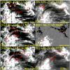 |
Fig. 1 IRIS slit-jaw images and context from AIA and HMI. The left panels a)−c) show snapshots of the IRIS slit-jaw images during the three raster scans. The right panels show the SDO context: the AIA 304 Å image d) and the HMI LOS magnetogram e) during the first scan, and the AIA 171 Å image f) during the third scan. The yellow dotted lines in panels a) and d) outline the envelope containing the two cool loops seen in the IRIS slit-jaw images. The red circles mark the endpoints of these loops. The green arrows in a) and b) indicate the crossing point. The red dashed lines in b) and c) show the positions for time-space diagrams displayed in Fig. 3. The green rectangles in b) and c) are the FOV of Figs. 4 and 6. The center of this image is at solar (x,y) = (319″,102″), and the FOV is 75″ × 50″. The temporal evolution of the IRIS slit-jaw images at 1400 Å of the AIA 304 Å and 171 Å channels the HMI magnetograms is available in the online edition. |
2. Observations and data processing
The IRIS observatory provides simultaneous images and spectra of the photosphere, chromosphere, transition region, and corona (De Pontieu et al. 2014a). From 05:00 UT to 08:00 UT on September 27, 2013, IRIS observed the active region AR 11850 and acquired three raster scans with the slit spectrograph. The two loops we concentrate on here are located to the north of the AR. As we show below, the first and second observing sequences were made during a phase of mutual helicity, the third raster during a self-helicity phase. We used IRIS level 2 data, which are already corrected for flatfield, geometric distortions, and dark current1. The general information on the observations is listed in Table 1. For the first and second scans, large dense raster modes are employed with steps of 0.35′′. For the third scan, a coarse raster mode with steps of 2′′ is used. During the first two scans, all available wavelength bands are included in the slit-jaw images (SJI), that is, 1330 Å, 1400 Å, 2796 Å, and 2832 Å. In the third scan, only images in the 1400 Å band are recorded. We scaled the maps and images to the same pixel scale for all scans and co-aligned all IRIS data according to the information in Table 1. Figures 1a−c separately show the IRIS 1400 Å band SJI images during the three observing sequences.
To place the IRIS data in the context of the structure and evolution from the photosphere to the corona we used data from the Solar Dynamics Observatory (SDO; Pesnell et al. 2012), in particular, of the Atmospheric Imaging Assembly (AIA; Lemen et al. 2012) and the Helioseismic and Magnetic Imager (HMI; Schou et al. 2012). The time cadence and spatial sampling of the AIA images are 12 s and 0.6′′/pixel. For the HMI line-of-sight (LOS) magnetograms the respective numbers are 45 s and 0.5′′/pixel. We scaled the SDO observations to match the IRIS SJI and co-aligned them using several characteristic features, such as network and plage patterns. Figures 1d−f show an AIA 304 Å image, an HMI magnetogram, and an AIA 171 Å image taken during the IRIS observations. A movie showing the temporal evolution of the Sun as seen in the IRIS and SDO data is available online.
IRIS scans the whole structure for the second and third raster scans. During the first raster scan the IRIS spectral data only cover the left half of the field of view (FOV) shown in Fig. 1, however. Therefore, we mainly used the spectra of the second and third raster scans to investigate the properties of these two loops. For the spectroscopic analysis we used the transition region lines of Si IV at 1394 Å and 1403 Å. For the first two scans we used the 1394 Å line because it is stronger. During the third raster scan only the 1403 Å line has been recorded. The Si IV profiles were approximated by single-Gaussian fits with a continuum to build maps of intensity, Doppler shift, and line width.
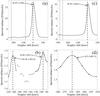 |
Fig. 2 Line profiles used for wavelength calibration averaged over the whole FOV of the raster map. Panels a) and b) show the profile during the second raster. The main target line Si IV at 1394 Å is visible in a). The vertical dotted lines indicate the wavelength region shown in panel b), where we zoom in on the lines of Ni II and Fe II that were used for wavelength calibration. The pluses show the actual observed spectrum, the solid line a spline fit around the center of the calibration lines. The vertical dashed lines indicate the peak of the spline fit. Panels c) and d) show the same for the third raster scan in the self-helicity phase. Here the S I line was used for wavelength calibration and the main target line was Si IV at 1403 Å. The count rate is per 0.166′′×0.166′′ pixel. |
For the Doppler maps a wavelength calibration is required, and we used the average spectra of the full FOV of each raster scan for this. Figure 2 shows the average spectra for the region around the 1394 Å (a, b) and 1403 Å (c, d) lines in the second and third raster scans. The lower panels show the (weaker) calibration lines alone. In the first and second scans these are the Ni II and Fe II lines, in the third scan this is the S I line (see Table 2 for a list of these lines). In part because of shortness of the scans, which lasted for half an hour or less, we verified that we did not have to correct the Doppler shifts for the orbital motion of the spacecraft.
3. Mutual helicity of two loops
During the first and the second raster scans, two cool loops crossing each other are visible in the IRIS 1400 Å SJI (Figs. 1a, b). The crossing point is marked by green arrows in Figs. 1a and b. These loops show emission from the Si IV lines and not the continuum that also contributes to the SJI. This is clearly evident from comparing these SJI with the spectroheliograms in Si IV that were derived from the spectral profiles of Si IV. These loops show plasma at temperatures of about 105 K. They connect two plage-type faculae of the active region with opposite polarities (cf. the magnetogram in Fig. 1e) and have lengths of about 40 Mm.
According to earlier work (Berger 1999; Régnier et al. 2005), these two loops should have mutual helicity because they cross each other. Therefore, we call the time span covered by the first two scans with the crossing loops the mutual-helicity phase below.
To better compare the AIA 304 Å images we also overplot the envelope of the two loops as derived from the IRIS 1400 Å image (Fig. 1a) on top of the AIA image (Fig. 1d, yellow dotted lines). In principle, the He II line dominating the AIA 304 Å channel and the Si IV lines form at similar temperatures just below 105 K. However, the AIA 304 Å channel is also very sensitive to cool material that is absorbed in the Ly-continua of H I and He I. This is contrast to the 1400 Å emission in IRIS images because this is longward of the Ly edge at 911 Å. This is the reason why the AIA 304 Å image looks quite different from the IRIS 1400 Å channel: while the latter shows the cool loop, in the AIA 304 Å channel a dark mini-filamentary structure is visible that highlights the cool material caught on fieldlines next to the Si IV loops. At least in the early phase of the first raster scan, there is no signature in the 171 Å channel of AIA, which underlines that the loops seen in IRIS are indeed cool loops. Later the 171 Å channel shows loops alongside the cool IRIS loops, which indicates heating of the loop system (see movie attached to Fig. 1).
In this mutual-helicity phase (during the first two raster scans), apparent motions along the loops can be seen in the movies of the IRIS 1400 Å SJI. Like leaves in the wind, bright blobs stream along the loops. In Figs. 3a and b we show time-space plots of IRIS 1400 Å SJI during the second raster scan (along lines AB and CD in Fig. 1b). We see several blobs moving toward the footpoints of the loops (at B and D) with apparent motions ranging from 30 km s-1 to 65 km s-1.
3.1. Motion and interaction of two loops
To investigate the motion of the two loops we studied the parameters of the (single-) Gaussians fitted to the line profile of Si IV. They are shown in Fig. 4 for the second raster scan, that is, in the mutual-helicity phase. The intensity map shows the same cool loops as the slit-jaw image (Fig. 1b). The loop crossing occurs near the line marked f.
The Doppler map in Fig. 4b reveals the general motion of the two loops. Left of the crossing point, loop 1 shows a redshift and loop 2 a blueshift. On the right side, loop 2 now shows a redshift and loop 1 a slight blueshift. For a better view, we display the spectra of Si IV at 1394 Å in Fig. 5 along the spatial locations indicated by the vertical dashed lines a−i in Fig. 4. The red markers in Fig. 5 denote the positions of loop 1, the green markers the positions of loop 2. At all these cuts, except for the cut at the crossing point, f, the two loops can be clearly distinguished in the spectra. This more detailed look at the spectra (which are not strictly single-Gaussian as assumed for the fits) confirms the above description of the (line-of-sight) motion of the loops.
Most importantly, there are several faint randomly distributed short-lived signatures of internal helical motions for both loops (spectral tilts in Figs. 5c, d, and h for loop 1, and Figs. 5a, b, and h for loop 2). The only long-lived signature for a spectral tilt is found at the crossing of the loop (cut f, Fig. 5f). This is also the only place where the Si IV line becomes very broad, which is very clear from the line width plot in Fig. 4c. At other locations along the loop, the line width is typically only some 15 km s-1 to 20 km s-1, while near the crossing point it is twice as broad (cf. the arrow in Fig. 4c). Therefore the spectral tilt at location f might be more an indication of the (small-scale) activity due to the interaction of the two loops than of a helical motion.
We also checked the profiles of the Mg II k line at 2796 Å that originates from chromospheric plasma. Figures A.1 and A.2 show the two loops during the second scan in the mutual-helicity phase. Even though the signal from Mg II is much fainter, we obtain similar results as for the Si IV line (see more details in Appendix A).
3.2. Scenario for loop interaction
The Doppler motions of the loops in the mutual-helicity phase indicate that the two loops wind around each other, interlocked near the crossing point. At the crossing point the magnetic fields hosting the two loops interact, which could lead to reconnection at that place. On the one hand, this would explain the increased line width seen at the crossing point, which would be a signature of the heating process that accompanies reconnection. On the other hand, the reconnection would accelerate material along the field lines, hence the loops, away from the crossing points in the direction of the footpoints, which would be consistent with the apparent motion seen in the slit-jaw images discussed above. Another consequence of that heating process are loops in the 171 Å channel of AIA in the later mutual-helicity phase (see movie attached to Fig. 1). These indicate hotter plasma that is found in loops next to the cool loops of the IRIS slit-jaw images.
In brief, these observations are consistent with a scenario in which the two loops have mutual helicity and wind around each other, followed by reconnection at the crossing point.
4. Conversion to self-helicity
Lines of interest.
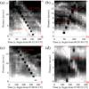 |
Fig. 3 Proper motions along the Si IV loops. Time-space plots of a series of IRIS slit-jaw images at 1400 Å along the dashed lines AB a), CD b), EF c), and GH d), as marked in Figs. 1b and c. The red dashed lines show motions along the loops. The respective velocities are denoted by the numbers in the plots. |
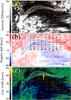 |
Fig. 4 Maps of intensity a), Doppler shift b), and line width c) of Si IV (1394 Å) for the second raster scan in the mutual-helicity phase. The dotted lines highlight the location of the two cool loops. The dashed lines a−i in a) and b) indicate the positions of the spectra shown in Fig. 5. The yellow arrow in c) marks a region with enhanced line width. The location of the maps is indicated in Fig. 1b. The FOV is 60.5″ × 33.3″. |
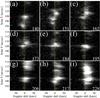 |
Fig. 5 Line profiles of Si IV (1394 Å) during the mutual-helicity phase. The spatial location of these spectra is indicated in Fig. 4 by the vertical dashed lines a−i. The red and green markers show the location of the two loops (red and green dotted lines in Fig. 4a). The numbers in the plot indicate the raster index, the vertical dotted lines the zero Doppler shift. |
4.1. Loops after interaction
After the interaction of the two loops, the situation changes quite dramatically, as can be seen in Fig. 1c, which displays an IRIS 1400 Å SJI during the third raster scan. As we show below, this phase shows signatures of self-helicity, which is why we call this the self-helicity phase.
After the interaction, one of the two loops remains visible in full length (labeled loop 1 in the figures). However, the middle part of the other loop disappears (loop 2). By combining the simultaneous AIA/SDO 171 Å images, we found that these two Si IV loops basically run parallel after the interaction. In particular, the Si IV loops are now also visible in the 171 Å channel of AIA (Fig. 1f), which is different from the earlier mutual-helicity phase. The 171 Å channel mainly shows plasma just below 106 K. That the loops in the AIA 171 Å images are roughly co-spatial with the cool Si IV loops indicates that (part of) the plasma is heated in response to the reconnection process2. The temporal evolution of the AIA 171 Å emission is shown in the movie attached to Fig. 1.
Similar to the mutual-helicity phase, bright blobs also move along the loops during the self-helicity phase. Figures 3c and d show two time-space diagrams of a series of 1400 Å slit-jaw images along the dashed red lines EF and GH denoted in Fig. 1c. The proper motions away from the (former) reconnection site remain. The velocities are now lower by almost a factor of two and range between 25 km s-1 and 30 km s-1.
The maps of intensity, Doppler shift, and line width of the Si IV line at 1403 Å for the third raster scan, that is, the self-helicity phase, are displayed in Fig. 6. As seen from the slit-jaw images, in this spectroheliogram the (former) two loops no longer wind around each other here either, but run in parallel, with loop 2 scarcely visible in the middle part. The intensity of Mg II also shows similar loop structures (see Appendix A for details). The line width of the Si IV profile along the two loops is narrow, similar to that of the mutual-helicity phase (outside the reconnection/crossing point).
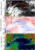 |
Fig. 6 Similar to Fig. 4, but for the third raster scan in the self-helicity phase. The dotted lines highlight the Si IV loops, the vertical dashed lines indicate the position of the spectra, now shown in Fig. 7. Same FOV as in Fig. 4. |
4.2. Self-helicity in a loop
The most significant change from the earlier mutual-helicity phase is found in the spectral profiles of Si IV. To illustrate this, we show in Fig. 7 the spectral images at several slit positions, labeled a to i in Fig. 6. In the middle part of loop 1 (red markers) the Si IV line shows a clear spectral tilt from positions e through h (Figs. 7e−f). Toward the left and right footpoints the spectra show no such spectral tilts.
The spectral tilt in the middle part of the loop is very clear, and the centroid of the profile changes from red to blue across a few pixels within the clearly defined cool loop. From Figs. 7e to h, one can estimate the spectral tilt from about 10 km s-1 blueshift on the southern side to about 30 km s-1 on the northern side. This is a signature of internal helical motions and indicates that loop 1 now has self-helicity (e.g., the twist). The profiles of the Mg II line show a similar spectral tilt, but here with weaker Doppler shifts than in Si IV (see Appendix A and Fig. A.4 for details).
In summary, this is evidence that the mutual helicity of the two loops turned into the internal helicity of a single loop.
4.3. Pitch angle of the flow
From the images and spectra observed by IRIS, we can estimate the real plasma motions along loop 1 during the self-helicity phase. The apparent velocity of the proper motion along loop 1 in the self-helicity phase is about 30 km s-1 (Fig. 3c and Sect. 4.1). The spectral tilt across loop 1 is of about 40 km s-1 (Figs. 7e to h and Sect. 4.2). From this one can estimate that the pitch angle of the internal helical motion is of about 20° to 45°. Consequently, the speed of the helical motion is about 40 km s-1, which is close to the sound speed of about 50 km s-1 near 100 000 K in the line formation region of Si IV.
5. Discussion and conclusions
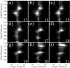 |
Fig. 7 Similar to Fig. 5, but for the self-helicity phase, now showing Si IV (1403 Å). The red and green markers show the position of the loops indicated by red and green dotted lines in Fig. 6a. |
In an observation with IRIS we found two cool loops with mutual helicity that interact. In this process the mutual helicity is transformed into self-helicity. Images acquired with AIA/SDO support that cool structures are present in the mutual-helicity phase, which are then heated by the interaction of the loops. The spectroscopic observations with IRIS clarify that the cool loops wind around each other and produce an increased line broadening due to the interaction and heating at the location of the loop crossing. The spectral tilt of the spectra within the single remaining full cool loop is a clear indication for the conversion of mutual into self-helicity. The pitch angle of the final internal helical motion in that loop is about 20° to 45°, the average velocity is about 30 km s-1 to 45 km s-1. The filament-type structures in the 304 Å channel of AIA are consistent with the mutual and self-helicity in filaments (Chae 2000). The bright dots in the AIA 171 Å channel might be indicative of hot plasma that is driven away from the interaction site.
Our investigation of the loops in Mg II k showed results similar to those for Si IV, albeit less clearly. This implies that these loops are multithermal: first, the Mg II intensity shows loops that are roughly co-spatial with those in Si IV. Second, and more important, the spectral profiles of Mg II and Si IV show similar characteristics at the location of the loops. Therefore it is highly unlikely that what we see in Mg II is just some low-lying plasma along the line of sight. Instead, the source region of Mg II has to be the same volume as the source region of Si IV. Thus the loops we studied contain chromospheric and transition-region plasma.
Tilts of spectral lines have been observed before and have been interpreted as rotational or twisting motions (e.g., Pasachoff et al. 1968; Rompolt 1975; Curdt et al. 2012; De Pontieu et al. 2012). Recent IRIS observations showed that these twisting motions are a ubiquitous phenomenon on the Sun (De Pontieu et al. 2014b). The random faint short-lived spectral tilts during the mutual-helicity phase are similar to the ubiquitous propagating twists along chromospheric features reported by De Pontieu et al. (2014b), which are signatures of self-helicity-driven spicule-like features. It has been proposed before that the conversion from mutual into self-helicity might occur when two crossing loops interact through reconnection (Berger 1999; Georgoulis 2011; Tziotziou et al. 2013). However, direct observational evidence for this conversion process could not be found. The new IRIS observations presented here allow following this conversion process and thus provide a new insight into how loops with internal twists might form. In the self-helicity phase the spectral tilt is distributed along the loop and is not only concentrated at the crossing point of the two loops. This indicates that the self-helicity propagates away from the magnetic reconnection site. Unfortunately, the current data do not allow following the temporal evolution of the self-helicity signatures, which one might naively expect to propagate with the Alfvén speed.
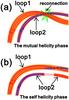 |
Fig. 8 Schematic diagrams illustrating the configurations of two loops, the orange-colored broad lines of loop 1 and loop 2, during the mutual helicity a) and the self-helicity phases b). The red lines in a) show the magnetic field lines of loop 1, the blue lines show the field lines of loop 2. The green star denotes magnetic reconnection. The red-blue lines in b) indicate the reconnected lines,the dotted red lines show loops that are not detected in Si IV images. The red and blue arrows show the directions of the magnetic field lines. |
The scenario for the conversion of mutual into self-helicity is sketched in Fig. 8. Here we interpret the conversion as interchange reconnection between the two crossing loops. The blue and red lines show the magnetic field lines, the more diffuse orange-colored broad lines represent the actual cool loops as seen in the 1400 Å channel of IRIS. In the mutual-helicity phase the red fieldlines fully belong to loop 1, the blue fieldlines fully to loop 2 (Fig. 8a): the loops wind around each other, which is the same as to say as that they have mutual helicity. At the crossing point reconnection sets in (green star), which marks the beginning of the end of the mutual-helicity phase. After the reconnection there are again two loops, but now more or less running in parallel with some of the fieldlines exchanged. The upper of the two loops in this later stage is now internally twisted within itself, which is a consequence of the interchange reconnection: now loop 1has self-helicity. Flows are initiated during the reconnection process, and as they move along the loop with self-helicity, they
show a twisting motion, which is detectable in the observations as a spectral tilt. In the end, this schematic diagram is similar to the process in which helical flux ropes are produced by reconnection (e.g., Moore et al. 2001; Cheng et al. 2014). Using Hi-C observations, Cirtain et al. (2013) showed evidence of braiding, subsequent reconnection, and straightening of the loops in the corona. Their scenario is similar to what we displayed in Fig. 8, but for multiset loops. However, our additional spectral data enable us to identify line-of-sight motions of, and even the motions inside, the unresolved loop strands. The IRIS observations presented here show a direct observational signature of this scenario of a conversion of mutual into self-helicity.
Online material
Movie of Fig. 1 Access here
Appendix A: Chromospheric observations of mutual- and self-helicity in the two loops
To relate the transition region plasma to emission from chromospheric origin, we analyzed the Mg II k (2796 Å) line of these two loops observed by IRIS in the same way as for the Si IV data shown in the main part of this study.
Figure A.1 displays the loops during the second scan in the mutual-helicity phase. Figure A.1b shows the intensity of the Mg II line. Two fainter loops are detected (roughly) co-spatially with the Si IV loops, as displayed in Fig. A.1a (see also Fig. 4a). This applies especially to the region surrounding the middle part of these two loops, which is marked by two red arrows.
The yellows crosses in the two panels of Fig. A.1 are at exactly the same positions. The alignment between the Si IV and Mg II maps is easily achieved using the fiducial marks on the slit that are visible in the spectro-heliograms as horizontal black lines. The yellow crosses mark two positions along the Si IV loops, and a comparison of panel a and b of Fig. A.1 shows that the loops of the Mg II k line are located ~1′′ to the south of the Si IV loops. Thus the chromospheric and transition region plasma is not at exactly the same position, but they most likely populate different strands of the same loop system.
Figure A.2 displays the profiles of Mg II k at 2796 Å in the mutual-helicity phase. The positions of the spectra are the same as those of the Si IV profiles shown in Fig. 5. The red and green marks here indicate the positions of the Si IV loops as displayed in Fig. 5. By comparing Fig. A.2 with Fig. 5, we can find some similar indications of the Doppler motions of the loops, even though the signals are weaker in the Mg II k line.
Figure A.3 shows the loops during the third scan in the self-helicity phase. Here, again, the Mg II line shows roughly the same loop patterns. Just as in the earlier mutual-helicity phase, here the loops seen in Mg II seem to be offset by ~1′′ to the south of the Si IV loops (because the FOV is different in this raster-scan map, the fiducial mark is not visible in Fig. A.3).
In Fig. A.4 we show the spectra of Mg II now in the self-helicity phase, again at the same positions as those of Si IV in the main text (cf. Fig. 7). For the north loop, loop 1, some spectral tilt is detected (see Figs. A.4e−h). These spectral tilts are similar to those displayed in Fig. 7 for Si IV, but with weaker Doppler shifts.
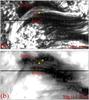 |
Fig. A.1 Intensity maps of IRIS Si IV (1394 Å) a) and Mg II k (2796 Å) b) during the second scan in the mutual-helicity phase. The yellow pluses mark the positions of the Si IV loops. The FOV is the same as in Fig. 4a. |
From these considerations we conclude that the spectro-heliograms in Mg II show loop structures similar to those in Si IV, albeit offset by about 1′′ perpendicular to the loop spine. Most importantly, even the spectral profiles of Mg II and Si IV share similar properties. This implies that the source region of the chromospheric Mg II k line and the transition region line of Si IV share the same volume defined by the loop system. Thus the loops are indeed multithermal structures, probably with the chromospheric and transition region plasma found on different strands within the loop system. However, because the signals in the Mg II k line are much weaker than in the Si IV line, the results we discussed here need to be considered carefully.
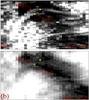 |
Fig. A.3 Same as Fig. A.1, but for the self-helicity phase, now showing the Si IV (1403 Å) a) and Mg II k (2796 Å) line b). |
The IRIS data are available at http://iris.lmsal.com/data.html
We cannot fully rule out that the emission in the AIA 171 Å band is due to cool plasma because this channel shows some contamination from O V lines. However, based on the temporal evolution we do not consider this likely, because then the early part of the mutual-helicity phase of the 171 Å channel should have shown the loops when they were already clearly visible in the transition region emission in Si IV.
Acknowledgments
IRIS is a NASA Small Explorer mission developed and operated by LMSAL with mission operations executed at NASA Ames Research center and major contributions to downlink communications funded by the Norwegian Space Center (NSC, Norway) through an ESA PRODEX contract. This work is supported by NASA contract NNG09FA40C (IRIS), the Lockheed Martin Independent Research Program, the European Research Council grant agreement No. 291058 and NASA grant NNX11AO98G. The AIA and HMI data used are provided courtesy of NASA/SDO and the AIA and HMI science teams. This work is supported by the National Basic Research Program of China under grant 2011CB811403, the National Natural Science Foundations of China (11303050, 11025315, 11221063) and the CAS Project KJCX2-EW-T07.
References
- Berger, M. A. 1999, in Magnetic Helicity in Space and Laboratory Plasmas, eds. M. R. Brown, R. C. Canfield, & A. A. Pevtsov, 1 [Google Scholar]
- Chae, J. C. 2000, ApJ, 540, L115 [NASA ADS] [CrossRef] [Google Scholar]
- Cheng, X., Ding, M. D., Zhang, J., et al. 2014, ApJ, 789, 93 [NASA ADS] [CrossRef] [Google Scholar]
- Cirtain, J., Golub, L., Winebarger, A., et al. 2013, Nature, 493, 501 [NASA ADS] [CrossRef] [Google Scholar]
- Cook, J. W., Bruechner, G. E., Bartoe, J.-D., & Socker, D. G. 1984, Adv. Space Res., 4, 59 [NASA ADS] [CrossRef] [PubMed] [Google Scholar]
- Curdt, W., & Tian, H. 2011, A&A, 532, L9 [NASA ADS] [CrossRef] [EDP Sciences] [Google Scholar]
- Curdt, W., Tian, H., & Kamio, S. 2012, Sol. Phys., 280, 417 [NASA ADS] [CrossRef] [Google Scholar]
- De Pontieu, B., Carlsson, M., Rouppe van der Voort, L. H. M., et al. 2012, ApJ, 752, L12 [NASA ADS] [CrossRef] [Google Scholar]
- De Pontieu, B., Title, A. M., Lemen, J. R., et al. 2014a, Sol. Phys., 289, 2733 [NASA ADS] [CrossRef] [Google Scholar]
- De Pontieu, B., et al. 2014b, Science, submitted [Google Scholar]
- Georgoulis, M. K. 2011, in The Physics of Sun and Star Spots, eds. D. P. Choudhary, & K. G. Strassmeier (Cambridge: Cambridge Univ. Press), IAU Symp., 273, 495 [Google Scholar]
- Kamio, S., Curdt, W., Teriaca, L., Inhester, B., & Solanki, S. 2010, A&A, 510, L1 [NASA ADS] [CrossRef] [EDP Sciences] [Google Scholar]
- Lemen, J. R., Title, A. M., Akin, D. J., et al. 2012, Sol. Phys., 275, 17 [NASA ADS] [CrossRef] [Google Scholar]
- Moore, R. L., Sterling, A. C., Hudson, H. S., & Lemen, J. R. 2001, ApJ, 552, 833 [NASA ADS] [CrossRef] [Google Scholar]
- Orozco Suárez, D., Asensio Ramos, A., & Trujillo Bueno, J. 2012, ApJ, 761, L25 [NASA ADS] [CrossRef] [Google Scholar]
- Pasachoff, J.-M., Noyes, R. W., & Beckers, J. M. 1968, Sol. Phys., 5, 131 [NASA ADS] [CrossRef] [Google Scholar]
- Pesnell, W. D., Thompson, B. J., & Chamberlin, P. C. 2012, Sol. Phys., 275, 3 [NASA ADS] [CrossRef] [Google Scholar]
- Pike, C. D., & Mason, H. E. 1998, Sol. Phys., 182, 333 [NASA ADS] [CrossRef] [Google Scholar]
- Régnier, S., Amari, T., & Canfield, R. C. 2005, A&A, 442, 345 [NASA ADS] [CrossRef] [EDP Sciences] [Google Scholar]
- Rompolt, B. 1975, Sol. Phys., 41, 329 [NASA ADS] [CrossRef] [Google Scholar]
- Schou, J., Scherrer, P. H., Bush, R. I., et al. 2012, Sol. Phys., 275, 229 [Google Scholar]
- Su, Y., Gömöry, P., Veronig, A., et al. 2014, ApJ, 785, L2 [NASA ADS] [CrossRef] [Google Scholar]
- Tian, H., Curdt, W., Marsch, E., & He, J. S. 2008, ApJ, 681, L121 [Google Scholar]
- Tziotziou, K., Georgoulis, M. K., & Liu, Y. 2013, ApJ, 772, 115 [NASA ADS] [CrossRef] [Google Scholar]
- Wedemeyer, S., Scullion, E., Rouppe van der Voort, L., et al. 2013, ApJ, 774, 123 [NASA ADS] [CrossRef] [Google Scholar]
All Tables
All Figures
|
Fig. 1 IRIS slit-jaw images and context from AIA and HMI. The left panels a)−c) show snapshots of the IRIS slit-jaw images during the three raster scans. The right panels show the SDO context: the AIA 304 Å image d) and the HMI LOS magnetogram e) during the first scan, and the AIA 171 Å image f) during the third scan. The yellow dotted lines in panels a) and d) outline the envelope containing the two cool loops seen in the IRIS slit-jaw images. The red circles mark the endpoints of these loops. The green arrows in a) and b) indicate the crossing point. The red dashed lines in b) and c) show the positions for time-space diagrams displayed in Fig. 3. The green rectangles in b) and c) are the FOV of Figs. 4 and 6. The center of this image is at solar (x,y) = (319″,102″), and the FOV is 75″ × 50″. The temporal evolution of the IRIS slit-jaw images at 1400 Å of the AIA 304 Å and 171 Å channels the HMI magnetograms is available in the online edition. |
| In the text | |
|
Fig. 2 Line profiles used for wavelength calibration averaged over the whole FOV of the raster map. Panels a) and b) show the profile during the second raster. The main target line Si IV at 1394 Å is visible in a). The vertical dotted lines indicate the wavelength region shown in panel b), where we zoom in on the lines of Ni II and Fe II that were used for wavelength calibration. The pluses show the actual observed spectrum, the solid line a spline fit around the center of the calibration lines. The vertical dashed lines indicate the peak of the spline fit. Panels c) and d) show the same for the third raster scan in the self-helicity phase. Here the S I line was used for wavelength calibration and the main target line was Si IV at 1403 Å. The count rate is per 0.166′′×0.166′′ pixel. |
| In the text | |
|
Fig. 3 Proper motions along the Si IV loops. Time-space plots of a series of IRIS slit-jaw images at 1400 Å along the dashed lines AB a), CD b), EF c), and GH d), as marked in Figs. 1b and c. The red dashed lines show motions along the loops. The respective velocities are denoted by the numbers in the plots. |
| In the text | |
|
Fig. 4 Maps of intensity a), Doppler shift b), and line width c) of Si IV (1394 Å) for the second raster scan in the mutual-helicity phase. The dotted lines highlight the location of the two cool loops. The dashed lines a−i in a) and b) indicate the positions of the spectra shown in Fig. 5. The yellow arrow in c) marks a region with enhanced line width. The location of the maps is indicated in Fig. 1b. The FOV is 60.5″ × 33.3″. |
| In the text | |
|
Fig. 5 Line profiles of Si IV (1394 Å) during the mutual-helicity phase. The spatial location of these spectra is indicated in Fig. 4 by the vertical dashed lines a−i. The red and green markers show the location of the two loops (red and green dotted lines in Fig. 4a). The numbers in the plot indicate the raster index, the vertical dotted lines the zero Doppler shift. |
| In the text | |
|
Fig. 6 Similar to Fig. 4, but for the third raster scan in the self-helicity phase. The dotted lines highlight the Si IV loops, the vertical dashed lines indicate the position of the spectra, now shown in Fig. 7. Same FOV as in Fig. 4. |
| In the text | |
|
Fig. 7 Similar to Fig. 5, but for the self-helicity phase, now showing Si IV (1403 Å). The red and green markers show the position of the loops indicated by red and green dotted lines in Fig. 6a. |
| In the text | |
|
Fig. 8 Schematic diagrams illustrating the configurations of two loops, the orange-colored broad lines of loop 1 and loop 2, during the mutual helicity a) and the self-helicity phases b). The red lines in a) show the magnetic field lines of loop 1, the blue lines show the field lines of loop 2. The green star denotes magnetic reconnection. The red-blue lines in b) indicate the reconnected lines,the dotted red lines show loops that are not detected in Si IV images. The red and blue arrows show the directions of the magnetic field lines. |
| In the text | |
|
Fig. A.1 Intensity maps of IRIS Si IV (1394 Å) a) and Mg II k (2796 Å) b) during the second scan in the mutual-helicity phase. The yellow pluses mark the positions of the Si IV loops. The FOV is the same as in Fig. 4a. |
| In the text | |
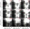 |
Fig. A.2 Similar as Fig. 5, but for the Mg II k (2796 Å) line. |
| In the text | |
|
Fig. A.3 Same as Fig. A.1, but for the self-helicity phase, now showing the Si IV (1403 Å) a) and Mg II k (2796 Å) line b). |
| In the text | |
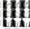 |
Fig. A.4 Same as Fig. A.2, but for the self-helicity phase. |
| In the text | |
Current usage metrics show cumulative count of Article Views (full-text article views including HTML views, PDF and ePub downloads, according to the available data) and Abstracts Views on Vision4Press platform.
Data correspond to usage on the plateform after 2015. The current usage metrics is available 48-96 hours after online publication and is updated daily on week days.
Initial download of the metrics may take a while.