| Issue |
A&A
Volume 568, August 2014
|
|
|---|---|---|
| Article Number | A85 | |
| Number of page(s) | 10 | |
| Section | Galactic structure, stellar clusters and populations | |
| DOI | https://doi.org/10.1051/0004-6361/201423991 | |
| Published online | 22 August 2014 | |
GCIRS 7, a pulsating M1 supergiant at the Galactic centre
Physical properties and age⋆,⋆⋆
1 LESIA, Observatoire de Paris, CNRS, UPMC, Université Paris-Diderot, PSL research university, 5 place Jules Janssen, 92195 Meudon, France
e-mail: thibaut.paumard@obspm.fr
2 Max-Planck-Institut für extraterrestrische Physik, 85748 Garching, Germany
e-mail: pfuhl@mpe.mpg.de
3 LUPM, Université Montpelier 2, CNRS, Place Eugène Bataillon, 34095 Montpellier, France
4 Max-Planck-Institut für Astronomie, Königstuhl 17, 69117 Heidelberg, Germany
5 Univ. Grenoble Alpes, IPAG, 38000 Grenoble, France CNRS, IPAG, 38000 Grenoble, France
6 European Southern Observatory, Alonso de Córdova 3107, Casilla 19001, Santiago 19, Chile
Received: 14 April 2014
Accepted: 19 June 2014
Context. The stellar population in the central parsec of the Galaxy is dominated in mass and number by an old (several Gyr) population, but young (6 ± 2 Myr), massive stars dominate the luminosity function. The most luminous of these stars is an M1 supergiant, GCIRS 7.
Aims. We have studied GCIRS 7 in order to constrain the age of the recent star formation event in the Galactic centre and to characterise it as a visibility and phase reference for observations of the Galactic centre with the interferometric instrument GRAVITY, which will equip the Very Large Telescope Interferometer (VLTI) in the near future.
Methods. We present the first H-band interferometric observations of GCIRS 7, obtained using the PIONIER visitor instrument on the VLTI using the four 8.2-m unit telescopes. In addition, we present unpublished K-band VLTI/AMBER data and build JHKL light curves based on archival data spanning almost 40 years, and measured the star’s effective temperature using SINFONI integral field spectroscopy.
Results. GCIRS 7 is marginally resolved in the H band with a uniform-disk diameter θUD(2013) = 1.076 ± 0.093 mas (RUD(2013) = 960 ± 92 R⊙ at 8.33 ± 0.35 kpc). We detect a significant circumstellar contribution in the K band. The star and its environment are variable in brightness and in size. The photospheric H-band variations are modelled well with two periods: P0 ≃ 470 ± 10 days (amplitude ≃0.64 mag) and long secondary period PLSP ≃ 2700 − 2850 days (amplitude ≃1.1 mag). As measured from 12CO equivalent width, ⟨Teff⟩ = 3600 ± 195 K.
Conclusions. The size, periods, luminosity (⟨Mbol⟩ = −8.44 ± 0.22), and effective temperature are consistent with an M1 supergiant with an initial mass of 22.5 ± 2.5 M⊙ and an age of 6.5–10 Myr (depending on rotation). This age is in remarkable agreement with most estimates for the recent star formation event in the central parsec. Caution should be taken when using this star as a phase reference or visibility calibrator because it is variable in size, is surrounded by a variable circumstellar environment, and large convection cells may form on its photosphere.
Key words: Galaxy: nucleus / supergiants / stars: individual: / techniques: interferometric / techniques: photometric / techniques: spectroscopic
This work relies on interferometric, spectroscopic, and imaging data obtained at the VLT and VLTI in Cerro Paranal Chile between 2003 and 2013. The observations were carried out under the programme IDs 075.B-0547, 076.B-0259, 077.B-0503, 179.B-0261, 381.D-0529, 183.B-0100, 087.B-0117, 087.B-0280, 088.B-0308, 288.B-5040, and 091.D-0682.
© ESO, 2014
1. Introduction
The central parsec of the Milky Way galaxy is host to a dense star cluster that is made of a relaxed population of late-type stars intermixed with a much younger population of luminous, evolved, massive stars (Genzel et al. 2010, and references therein). About one hundred of those young stars seem to have been born in one single event of star formation, presumably within a massive self-gravitating accretion disk that is hypothesised to have existed at that time around the super-massive black-hole candidate Sgr A* (Paumard et al. 2006; Bartko et al. 2009; Lu et al. 2013, and references therein).
GCIRS 7 is by far the brightest star in the Galactic centre (GC) in the H and K bands. This M1 supergiant (Blum et al. 1996b) has been first observed in 1966 by Becklin & Neugebauer (1968, 1975). Interstellar medium (ISM) features north of the source are interpreted as the outer layers of the star’s atmosphere being blown away by the central cluster wind in a cometary tail (Serabyn et al. 1991; Yusef-Zadeh & Morris 1991). This star is in itself an interesting target: it is the brightest of the very few current-day red supergiant (RSG) stars presumably formed together with the disk of young stars in the GC (Krabbe et al. 1995). It also interacts with a wind from either the hot stars or perhaps the black-hole vicinity itself.
In addition, GCIRS 7 is an important star for future observations in the GC. It has often been used as wave-front reference for infrared adaptive optics systems such as NAOS, and will be used again for that purpose for interferometric observations with the 4-telescope beam combiner GRAVITY (Eisenhauer et al. 2008). It will also very likely be used as a fringe-tracker and phase reference for certain GC observations involving the 1.8-m auxiliary telescopes (ATs). It is therefore timely to study its interferometric structure and behaviour.
Pott et al. (2008) have observed the star using AMBER in the K band and MIDI in the N band. They find that the star is marginally resolved in the K band, more so than its photospheric luminosity would suggest, and strongly resolved in the N band. They conclude that dust surrounding the star dominates the visibility in the mid-infrared and has a non-negligible contribution in the near-infrared.
Blum et al. (1996a) have shown that the luminosity of GCIRS 7 has increased by approximately 0.8, 0.5, and 0.3 mag in the J,H, and K band, respectively, between 1978 and 1993. Ott et al. (1999) have measured a K-band luminosity decrease of 0.7 mag between 1992 and 1998. Those authors have not been able to determine any particular regularity in the light curve and have classified GCIRS 7 as a long-period variable (LPV) supergiant.
In Sect. 2, we describe our original and archival data sets. In Sect. 2.3, we derive stellar parameters such as the size, the effective temperature, interferometric and photometric variations, the age, and the mass of the star (Table 1). We discuss our findings in Sect. 4.
2. Observations
Physical parameters.
2.1. Interferometry
2.1.1. PIONIER 2013
We observed the star using PIONIER (Le Bouquin et al. 2011) using the four 8.2 m Unit Telescopes (UTs) of the VLTI on July 18 and 21, 2013. We used an optical wave-front reference star about 15” north–east of the target (USNO-A2.0 0600-28577051). The (u,v) coverage is shown in Fig. 1. Since we wanted to observe fairly faint targets with off-axis adaptive optics, we used the H-band undispersed mode of the instrument.
The atmospheric conditions on the first night were partly cloudy with a fast coherence time (≃3 ms). We were nevertheless able to record fringes on all six baselines (Fig. 2) and to observe a good set of calibration stars. The second night was clearer, but the coherence time was even shorter (≃1 ms) so that it proved impossible to stabilise the fringes, which we were able to witness by eye, on the detector. We therefore searched for fringes on a brighter calibrator and then trusted the VLTI delay line model to apply the right offsets when pointing GCIRS 7. We then recorded scans blindly on the source. Indeed, several scans proved usable at data reduction time and confirmed the visibilities measured on the first night.
The data were reduced using the version 2.55 of the PIONIER pipeline pndrs (Le Bouquin et al. 2011). Since our target is at rather low signal-to-noise, and in order not to introduce biases, we decided to select scans where fringe detection is certain from a visual inspection of the scan waterfalls, but not to filter more within those scans because additional filtering may lead to biases.
In total, we have been able to obtain data for all six baselines on the first night and only for U1–U2 and U1–U3 (not at the same time) on the second night (Fig. 3). Closure phases were also measured on all three triplets on the first night, all compatible with 0° to within the uncertainties, as expected for an unresolved or marginally resolved source.
2.1.2. AMBER 2008
GCIRS 7 and the calibrator were observed with AMBER in low-resolution mode and a frame exposure time (DIT) of 50 ms, on the night of May 17, 2008 with the VLTI-UT sub-array UT134. Fringes were recorded on all three baselines in service mode operation. The (u,v) coverage is shown in Fig. 1. Seeing was typically better than 1′′. Adaptive optics guiding with MACAO was performed using the same reference star as during our PIONIER observations (USNO-A2.0 0600-28577051). The visibility calibrator HD 164866 (mK = 6.5 mag) was observed close to the target (dist = 4.6°).
The data were reduced following standard procedures as described in Tatulli et al. (2007) and Chelli et al. (2009), using the amdlib package, release 3.0.8, and the yorick interface provided by the Jean-Marie Mariotti Centre (JMMC)1. First, raw spectral visibilities and closure phases were extracted for all the frames of each observing file. Then a selection of frames with a piston smaller than 15 μm was made to achieve a higher signal-to-noise ratio (S/N) on the visibilities and phases. GCIRS 7 was at the very limit of sensitivity of AMBER in 2008. Therefore we confirmed getting stable, calibrated results with two S/N-based frame selections (20%, Fig. 4, and 80%). The two frame selections within the piston-limited subset yield the same results within the stated uncertainties, which is reassuring. The transfer function was obtained by averaging the calibrator measurements, after correcting for their intrinsic diameters. Here again, closure phases are statistically compatible with 0°.
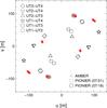 |
Fig. 1 Projected baselines ((u,v) coverage) of the PIONIER (large symbols) and AMBER (small symbols) data. |
 |
Fig. 2 Example fringe waterfalls for one exposure. Each panel corresponds to one telescope pair. In each panel, the vertical axis corresponds to scan number (one scan lasts ≃1 s) and the horizontal axis to index within scan (which corresponds to optical path difference). In this specific example, fringes are present on all baselines. |
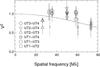 |
Fig. 3 2013 H-band PIONIER data, V2 vs. spatial frequency in 106/rad or Mλ. Solid line: uniform-disk model of diameter 1.076 mas. Larger black symbols: first night, smaller grey symbols: second night. |
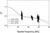 |
Fig. 4 2008 K-band AMBER data, V2 vs. spatial frequency in 106/rad or Mλ. Lines: several two-component models where the star is represented by a uniform disk and the environment by: solid line: a circle, representing a thin shell; dashed line: a second uniform disk, representing a thick shell; dash-dotted line: a uniform background. |
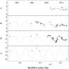 |
Fig. 5 J,H,Ks, and L-band light curves. The oldest data is from 1975, the latest from June 2013. Statistical uncertainties are represented, although they are often smaller than the symbol. Diamonds: NACO data; squares: from Peeples et al. (2007); circles: from Ott et al. (1999, these points have been brought up by 0.3 mag); triangles: from Blum et al. (1996a) which includes data from Becklin & Neugebauer (1975) and Depoy & Sharp (1991). Dashed curves: sinusoidal models with a period of 2850 d. |
2.2. Photometry
2.2.1. NACO imaging photometry
The photometric data were obtained with the adaptive optics camera NACO (Rousset et al. 2003; Lenzen et al. 2003). The images were taken between 2002 and 2013. Most of the images were taken with the H and Ks-band filters with the 13 mas/pixel or the 27 mas/pixel camera. Additional L-band images and one J-band one were obtained with the 27 mas/pixel camera. Especially the H and Ks-band images were selected depending on the saturation level of GCIRS 7 in the image. Images with very good seeing and long integration times had to be removed because they were strongly affected by saturation. Each selected image was sky-subtracted, as well as bad-pixel- and flat-field-corrected. In total we used 20 Ks-band, 39 H-band, 21 L-band, and one J-band image with temporal spacing between one day and up to 11 years to construct the light-curve of GCIRS 7.
The photometry on the individual images was done by 2D Gaussian fits to the stars. As photometric references, the bright early-type stars GCIRS 16NE and GCIRS 16C were used. Both stars showed little or no variability over the recorded time base. We used the magnitudes stated by Blum et al. (1996a) as reference magnitudes (GCIRS 16NE: mJ = 14.01 ± 0.08, mH = 10.94 ± 0.08, mKs = 9.01 ± 0.05, and mL = 7.56 ± 0.09; GCIRS 16C: mJ = 15.20 ± 0.08, mH = 11.96 ± 0.08, mKs = 9.83 ± 0.05, and mL = 8.48 ± 0.10).
2.2.2. Archival photometry
The star GCIRS 7 is the brightest individual source in the vicinity of Sgr A* in the near infrared. As such the star was targeted in many photometric surveys during the last decades. In an attempt to get a light curve as long and complete as possible, we used all published J,H,Ks and L-band data that we were aware of. This includes data from Becklin & Neugebauer (1975), Depoy & Sharp (1991), Ott et al. (1999), Blum et al. (1996a), and Peeples et al. (2007). By comparing various stars (most notably GCIRS 16NE and 16C) in the published data sets (in particular Blum et al. 1996a), it turned out that the K-band data from Ott et al. (1999) seemed to be offset (brighter) on average by about 0.3 Mag. This could be related to the choice of the magnitude reference star. To account for this difference, we added 0.3 mag to the Ott et al. magnitudes. The combined light curve is shown in Fig. 5.
2.3. SINFONI spectroscopy
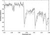 |
Fig. 6 SINFONI spectra. Only the three spectra with a resolution of ≃2000 are shown. Dark gray: MJD = 52 738; black: MJD = 55 383; light grey: MJD = 56 558. |
Our spectroscopic data (Fig. 6) were obtained with the adaptive-optics-assisted integral field spectrograph SINFONI (Eisenhauer et al. 2003; Bonnet et al. 2004). In total we used four observations obtained in April 2003 (MJD = 52 738), August 2004 (MJD = 53 237), July 2010 (MJD = 55 383), and September 2013 (MJD = 56 558) with pixel scales between 50 × 100 and 125 × 250 Mas. The data output of SINFONI consists of cubes with two spatial axes and one spectral axis. Depending on the plate scale, an individual cube covers 3.2″ × 3.2″ or 8″ × 8″ and the spectral resolving power was about 2000 except for the 2004 run (R ≃ 4000). We used the data reduction SPRED (Schreiber et al. 2004; Abuter et al. 2006), including bad-pixel correction, flat-fielding, and sky subtraction. The wavelength scale was calibrated with emission line gas lamps and fine-tuned on the atmospheric OH lines. Finally we removed the atmospheric absorption features by dividing the spectra through a telluric spectrum obtained each respective night.
3. Results
The various physical parameters derived below, as well as a few complementary parameters from the literature, are summarised in Table 1.
3.1. Size
The H-band 2013 visibilities remain very high for spatial frequencies below 60 Mλ (i.e. B⊥/λ< 6 × 10⁷ where B⊥ is the projected baseline length), except on the shortest baseline (U2–U3), for which the data have the lowest S/N. A decrease above 60 Mλ (B⊥> 100 m at λ = 1.68μm) is observed on the first night on the longest baseline (U2–U3), which also has a fairly low S/N, and on the second night on U1–U3. At any rate, V2 ≳ 0.7 even at 73 Mλ. This points towards a barely resolved source.
Indeed, the best-fit uniform-disk diameter is only θUD = 1.076 ± 0.093 mas, corresponding to RUD ≃ 960 ± 92 R⊙ at 8.33 ± 0.35 kpc. To estimate a limb-darkened diameter, we used the law of Claret (2000) and the coefficients for Teff = 3500 K, log (g) = 0, solar metallicity. The fitted value (4% higher than θUD, as expected) is the same within the statistical uncertainties: θLD = 1.116 ± 0.098mas. In both cases, the reduced χ2 is about 1.9. The stated error bars are rescaled to account for the imperfect fits. The reduced χ2 for θUD = 0 (resp. 2) mas is ≃4 (resp. 9). Again, this shows that the source is only moderately resolved.
On the other hand, the K-band 2008 visibilities are V2 ≃ 0.5 for all baselines. This is a strong indication that up to 30% of the flux comes from a resolved environment, while ≳70% comes from a compact source. We fitted a few models where the star is represented by a uniform disk and the environment is represented by a ring, a second uniform disk, or a uniform background. In all cases, the photospheric size is in the range θUD1.5–2 mas (RUD = 1340–1790 R⊙), the diameter of the circumstellar component is >5 mas, and the star accounts for 75–85% of the flux. These values should be considered with caution, though, because the (u,v) coverage is not sufficient, given the uncertainties, to characterise both the stellar photosphere and the environment in detail.
3.2. Light curve periodicities
Figure 5 shows the photometric data described in Sects. 2.2.1 and 2.2.2. GCIRS 7 is clearly variable at J to L-band, as noted before in the literature. Our PIONIER H-band observations (modified Julian date MJD ≃ 56 490) as well as the 2006 AMBER observations presented in Pott et al. (2008, March 2006: MJD ≃ 53 800 occurred during a minimum of the star’s brightness. On the contrary, the AMBER K-band observations we present were acquired near a photometric maximum (MJD = 54 603). The H-band magnitude measured on one NACO frame in June 2013 (resp. June 2008) was mH(2013) ≃ 10.09 (resp. mH(2008) ≃ 9.21).
For the first time, we are able to show that GCIRS 7 is semi-periodic at least in the H band with a long-term period of ≃2850 days (7.8 yr). The H-band light curve samples the last two pseudo-periods very well, while Ott et al. (1999)K-band data cover the preceding period. The Becklin & Neugebauer (1975) data points are consistent with the extrapolated sine curves, while the Depoy & Sharp (1991) points (observed in 1989 and 1990) are too bright at all wavelengths.
The single periodicity sine-curve model is a fair representation of the light curve variations, but departures from this model are significant. In particular, shorter term variations are seen in the NACO data (Fig. 7). Furthermore, RSGs are known to often exhibit semi-periodic variations. Many stars show a short period (P0, of a few 100 days) which is explained well by the fundamental mode or first overtone of radial pulsation. Other stars show, in addition or instead, a longer period (PLSP> 1000 d) referred to as the long secondary period (LSP), which is not explained as well (see Kiss et al. 2006, and references therein).
Our time sampling is only good for the NACO era, and there it only extends for a little more than one period. We have constructed the generalised Lomb-Scargle periodograms (Fig. 8, Lomb 1976; Scargle 1982; Zechmeister & Kürster 2009) for the H-, K-, and L-band NACO data, which respectively contain data for 37, 20, and 13 distinct dates over 3641, 4142, and 4015 days, and attempted simple model fitting of one or two sine curves.
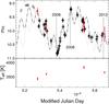 |
Fig. 7 Top: H-band light curve after year 2000. Bottom: effective temperature measurements from SINFONI spectra. Diamonds: NACO data (fitted); squares: Peeples et al. (2007, for comparison). Dash-dotted, dark grey curve: best-fit two-period model. Dotted, light grey curve: second best-fit model. Vertical lines: dates of interferometric observations: March 2006 (Pott et al. 2008, K-band AMBER), May 2008 (K-band AMBER) and July 2013 (H-band PIONIER). Crosses: Teff from SINFONI spectra and the corresponding magnitude estimated using the best fit model; the vertical line of each cross indicates only the statistical uncertainty (see text, Sect. 3.3). |
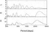 |
Fig. 8 Generalised Lomb-Scargle periodograms of the NACO light curves (bottom to top: H,K and L-band). Black curves: data periodograms. Light grey, dashed curve: single-period model. Dark grey, dash-dotted curve: two-period model. Vertical dotted lines: best fit periods. Vertical dashed lines: NACO time coverage in each band. The periodograms are normalised so that the expected power for pure Gaussian noise is 1. |
The χ2 map of the two-period model (Fig. 9) shows that there are only two pairs of periods able to reproduce the NACO data decently, fairly close to each other: (P0,PLSP) = (410 ± 10d,2120 ± 88d) and (470 ± 10,2620 ± 140). They cannot be distinguished using a χ2 argument alone. However, the second pair is closer to the longer term period seen in Fig. 5 and fits the Peeples et al. (2007) data points better (Fig. 7). This is therefore the solution we consider best. The seven best-fit parameters are listed in Table 2. The amplitudes associated with the two periods are in the same range: 0.6 ± 0.1 and 1.1 ± 0.1 mag peak-to-peak for the short and long periods, respectively. Although still not perfect (reduced χ2 = 4.7), this two-period model reproduces the data (Fig. 7) and their power spectrum (Fig. 8) much better than the single-period model (reduced χ2 = 10.4).
The K-band light curve from the NACO era almost appears to be constant at mK = 7, except the first point around mK = 6.5. The most prominent feature of the K-band periodogram is a broad peak, around 2800 d, which is compatible with both the long-term period (2850 d) and the short-term H-band PLSP (2620 d). We tried fitting one or two periods on the K-band data, as well as fitting only the amplitudes for two sine curves at the periods and phases determined from the H-band data. The reduced χ2 for the three different fits remains approximately the same. In conclusion, the K-band data favour PLSP ≃ 2800 d, are compatible with P0 obtained from the H-band data, but do not bring further constraints.
Finally, the L-band periodogram is dominated by a band of lines around 500 d, which could be the signature of P0 seen in the H-band data. The data sampling does not allow this to be firmly asserted, though.
3.3. Effective temperature
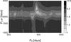 |
Fig. 9 χ2 map for the two-period H-band model, normalised to its minimum of 4.68. The best-fit period pairs are marked by uncertainty crosses. |
Best-fit parameters for the two-period model.
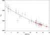 |
Fig. 10 CO-Teff calibration for RSGs with spectral types between G0 and M4. Open circles: stars from the IRTF library. The temperature uncertainty of the individual stars is 200 K (Allen & Cox 2000). Curve: best-fit empirical relation. Filled circles: EW(CO) measurements on GCIRS 7 and derived Teff. |
Cool stars with temperatures between 3000 K and 5000 K show prominent CO absorption features between 2.29 and 2.40 μm. The CO absorption strength varies sensitively with temperature, which makes the so-called CO band heads excellent tracers of the stellar temperature. Numerous definitions of the CO equivalent width have been proposed in the literature (e.g. Kleinmann & Hall 1986; Frogel et al. 2001). Previous studies of the cool stellar population in the GC such as Blum et al. (2003), Maness et al. (2007), and Pfuhl et al. (2011), determined accurate 12CO(2, 0)–Teff calibrations, but only for giant stars. The CO strength, however, depends not only on the effective temperature but also on surface gravity. Therefore to get reliable temperature estimates for the RSG GCIRS 7, it is necessary to determine an adequate 12CO(2, 0)–Teff calibration for RSGs.
To set such a calibration up, we used 34 published RSG spectra (R ≃ 2000) from the IRTF library (Rayner et al. 2009). The template spectra comprise stars with luminosity classes between Ia to Ib and spectral types between G0 and M4. We measured the CO strength according to the definition of Frogel et al. (2001) since their index proved to be insensitive to biases (Pfuhl et al. 2011). The effective temperature of the library stars was derived based on their spectral type. For spectral types between G0 and K0 we used temperatures from (Allen & Cox 2000, p. 152). For later spectral types K1 to M5, we used the revised calibration from Levesque et al. (2005). The result is shown Fig. 10. As expected, the CO strength clearly correlates with the stellar temperature. We used a second-order polynomial fit to get an empirical relation between EW(CO) and effective temperature. The best-fit relation is ![\begin{eqnarray} T_\text{eff} = 0.669 \cdot {\rm CO}^2 - 82.139 \cdot {\rm CO} +5414 \rm~[K]. \end{eqnarray}](/articles/aa/full_html/2014/08/aa23991-14/aa23991-14-eq154.png) (1)The intrinsic scatter of the template stars with respect to the best-fit temperature is 180 K. This is roughly consistent with the stated temperature uncertainty of the spectral types of ~200 K (Allen & Cox 2000, p. 153). All available temperature measurements are summarised in Table 3. Although the measurements used various techniques, they all agree very well. In the following, we use the mean of the measurements ⟨Teff⟩ = 3600 ± 195 K as an estimate of the average temperature of the star. The uncertainty is the mean of the individual uncertainties and is dominated by systematic errors. The root-mean-square scatter between the individual measurements is only 116 K.
(1)The intrinsic scatter of the template stars with respect to the best-fit temperature is 180 K. This is roughly consistent with the stated temperature uncertainty of the spectral types of ~200 K (Allen & Cox 2000, p. 153). All available temperature measurements are summarised in Table 3. Although the measurements used various techniques, they all agree very well. In the following, we use the mean of the measurements ⟨Teff⟩ = 3600 ± 195 K as an estimate of the average temperature of the star. The uncertainty is the mean of the individual uncertainties and is dominated by systematic errors. The root-mean-square scatter between the individual measurements is only 116 K.
Effective temperature of GCIRS 7.
Even though the systematic errors are too large to derive a consistent temperature curve, EW(CO) does change measurably between SINFONI runs (Fig. 10), and the colours also vary quite significantly. We investigate the temperature variations by only considering the statistical uncertainties in the four SINFONI Teff estimates, assuming that the systematic effects affect those four points in the same fashion. We also estimated the H-band magnitude of the star at the corresponding dates using our best fit model (Table 2). We used uncertainties on the fit parameters to derive uncertainties on these magnitudes. Those temperatures, magnitudes, and the corresponding uncertainties are shown Fig. 7.
To assess the significance of the variation in Teff between SINFONI runs, we first take the average of these four values: ⟨Teff⟩SINFONI = 3629 ± 18 K. The departure from this value for each date is −190 ± 46, −26 ± 36, 209 ± 49 and 32 ± 36 K. This is on average a 2.5σ departure.
3.4. Absolute magnitude and bolometric luminosity
The intrinsic K- and H-band luminosity of GCIRS 7 can be derived from the average observed ⟨mK⟩ = 6.8 ± 0.1 and ⟨mH⟩ = 9.93 ± 0.03, the measured K-band extinction AK = 3.48 ± 0.09 (Blum et al. 2003), AH/AK = 1.73 ± 0.03 (Nishiyama et al. 2009; Fritz 2013), and the distance modulus d = 14.6 ± 0.09 (assuming R0 = 8.33 ± 0.35 kpc, Gillessen et al. 2009). The absolute, dereddened K- and H-band magnitudes are therefore ⟨MK⟩ = −11.3 ± 0.16 and ⟨MH⟩ = −10.7 ± 0.2. The bolometric K-band correction for a star with Teff = 3600 ± 195 K is BCK = 2.84 ± 0.15 (Levesque et al. 2005). Thus the (average) absolute bolometric magnitude of GCIRS 7 is ⟨Mbol⟩ = −8.44 ± 0.22, corresponding to a luminosity of ⟨L⟩ = 1.86 ± 0.4 × 10⁵ L⊙. The position of GCIRS 7 in the Hertzsprung–Russell (HR) diagram can be seen in Fig. 11. Likewise, the 2013 values of the K- and H-band and bolometric absolute magnitudes are MK(2013) = −10.77 ± 0.15, MH(2013) = −10.52 ± 0.22, and Mbol(2013) = −7.93 ± 0.22, respectively.
To estimate the bolometric magnitude of the star at the time of the SINFONI observations, we lack a well-established H-band bolometric correction law. However, using Teff, mH, and the relations in Kervella et al. (2004), we can derive the radius of the star for these four epochs. From these radii and the temperatures, we can get the bolometric magnitude directly at each SINFONI observation. In this estimation, we are only interested in the statistical uncertainties and therefore do not consider the uncertainties on AK, AH/AK, and R0. The values are listed in Table 4.
3.5. Age and initial mass
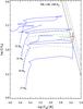 |
Fig. 11 Position of GCIRS 7 in the H-R diagram (cross) compared with evolutionary tracks of stars with initial masses between Mini = 15 − 32 M⊙ with rotation (blue solid) and for Mini = 20 − 25 M⊙ without rotation (dashed green) from Ekström et al. (2012). The solid black lines denote the theoretical luminosities of stars with radii of R = 900,1100, and 1300 R⊙ as a function of effective temperature. |
To estimate the initial mass and the age of GCIRS 7, we rely on the recent evolutionary tracks from Ekström et al. (2012, Fig. 11. Their tracks include stellar rotation and assume a solar metallicity. This seems to be a reasonable choice since GCIRS 7 is known to have a metallicity close to solar (Carr et al. 2000; Cunha et al. 2007). GCIRS 7 falls between the evolutionary tracks of Mini = 20 M⊙ and Mini = 25 M⊙ stars with and without rotation. Stars with initial masses of Mini = 20 M⊙ reach the RSG phase after about 8 Myr without rotation and 10 Myr with rotation and last there for about 0.2 Myr. Stars with initial masses of 25 M⊙ reach the RSG phase after about 6.5 Myr without and after 8 Myr with rotation and remain there for a few ten thousand years. Stars with initial masses of 15 M⊙ (RSG age 14–15 Myr) do not reach the observed luminosity. Unfortunately, evolutionary tracks with a finer mass sampling are available only through an interpolation tool2. GCIRS 7 lies on the far right end of the tracks, and the interpolation seems to cut some of this temperature extremum. The authors of the interpolation tools note that it cannot be relied upon for unstable phases. However, the available tracks (as well as the interpolated tracks) are roughly equally spaced in luminosity. Based on that we estimate that GCIRS 7 originates in a star with initial mass of 22.5 ± 2.5 M⊙ (in good agreement with Cunha et al. 2007, 22 M⊙). Depending on the initial rotation of the star, the age of GCIRS 7 is in the range 6.5–10 Myr.
Variations in Teff, MH, and RLD from the SINFONI spectra and NACO H-band photometry.
4. Discussion
4.1. Size of GCIRS 7 and its environment
The effective temperature and radius of 74 Galactic RSGs have been determined by van Belle et al. (2009). From their Eq. (1), we can estimate (V − K)0 = 4.5 ± 0.3 for GCIRS 7. This part of their Fig. 5 ((V − K)0> 3.5, R> 500 R⊙) is mostly occupied by stars from Levesque et al. (2005), which GCIRS 7 is quite consistent with.
Using Teff = 3600 K, mH(2013) = 10.10, AK = 3.48, and AH/AK = 1.73 (Table 1), we compute a limb-darkened diameter of 1.10 mas using the relations given in Kervella et al. (2004). The K-band relation with mK(2013) = 7.3 yields a very similar value. This is well within 1σ of our 2013 measurement. The angular diameter we fitted on the 2008 K-band AMBER data (1.5–2 mas) is affected by degeneracy with the circumstellar environment. However, it is consistent with the photometry: the H-band relation in Kervella et al. (2004) yields θLD = 1.68, RLD = 1500 R⊙ for mH(2008) = 9.21, still assuming Teff = 3600 K. In addition, this diameter is also consistent with the value we determine spectro-photometrically for the 2003 epoch, at which the star was approximately as bright as in 2008 (Table 4, Fig. 7).
The question that arises is whether this apparent change in radius is real. Indeed, no radius pulsation has been detected so far on similar RSGs. A change from ≃1000 R⊙ to 1500 R⊙ translates to ΔR/⟨R⟩ ≃ 40%, which is somewhat more than the maximum amplitude observed in cepheids (Tsvetkov 1988). In addition, R ≃ 1500 R⊙ is the size of the largest known RSGs (Levesque et al. 2005; Arroyo-Torres et al. 2013). Our interferometric measurements hint at a change in diameter. This change is confirmed by our analysis of the available spectroscopy and photometry. However, the systematic uncertainty of Teff translates into a large (≃200 R⊙) systematic uncertainty on the radius. In addition, the spectro-photometric estimates assume that the H-band local extinction was constant throughout the ten years. Furthermore, the largest estimate (RLD(2003) = 1500 ± 200 R⊙, including systematic errors) is based on an extrapolation of the NACO light curve. In conclusion, the unique best direct measurement for the size of GCIRS 7 is our PIONIER 2013 H-band measurement, which is not subject to degeneracy with the circumstellar environment, the star is probably truly variable in size, and θUD is unlikely to reach values in excess of 1.7 mas (R ≃ 1500 R⊙).
This confirms the interpretation in Pott et al. (2008), where the loss of visibility was eventually attributed to a circumstellar contribution. However, the visibility measured in 2006 in the K band in Pott et al. (2008) was actually quite high compared to our 2008 measurement (V2 ≃ 0.8 at ≃20 Mλ). Since the star was very faint at that time, one would naively expect the circumstellar emission to dominate and therefore the visibility to be quite low. This was not the case. This means that not only the star, but also its environment varied between 2006 and 2008. The 2006 measurement can be understood with either (or both) of the following hypotheses:
-
the circumstellar emission was fainter in 2006 thanin 2008, so that the ratio of one over the other has notchanged much;
-
the circumstellar emission was more compact when the star itself was smaller and fainter, such that the visibility of the extended component was higher in 2006 than in 2008.
A circumstellar contribution could also explain why the K-band (and L-band) magnitude has not varied much in the past decade: photospheric variations at longer wavelengths are perhaps diluted in a significant, steady circumstellar emission. This does not explain, however, why the star appears to have been fainter at K-band in recent years compared to what it was at the end of the 20th century. Obscuration by newly formed circumstellar material is not a very tempting explanation, since it would have affected H-band photometry even more strongly than K-band photometry. In addition, this extended component would need to be emission rather than scattering, since scattering is more efficient at shorter wavelengths. Black-body emission from dust could make a significant contribution in the K band while remaining basically undetectable from our H-band PIONIER data. Finally, AK is larger by ≃1 mag in the direction of GCIRS 7 compared to the rest of the central parsec (Schödel et al. 2010), which points towards a fairly thick circumstellar environment.
As mentioned in the introduction, ISM features north of GCIRS 7 have been interpreted as the outer layers of the star’s atmosphere being blown away by the central cluster wind in a cometary tail (Serabyn et al. 1991; Yusef-Zadeh & Morris 1991). Another proof of this cluster wind is provided by the very clear, large-scale bow-shock south-east of GCIRS 3 (Viehmann et al. 2005). That our size measurement is quite consistent with the bolometric magnitude and effective temperature of the star tends to show that the interaction with the cluster wind affects neither the photospheric appearance of the star nor, presumably, its mass-loss rate. Further investigations, however, should be able to measure the actual distribution of circumstellar material around the star.
4.2. Variability of GCIRS 7
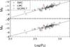 |
Fig. 12 Period-luminosity relation for RSGs. Diamond with vertical error bar: GCIRS 7. Squares and circles: SMC and LMC stars used in Yang & Jiang (2012). Line: best-fit law for the LMC+SMC (Yang & Jiang 2012, Table 5). |
The short primary period of RSGs follows a fairly tight period–luminosity (P–L) relation (Yang & Jiang 2012, and references therein). Figure 12 presents GCIRS 7 (MK = −11.3 ± 0.16, MH = −10.7 ± 0.2, P0 = 470 ± 10 d, see Table 1) on the P–L relationship for RSGs in the SMC and LMC. Given the uncertainty on the absolute magnitudes of GCIRS 7 and the intrinsic scatter around the best-fit relation, the agreement with the P–L relation is quite good, especially in the H band. The K-band magnitude of the star appears to be ≃0.1 mag too bright, which could be due to the circumstellar contribution discussed Sect. 4.1.
In contrast to the short primary period of RSGs, there is as of now no P–L relation established for the LSP. However, Kiss et al. (2006) have noticed a relation between the LSP, mass, and radius of RSGs. They considered W = P(M/M⊙)(R/R⊙)-2, which “is the natural form of the pulsation constant if the oscillations are confined to the upper layers of the envelope (Gough et al. 1965)”. They computed the average of W for 14 RSGs with P> 1000 d and found ⟨W⟩ = 0.082 ± 0.03. Taking P = 2620–2850 d, ⟨R⟩ = 1000 R⊙, and M = 22.5 M⊙ (Table 1, Sect. 4.1), we find W = 0.059–0.064 for GCIRS 7, within 1σ of the above mentioned average.
4.3. GCIRS 7 as an interferometric calibrator for GRAVITY
GCIRS 7 is the only star in the central parsec bright enough to be used as fringe-tracker reference with GRAVITY operating on the VLTI auxiliary telescopes (ATs). Furthermore, since this star is bright and close from the central black-hole candidate Sgr A*, it will be tempting to use it as a visibility calibrator whenever observing an object in the central parsec with GRAVITY, be it with the UTs or with the ATs.
However, GRAVITY will operate in the K band. The K-band visibilities of GCIRS 7 are affected by a significant, variable circumstellar contribution (Sect. 4.1). It will therefore be difficult to use this star as a visibility calibrator. Nevertheless, assuming the circumstellar geometry is simple enough (pending further investigations), one could perhaps use the star as a local calibration proxy. At any rate, the star must be considered interferometrically variable on the time scale of about one month, a fraction of the ≃470 d short period that we measured.
In addition, the size and nature of GCIRS 7 imply that convection cells may form in its atmosphere and affect the appearance of the photosphere (see e.g. Haubois et al. 2009; Freytag & Höfner 2008). Chiavassa et al. (2011) have shown that the photometric wobbling for a Betelgeuse-like star is of the order of 0.1 AU, corresponding to ≃10 μas at the distance of the Galactic centre. This is close to the expected astrometric accuracy of GRAVITY itself. This will limit the astrometric precision of studies of the nuclear star cluster using GCIRS 7 as astrometric reference. This limitation may be alleviated by systematically calibrating the astrometric zero point by observing one or several smaller or more stable stars.
4.4. Age of GCIRS 7 and the recent star burst
We list various physical parameters in Table 1, which are all consistent with each other. This gives good confidence in the age we derive for GCIRS 7: 6.5 to 10 Myr, depending on rotation. RSGs are in a rare state. The ratio of red to blue supergiants is approximately 0.4–0.5% (e.g. Pfuhl et al. 2011), so that there must be approximately 200 blue supergiants in the Galactic centre with the same age as GCIRS 7. There is a unique, well known population of >100 hot, massive stars in the central parsec, and the age we derive for GCIRS 7 is consistent the age estimated by several authors for this population (2–7 Myr, Genzel et al. 2003; 6 ± 2 Myr Paumard et al. 2006; Bartko et al. 2009). On the other hand, Lu et al. (2013) derived a 95% confidence interval for a cluster age of 2.5 to 5.8 Myr. This claim is not compatible with the age we derive for GCIRS 7.
Lu et al. (2013) relied essentially on the ratio of Wolf–Rayet (WR) to OB stars. This method has been recognised as strongly dependent on the prediction of evolutionary tracks (Schaerer & Vacca 1998). The evolution of a star beyond the main sequence, especially in the WR phase, is very sensitive to numerical and physical prescriptions, such as overshooting and mass loss rate. For an illustration, see e.g. Martins & Palacios (2013). In addition, the definition of a WR star does not rely on the same criteria in evolutionary models and in spectroscopic surveys. Finally, it is crucial to have a complete sample to correctly evaluate the observed ratio of WR to OB stars.
This is why in Paumard et al. (2006) we did not rely only on this indicator. In addition, we looked for the turn-off in the HR diagram (Paumard et al. 2006, Fig. 12), i.e. the position in the HR diagram of the most massive stars in the main sequence. The age of GCIRS 7 is now a third independent age indicator. Taken together, these indicators point towards a cluster age in the range 6–8 Myr. This age is actually permitted by the error bars in the right-hand panel of Fig. 3 of Lu et al. (2013), especially if one allows for a slightly flatter initial mass function than their preferred slope.
The simultaneous presence of both RSG and WR stars in a massive cluster presumably formed in a single burst of star formation is rare. For that to happen, the cluster must be young enough for the most massive stars to still be present (in the WR phase). At the same time, it must be old enough so that stars in the mass range 10–25 M⊙ have evolved to the RSG phase. That we are able to explain the presence of OB stars, WR stars, and the RSG GCIRS 7 using a single isochrone is a very strong indication that the central cluster is in this peculiar age range where all types of stars are present.
5. Conclusions
We have obtained interferometric fringes on GCIRS 7 with PIONIER on the six UT baselines of the VLTI at H-band. We were able to measure the photospheric size of the star: θUD(2013) ≃ 1.076 ± 0.093 mas translating to RUD(2013) ≃ 960 ± 92 R⊙ at R0 = 8.33 ± 0.35 kpc. K-band AMBER observations obtained in 2008 show a significant (≃20%) circumstellar excess and hint at photospheric and circumstellar variations. Photospheric temperature and size variations are confirmed by spectroscopy and photometry.
In addition, we reanalysed near infrared light curves of the star and found a prominent, long period of 2620–2850 days and a shorter period of 470 ± 10 days. The global peak-to peak variation has been ≃2 mag in the H band and ≃1.6 mag in the K band during the past 40 yr. The size we measured is quite consistent with the luminosity (⟨Mbol⟩ = −8.44 ± 0.22) and effective temperature (Teff = 3600 ± 195 K) of the star, and the short and long periods are in good agreement with the fundamental and long secondary period, respectively, for an RSG that size and that mass (22.5 ± 2.5 M⊙, Sect. 3.5). The physical parameters we derived are listed in Table 1.
Future observations of the Galactic centre nuclear star cluster may be performed with GRAVITY using GCIRS 7 as a fringe-tracker reference. Given the variable nature of this star and its environment, it may not be a stable phase reference at the expected accuracy of GRAVITY (10 μas) for durations of more than a few weeks. Therefore, it may be useful to calibrate the astrometric zero point on smaller or more stable stars regularly when using GCIRS 7 as a phase reference. Likewise, its usability as a (secondary) K-band visibility calibrator depends on whether the environment morphology is simple enough, pending further investigations.
Finally, the age we derive (6.5–10 Myr) is a confirmation of the cluster age (6 ± 2 Myr) we determined (Paumard et al. 2006; Bartko et al. 2009), and it contradicts recent claims for a younger cluster (2.5–5.8 Myr, Lu et al. 2013).
The calibrated data in the OI-FITS format (Pauls et al. 2005) will be included in the JMMC database http://www.jmmc.fr
Available at http://www.jmmc.fr/amberdrs
LITpro software available at http://www.jmmc.fr/litpro
Acknowledgments
We thank Myriam Benisty for help with the AMBER data reduction. This research made use of Jean-Marie Mariotti Centre products (the AMBER data reduction package3 and the LITpro4 service (Tallon-Bosc et al. 2008) co-developed by CRAL, LAOG, and FIZEAU), as well as of NASA’s Astrophysics Data System. We acknowledge financial support from the “Programme National de Physique Stellaire” (PNPS) of CNRS/INSU, France.
References
- Abuter, R., Schreiber, J., Eisenhauer, F., et al. 2006, New Astron. Rev., 50, 398 [NASA ADS] [CrossRef] [Google Scholar]
- Allen, C., & Cox, A. 2000, Allen’s astrophysical quantities (AIP Press) [Google Scholar]
- Arroyo-Torres, B., Wittkowski, M., Marcaide, J. M., & Hauschildt, P. H. 2013, A&A, 554, A76 [NASA ADS] [CrossRef] [EDP Sciences] [Google Scholar]
- Bartko, H., Martins, F., Fritz, T. K., et al. 2009, ApJ, 697, 1741 [NASA ADS] [CrossRef] [Google Scholar]
- Becklin, E. E., & Neugebauer, G. 1968, ApJ, 151, 145 [NASA ADS] [CrossRef] [Google Scholar]
- Becklin, E. E., & Neugebauer, G. 1975, ApJ, 200, L71 [NASA ADS] [CrossRef] [Google Scholar]
- Blum, R. D., Sellgren, K., & Depoy, D. L. 1996a, ApJ, 470, 864 [NASA ADS] [CrossRef] [Google Scholar]
- Blum, R. D., Sellgren, K., & Depoy, D. L. 1996b, AJ, 112, 1988 [NASA ADS] [CrossRef] [Google Scholar]
- Blum, R. D., Ramírez, S. V., Sellgren, K., & Olsen, K. 2003, ApJ, 597, 323 [NASA ADS] [CrossRef] [Google Scholar]
- Bonnet, H., Abuter, R., Baker, A., et al. 2004, The Messenger, 117, 17 [NASA ADS] [Google Scholar]
- Carr, J. S., Sellgren, K., & Balachandran, S. C. 2000, ApJ, 530, 307 [NASA ADS] [CrossRef] [Google Scholar]
- Chelli, A., Utrera, O. H., & Duvert, G. 2009, A&A, 502, 705 [NASA ADS] [CrossRef] [EDP Sciences] [Google Scholar]
- Chiavassa, A., Pasquato, E., Jorissen, A., et al. 2011, A&A, 528, A120 [NASA ADS] [CrossRef] [EDP Sciences] [Google Scholar]
- Claret, A. 2000, A&A, 363, 1081 [NASA ADS] [Google Scholar]
- Cunha, K., Sellgren, K., Smith, V. V., et al. 2007, ApJ, 669, 1011 [Google Scholar]
- Davies, B., Origlia, L., Kudritzki, R.-P., et al. 2009, ApJ, 694, 46 [NASA ADS] [CrossRef] [Google Scholar]
- Depoy, D. L., & Sharp, N. A. 1991, AJ, 101, 1324 [NASA ADS] [CrossRef] [Google Scholar]
- Eisenhauer, F., Abuter, R., Bickert, K., et al. 2003, in SPIE Conf. Ser. 4841, eds. M. Iye, & A. F. M. Moorwood, 1548 [Google Scholar]
- Eisenhauer, F., Perrin, G., Rabien, S., et al. 2008, in The Power of Optical/IR Interferometry: Recent Scientific Results and 2nd Generation, eds. A. Richichi, F. Delplancke, F. Paresce, & A. Chelli, 431 [Google Scholar]
- Ekström, S., Georgy, C., Eggenberger, P., et al. 2012, A&A, 537, A146 [NASA ADS] [CrossRef] [EDP Sciences] [Google Scholar]
- Freytag, B., & Höfner, S. 2008, A&A, 483, 571 [NASA ADS] [CrossRef] [EDP Sciences] [Google Scholar]
- Fritz, T. 2013, Ph.D. Thesis, Ludwig-Maximilians-Universitat, Munich [Google Scholar]
- Frogel, J. A., Stephens, A., Ramírez, S., & DePoy, D. L. 2001, AJ, 122, 1896 [NASA ADS] [CrossRef] [Google Scholar]
- Genzel, R., Schödel, R., Ott, T., et al. 2003, ApJ, 594, 812 [NASA ADS] [CrossRef] [PubMed] [Google Scholar]
- Genzel, R., Eisenhauer, F., & Gillessen, S. 2010, Rev. Mod. Phys., 82, 3121 [NASA ADS] [CrossRef] [Google Scholar]
- Gillessen, S., Eisenhauer, F., Trippe, S., et al. 2009, ApJ, 692, 1075 [NASA ADS] [CrossRef] [Google Scholar]
- Gough, D. O., Ostriker, J. P., & Stobie, R. S. 1965, ApJ, 142, 1649 [NASA ADS] [CrossRef] [Google Scholar]
- Haubois, X., Perrin, G., Lacour, S., et al. 2009, A&A, 508, 923 [NASA ADS] [CrossRef] [EDP Sciences] [Google Scholar]
- Kervella, P., Thévenin, F., Di Folco, E., & Ségransan, D. 2004, A&A, 426, 297 [NASA ADS] [CrossRef] [EDP Sciences] [Google Scholar]
- Kiss, L. L., Szabó, G. M., & Bedding, T. R. 2006, MNRAS, 372, 1721 [Google Scholar]
- Kleinmann, S. G., & Hall, D. N. B. 1986, ApJS, 62, 501 [NASA ADS] [CrossRef] [Google Scholar]
- Krabbe, A., Genzel, R., Eckart, A., et al. 1995, ApJ, 447, L95 [NASA ADS] [CrossRef] [Google Scholar]
- Le Bouquin, J.-B., Berger, J.-P., Lazareff, B., et al. 2011, A&A, 535, A67 [NASA ADS] [CrossRef] [EDP Sciences] [Google Scholar]
- Lenzen, R., Hartung, M., Brandner, W., et al. 2003, in SPIE Conf. Ser. 4841, eds. M. Iye, & A. F. M. Moorwood, 944 [Google Scholar]
- Levesque, E. M., Massey, P., Olsen, K. A. G., et al. 2005, ApJ, 628, 973 [NASA ADS] [CrossRef] [Google Scholar]
- Lomb, N. R. 1976, Ap&SS, 39, 447 [NASA ADS] [CrossRef] [Google Scholar]
- Lu, J. R., Do, T., Ghez, A. M., et al. 2013, ApJ, 764, 155 [NASA ADS] [CrossRef] [Google Scholar]
- Maness, H., Martins, F., Trippe, S., et al. 2007, ApJ, 669, 1024 [NASA ADS] [CrossRef] [Google Scholar]
- Martins, F., & Palacios, A. 2013, A&A, 560, A16 [NASA ADS] [CrossRef] [EDP Sciences] [Google Scholar]
- Nishiyama, S., Tamura, M., Hatano, H., et al. 2009, ApJ, 696, 1407 [NASA ADS] [CrossRef] [Google Scholar]
- Ott, T., Eckart, A., & Genzel, R. 1999, ApJ, 523, 248 [NASA ADS] [CrossRef] [Google Scholar]
- Pauls, T. A., Young, J. S., Cotton, W. D., & Monnier, J. D. 2005, PASP, 117, 1255 [NASA ADS] [CrossRef] [Google Scholar]
- Paumard, T., Genzel, R., Martins, F., et al. 2006, ApJ, 643, 1011 [NASA ADS] [CrossRef] [Google Scholar]
- Peeples, M. S., Stanek, K. Z., & Depoy, D. L. 2007, Acta Astron., 57, 173 [NASA ADS] [Google Scholar]
- Pfuhl, O., Fritz, T. K., Zilka, M., et al. 2011, ApJ, 741, 108 [NASA ADS] [CrossRef] [Google Scholar]
- Pott, J.-U., Eckart, A., Glindemann, A., et al. 2008, A&A, 487, 413 [NASA ADS] [CrossRef] [EDP Sciences] [Google Scholar]
- Rayner, J. T., Cushing, M. C., & Vacca, W. D. 2009, ApJS, 185, 289 [NASA ADS] [CrossRef] [Google Scholar]
- Rousset, G., Lacombe, F., Puget, P., et al. 2003, in SPIE Conf. Ser. 4839, eds. P. L. Wizinowich & D. Bonaccini, 140 [Google Scholar]
- Scargle, J. D. 1982, ApJ, 263, 835 [NASA ADS] [CrossRef] [Google Scholar]
- Schaerer, D., & Vacca, W. D. 1998, ApJ, 497, 618 [NASA ADS] [CrossRef] [Google Scholar]
- Schödel, R., Najarro, F., Muzic, K., & Eckart, A. 2010, A&A, 511, A18 [NASA ADS] [CrossRef] [EDP Sciences] [Google Scholar]
- Schreiber, J., Thatte, N., Eisenhauer, F., et al. 2004, in Astronomical Data Analysis Software and Systems (ADASS) XIII, eds. F. Ochsenbein, M. G. Allen, & D. Egret, ASP Conf. Ser., 314, 380 [Google Scholar]
- Serabyn, E., Lacy, J. H., & Achtermann, J. M. 1991, ApJ, 378, 557 [NASA ADS] [CrossRef] [Google Scholar]
- Tallon-Bosc, I., Tallon, M., Thiébaut, E., et al. 2008, in SPIE Conf. Ser., 7013 [Google Scholar]
- Tatulli, E., Millour, F., Chelli, A., et al. 2007, A&A, 464, 29 [NASA ADS] [CrossRef] [EDP Sciences] [Google Scholar]
- Tsvetkov, T. G. 1988, Ap&SS, 150, 223 [NASA ADS] [CrossRef] [Google Scholar]
- van Belle, G. T., Creech-Eakman, M. J., & Hart, A. 2009, MNRAS, 394, 1925 [NASA ADS] [CrossRef] [Google Scholar]
- Viehmann, T., Eckart, A., Schödel, R., et al. 2005, A&A, 433, 117 [NASA ADS] [CrossRef] [EDP Sciences] [Google Scholar]
- Yang, M., & Jiang, B. W. 2012, ApJ, 754, 35 [NASA ADS] [CrossRef] [Google Scholar]
- Yusef-Zadeh, F., & Morris, M. 1991, ApJ, 371, L59 [NASA ADS] [CrossRef] [Google Scholar]
- Zechmeister, M., & Kürster, M. 2009, A&A, 496, 577 [NASA ADS] [CrossRef] [EDP Sciences] [Google Scholar]
All Tables
Variations in Teff, MH, and RLD from the SINFONI spectra and NACO H-band photometry.
All Figures
|
Fig. 1 Projected baselines ((u,v) coverage) of the PIONIER (large symbols) and AMBER (small symbols) data. |
| In the text | |
|
Fig. 2 Example fringe waterfalls for one exposure. Each panel corresponds to one telescope pair. In each panel, the vertical axis corresponds to scan number (one scan lasts ≃1 s) and the horizontal axis to index within scan (which corresponds to optical path difference). In this specific example, fringes are present on all baselines. |
| In the text | |
|
Fig. 3 2013 H-band PIONIER data, V2 vs. spatial frequency in 106/rad or Mλ. Solid line: uniform-disk model of diameter 1.076 mas. Larger black symbols: first night, smaller grey symbols: second night. |
| In the text | |
|
Fig. 4 2008 K-band AMBER data, V2 vs. spatial frequency in 106/rad or Mλ. Lines: several two-component models where the star is represented by a uniform disk and the environment by: solid line: a circle, representing a thin shell; dashed line: a second uniform disk, representing a thick shell; dash-dotted line: a uniform background. |
| In the text | |
|
Fig. 5 J,H,Ks, and L-band light curves. The oldest data is from 1975, the latest from June 2013. Statistical uncertainties are represented, although they are often smaller than the symbol. Diamonds: NACO data; squares: from Peeples et al. (2007); circles: from Ott et al. (1999, these points have been brought up by 0.3 mag); triangles: from Blum et al. (1996a) which includes data from Becklin & Neugebauer (1975) and Depoy & Sharp (1991). Dashed curves: sinusoidal models with a period of 2850 d. |
| In the text | |
|
Fig. 6 SINFONI spectra. Only the three spectra with a resolution of ≃2000 are shown. Dark gray: MJD = 52 738; black: MJD = 55 383; light grey: MJD = 56 558. |
| In the text | |
|
Fig. 7 Top: H-band light curve after year 2000. Bottom: effective temperature measurements from SINFONI spectra. Diamonds: NACO data (fitted); squares: Peeples et al. (2007, for comparison). Dash-dotted, dark grey curve: best-fit two-period model. Dotted, light grey curve: second best-fit model. Vertical lines: dates of interferometric observations: March 2006 (Pott et al. 2008, K-band AMBER), May 2008 (K-band AMBER) and July 2013 (H-band PIONIER). Crosses: Teff from SINFONI spectra and the corresponding magnitude estimated using the best fit model; the vertical line of each cross indicates only the statistical uncertainty (see text, Sect. 3.3). |
| In the text | |
|
Fig. 8 Generalised Lomb-Scargle periodograms of the NACO light curves (bottom to top: H,K and L-band). Black curves: data periodograms. Light grey, dashed curve: single-period model. Dark grey, dash-dotted curve: two-period model. Vertical dotted lines: best fit periods. Vertical dashed lines: NACO time coverage in each band. The periodograms are normalised so that the expected power for pure Gaussian noise is 1. |
| In the text | |
|
Fig. 9 χ2 map for the two-period H-band model, normalised to its minimum of 4.68. The best-fit period pairs are marked by uncertainty crosses. |
| In the text | |
|
Fig. 10 CO-Teff calibration for RSGs with spectral types between G0 and M4. Open circles: stars from the IRTF library. The temperature uncertainty of the individual stars is 200 K (Allen & Cox 2000). Curve: best-fit empirical relation. Filled circles: EW(CO) measurements on GCIRS 7 and derived Teff. |
| In the text | |
|
Fig. 11 Position of GCIRS 7 in the H-R diagram (cross) compared with evolutionary tracks of stars with initial masses between Mini = 15 − 32 M⊙ with rotation (blue solid) and for Mini = 20 − 25 M⊙ without rotation (dashed green) from Ekström et al. (2012). The solid black lines denote the theoretical luminosities of stars with radii of R = 900,1100, and 1300 R⊙ as a function of effective temperature. |
| In the text | |
|
Fig. 12 Period-luminosity relation for RSGs. Diamond with vertical error bar: GCIRS 7. Squares and circles: SMC and LMC stars used in Yang & Jiang (2012). Line: best-fit law for the LMC+SMC (Yang & Jiang 2012, Table 5). |
| In the text | |
Current usage metrics show cumulative count of Article Views (full-text article views including HTML views, PDF and ePub downloads, according to the available data) and Abstracts Views on Vision4Press platform.
Data correspond to usage on the plateform after 2015. The current usage metrics is available 48-96 hours after online publication and is updated daily on week days.
Initial download of the metrics may take a while.